Direct Measurement of Effective Magnetic Diffusivity in Turbulent Flow of Liquid Sodium

Abstract

The first direct measurements of effective magnetic diffusivity in turbulent flow of electro-conductive fluids (the so-called $\beta$-effect) under magnetic Reynolds number ${\rm Rm}>>1$ are reported. The measurements are performed in a nonstationary turbulent flow of liquid sodium, generated in a closed toroidal channel. The peak level of the Reynolds number reached ${\rm Re}\approx 3\cdot 10^{6}$, which corresponds to the magnetic Reynolds number ${\rm Rm}\approx 30$. The magnetic diffusivity of the liquid metal was determined by measuring the phase shift between the induced and the applied magnetic fields. The maximal deviation of magnetic diffusivity from its basic (laminar) value reaches about $50\%$ .

Small-scale turbulence plays a crucial role in cosmic magnetism, providing the small-scale (turbulent) MHD-dynamo and contributing a lot to the dynamics of large-scale magnetic fields. The mean field (large-scale) dynamo equations are derived by applying the Reynolds approach to the magnetohydrodynamics (MHD) equations, and in the framework of the simplest case of homogeneous and isotropic (but mirror asymmetric) turbulence they can be reduced to Steenbeck et al. (1966)

$$\frac{\partial{\mathbf{B}}}{\partial t} = \nabla\times({\mathbf{U}}\times{\mathbf{B}})+\alpha\nabla\times{\mathbf{B}}+\eta\bigtriangleup{\mathbf{B}},$$

$$\nabla\cdot{\mathbf{B}} = 0,$$ (1)

where ${\mathbf{U}}$ and ${\mathbf{B}}$ describe the mean (large-scale) velocity and magnetic fields, $\eta=(\rho\mu)^{-1}+\beta$ is the magnetic diffusivity ($\rho$ - electrical resistivity, $\mu$ - magnetic permeability), and $\alpha$ and $\beta$ are the turbulent transport coefficients, describing the action of small-scale turbulent pulsations on the mean field dynamics (see e.g. Moffatt (1978); Krause and Rädler (1980)). Coefficient $\alpha$ describes the generation effects, and $\beta$ describes the contribution of turbulence to diffusion of the large-scale magnetic field. The knowledge of the magnetic turbulent transport coefficients $\alpha$ and $\beta$ is basic for astro- and geophysical applications in dynamo theory Zeldovich et al. (1983).

Over the last decade, major efforts were directed toward the study of MHD-dynamo in laboratory experiments (see for review Stefani et al. (2008)). The first-generation dynamo experiments are designed on the basis of strictly-specified large-scale flow. The Riga dynamo is driven by the cylindrical screw flow Gailitis et al. (2000), the Cadarache dynamo is based on a von Karman flow between two counterrotating disks Monchaux et al. (2007) and even the Karlsruhe dynamo, defined as a ”two-scale” dynamo, is driven by a set of strictly prescribed helical jets inside 52 tubes Stieglitz and Müller (2001). In this sense, all laboratory dynamos can be classified as quasi-laminar. In spite of that, the Reynolds numbers reached about $10^{7}$ and the flows were fully turbulent in all experiments. Thus, the role of turbulence is reduced in these experiments to enhancement of the diffusion of the magnetic field which, with a constant magnetic permeability, can be considered as an increase in effective resistance of liquid metal. The growth of resistivity can be crucial for dynamo experiments because of the corresponding reduction in magnetic Reynolds number. However, no direct measurement of effective resistivity in dynamo facilities has been performed up to now. An indirect indication of the beta-effect has been obtained in Madison sodium facilities by comparison of measured magnetic field and magnetic field simulated on the base of measured mean velocity field Spence et al. (2007). An interesting scheme of eddy diffusivity estimation from hydromagnetic Taylor-Couette flow experiment, recently suggested in Gellert and Rüdiger (2009).

The direct measurements of $\beta$ are impeded by the fact that the effect appears only under very large Reynolds numbers, when numerous side-effects prevent the accurate isolation of the $\beta$-effect. The first attempt of such measurements was done in a flow generated by a propeller in a vessel containing liquid sodium Reighard and Brown (2001), though the authenticity of the obtained data is questionable both with respect to the level of the observed conductivity variations and the estimates of the measurement errors.

A promising method of designing high Reynolds number flows (although nonstationary) in the limited mass of liquids was proposed in Frick et al. (2002), in which the flow was generated by the abrupt braking of a fast-rotating toroidal channel. Installation of diverters in the channel made it possible to create a toroidal screw flow of liquid gallium, in which, for the first time, was observed the $\alpha$-effect, defined by a joint action of the gradient of turbulent pulsations and large-scale vorticity Stepanov et al. (2006). The study of the dynamics of the nonstationary flow in a torus without diverters has shown that the development of the flow in the channel is attended by a strong short-time burst of turbulent pulsations with a peak in range on the order of $500-1000$Hz Noskov et al. (2009). This burst of small-scale turbulence provides an opportunity to detect the increase in effective resistivity of liquid metal using the low frequency alternating magnetic field ($\sim 100$ Hz). The idea of such an experiment has been realized in the nonstationary flow of liquid gallium. The toroidal channel made from textolite made it possible to get magnetic Reynolds number less than unity Denisov et al. (2008).

In this paper we exploit the similar experimental scheme using a titanium toroidal channel of larger size, filled with liquid sodium, which allowed us to increase the magnetic Reynolds number by two orders of magnitude.

The apparatus is an electro-mechanical construction mounted on a rigid frame, which is used as a support for a rotating toroidal channel (Fig. 1). The torus radius is $R=0.18$ m; the radius of the channel cross-section is $r=0.08$ m. The channel was filled with sodium in the vacuum and was placed into the air thermostat. The channel temperature may be stabilized in the range $(50-150)^{\circ}$C. The temperature sensor is mounted inside the channel and has good thermic contact with the sodium in both liquid and solid states.

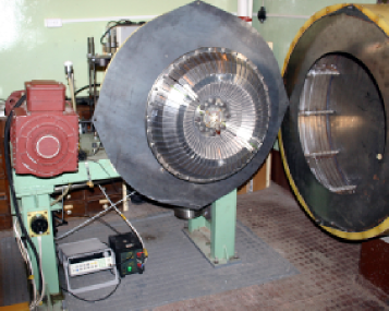
Figure 1: Titanium channel and thermostatic cover.

The channel is fastened on the horizontal axis, which is also used for mounting a driving pulley, a system of sliding contacts and a disk braking system. The frequency of the channel’s rotation is up to 45 r.p.s. and the flow in the channel is generated by abrupt braking – the braking time is no more than $0.3$ sec. The maximum velocity of the flow is reached after channel is stopped and achieves about $70$ % of the linear velocity of the channel before braking. This means that the Reynolds number ${\rm Re}=Ur/\nu$ ($\nu$ is the kinematic viscosity of the liquid sodium) reaches at maximum the value ${\rm Re}\approx 3\cdot 10^{6}$, which corresponds to the magnetic Reynolds number ${\rm Rm}=Ur\rho\mu\approx 30$.

The data-gathering system is based on an NI Data Acquisition System and is a part of an electrical measuring system, whose schematic circuit is shown in Fig. 2. The ’Generator/Amplifier’ block creates in the toroidal coil a stabilized sinusoidal current with frequency $30<\nu<1000$ Hz, which produces an alternating toroidal magnetic field inside the channel. Besides the toroidal coil, two diametrically located magnetic-test coils are wound around the channel.

Figure 2: Schematic circuit of the measuring system. $U_{dp}$, $U_{T}$, $E$ and $U$ are the driving pulse, the tachometer signal, the electromotive force of magnetic-test coil and the voltage, corresponding to applied current.

The change in phase shift $\theta$ between the measured magnetic field and the alternating current in the toroidal coil is a value, which can be treated as a measure of logarithmic changes of diffusivity of the sodium

$$\Delta\theta\backsimeq C\frac{\Delta\rho}{\rho}=C\frac{\Delta\eta}{\eta},$$ (2)

where $C$ is a dimensional coefficient, which depends on the geometry and resistivity of the channel wall, and on the frequency of the applied magnetic field. The measuring system is completed with software, based on wavelet analysis, which provides calculation of the time dependence of phase shift after signals recording. Wavelets are required because the variation of phase shift occurs at times comparable with the oscillation period.

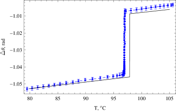
Figure 3: Phase shift versus sodium temperature in the channel at frequency $\nu=97$ Hz: experiment (points) and simulations (solid line).

The measurement system has been tested and calibrated by measuring the dependence of the sodium resistivity on the temperature. The channel containing the sodium was cooled down from $105^{\circ}$C to $80^{\circ}$C. This range of temperature includes the sodium freezing point, which gives the best measure for calibration because the resistivity of the sodium decreased at that point by $31$% percent, while the temperature remained constant. This excludes the influence of resistivity variation of titanium, coils, etc. Fig. 3 shows the results of phase shift measurements performed at frequency $\nu=97$ Hz, together with results of numerical simulations. For this frequency, the skin layer thickness of titanium is about $44$ mm (the mean thickness of titanium wall is about $10$ mm) and the skin layer thickness of sodium is about $16$ mm.

Theoretical phase shift in the skin layer of an infinite cylindrical solenoid, which includes a titanium cylinder tube with sodium, fits the experimental points well, and allows us to define the factor of proportionality in relation (2) for each applied frequency. For the case $\nu=97$Hz, shown in Fig. 3, $C=102\pm 3$ mrad. For verification of the method, an alternative approach of evaluating the sodium resistivity was used, based on the equivalent electrotechnical schematic of the transformer with the short-circuited secondary winding, which gave close results.

All dynamical experiments concerning the turbulent flow of liquid sodium were performed under the fixed temperature $T=(102\pm 1)^{\circ}$C. The estimation of sodium heating due to energy dissipation in decaying turbulent flow at the highest rotational velocity $f=50$ r.p.s. (considering that its entire kinetic energy will dissipate in the heat) gives $\Delta T\approx 0,8^{\circ}$C, which corresponds to variations of resistivity less than $0.5$%.

Results and Summary. The rotational velocity $\Omega$ varied from $10$ to $45$ r.p.s. with a step of $5$ r.p.s. Measurements for all $\Omega$ were performed using three different frequencies $\nu$ ($53$, $66$ and $97$ Hz). The evolution of the phase shift, measured at frequency $\nu=97$ Hz for different velocity of channel rotation $\Omega$, is shown in Fig. 4. Each curve is the result of averaging over 10 realizations. The end of braking is defined as the reference time point ($t=0$). One can see that braking generates the turbulent flow, the maximal intensity of which coincides with the end of braking. At this moment the phase shift also reaches its maximum. Later on, turbulent pulsations rapidly decay and the phase shift reduces to zero.

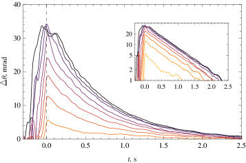
Figure 4: Phase shift variations with flow evolution for channel rotation rate $\Omega=10,15,...,40,45$ r.p.s. (bottom-up) in linear and lin-log (inset) scales. $\nu=97$ Hz.

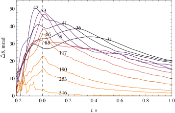
Figure 5: Phase shift variations with flow evolution for channel rotation rate $\Omega=40$ r.p.s. and different frequency $\nu$, shown near each curve.

The inset of Fig. 4 shows that the measured phase shift decays exponentially, which contradicts the ideas about the free decay of developed turbulence, which are rested on the power laws. The turbulent boundary layer in the nonstationary toroidal flow is developed in a very specific way. This was found in studies of the dynamics of a similar flow of liquid gallium, which have shown that the decay of the mean energy of the turbulent flow in the toroidal channel follows the $t^{-2}$ law, while the burst of turbulent pulsations attends the flow formation and deceases abruptly Noskov et al. (2009). This is an additional argument to suppose that the measured phase shift is mostly caused by small-scale turbulence, but not by the dynamics of the mean flow.

We have examined the flow across a broad range of frequencies, $31\leq\nu\leq 516$ Hz (the skin layer thickness varies then from $29$ to $7$ mm). Fig. 5 shows the phase shift evolution for different frequencies and it confirms the general idea that the turbulent diffusivity should follow the intensity of turbulent pulsation, which grows from the wall of the channel to its center – at a low frequency the contribution of the central part of the flow is larger and the $\beta$-effect is more pronounced. At its highest frequency the measuring system senses only the boundary layer, which developed first: for $\nu=516$ Hz the phase shift achieves the maximum at $t=-0.15$ sec, while for $\nu=31$ Hz the maximum appears only at $t=0.4$ sec.

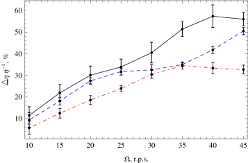
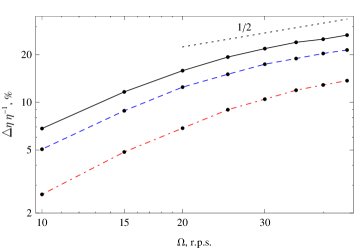
Figure 6: Relative increase of magnetic diffusivity (percentage) versus channel rotation rate $\Omega$ at the end of braking (top) and at $0.7$ sec later (bottom): $\nu=53$ Hz (solid, black), $\nu=66$ Hz (dashed, blue), $\nu=97$ Hz (dash-dot, red). The lower panel is shown in logarithmic scale; dots show the power law ”1/2”.

In Fig. 6 we show how the observed $\beta$-effect depends on the intensity of the mean flow (on the Reynolds number, which is defined by the channel rotation rate before braking). First, we show (in the upper panel) the maximal deviation of effective magnetic diffusivity, which corresponds to the end of braking, from the basic value. Measurements are taken using three frequencies: $\nu=53$, $66$, and $97$ Hz. Changing frequency, we vary the depth of penetration of magnetic field into the turbulent flow. As the frequency is lowered, the thicker the skin layer becomes and the more pronounced is the observed $\beta$-effect. The maximal value (for $\Omega=45$ r.p.s. and $\nu=53$ Hz) exceeds $50$%. At low rotation rates the effect increases monotonically, in a similar manner for all frequencies; however, with $\Omega>30$ r.p.s., the monotony is disrupted and the curves develop in disorder. Examining individual curves for different realizations, it is possible to see that with high rotational speeds, the structure of the curve near the maximum becomes very complex – the maximum becomes wider with a kind of plateau, against the background which appears to be separate distinct maximums. All these peculiarities disappear very shortly – in Fig. 4 one can see that at $t\approx 0.2-0.3$, all curves evolve quite similar without any deviation. We show in the lower panel of Fig. 6 the deviation of effective magnetic diffusivity at $t=0.7$ sec. Then all three curves show similar monotonic increase of the $\beta$-effect. Shown in logarithmic scales, they display a tendency toward a power law $\Delta\eta\sim\Omega^{1/2}$ at high rotational velocity.

So, the measurement of electric conductivity in the nonstationary fully developed turbulent (${\rm Re}\lesssim 3\cdot 10^{6}$) flow of liquid sodium in a closed channel shows that the effective magnetic diffusivity essentially increases with the Reynolds number. For the maximal rotation rate $\Omega=45$ r.p.s., which corresponds to ${\rm Rm}\approx 30$, the maximal deviation of magnetic diffusivity reaches about $50$%. Experiments with liquid gallium at low magnetic Reynolds number (${\rm Rm}<1$) revealed a quadratic like dependence $\beta\sim({\rm Rm})^{2}$ Denisov et al. (2008), which corresponds to general conceptions of the beta-effect for low ${\rm Rm}$. Our results show that the quadratic law does not hold at moderate ${\rm Rm}$. Note that the turbulent viscosity in stationary pipe flows at high $\rm Re$ increases as $\nu_{t}\sim{\rm Re}^{1/2}$ Schlihting (1964) and our results show at the highest Reynolds numbers a tendency to the same power law. One should treat the obtained dependence to the case of stationary pipe flow, or to homogeneous turbulence, with great caution. However, in view of the fact that the problem of measuring the examined characteristic in real flows is very complicated, and that experimental data are completely absent, measurement of the effective magnetic diffusivity in the turbulent medium, even in one particular case, is an important step toward the experimental substantiation of general MHD-dynamo conceptions.

This work was supported by ISTC project 3726 and RFBR-SNRS grant No. 07-01-92160.

References

- Steenbeck et al. (1966) M. Steenbeck, F. Krause, and K. Rädler, Z. Naturforsch. A 21, 369 (1966).
- Moffatt (1978) H. K. Moffatt, Magnetic Field Generation in Electrically Conducting Fluids (Cambridge University Press, Cambridge, 1978).
- Krause and Rädler (1980) F. Krause and K.-H. Rädler, Mean-field Magnetohydrodynamics and Dynamo Theory (Pergamon Press, New York, 1980).
- Zeldovich et al. (1983) Y. B. Zeldovich, A. A. Ruzmaikin, and D. D. Sokoloff, Magnetic Fields in Astrophysics (New York: Gordon and Breach, 1983).
- Stefani et al. (2008) F. Stefani, A. Gailitis, and G. Gerbeth, Zamm-Zeitschrift Fur Angewandte Mathematik Und Mechanik 88, 930 (2008).
- Gailitis et al. (2000) A. Gailitis, O. Lielausis, S. Dement’ev, E. Platacis, A. Cifersons, G. Gerbeth, T. Gundrum, F. Stefani, M. Christen, H. Hänel, et al., Phys. Rev. Lett. 84, 4365 (2000).
- Monchaux et al. (2007) R. Monchaux, M. Berhanu, M. Bourgoin, M. Moulin, P. Odier, J. Pinton, R. Volk, S. Fauve, N. Mordant, F. Pétrélis, et al., Phys. Rev. Lett. 98, 044502 (2007).
- Stieglitz and Müller (2001) R. Stieglitz and U. Müller, Phys. Fluids 13, 561 (2001).
- Spence et al. (2007) E. J. Spence, M. D. Nornberg, C. M. Jacobson, C. A. Parada, N. Z. Taylor, R. D. Kendrick, and C. B. Forest, Phys. Rev. Lett. 98, 164503 (2007).
- Gellert and Rüdiger (2009) M. Gellert and G. Rüdiger, Phys. Rev. E 80, 046314 (2009).
- Reighard and Brown (2001) A. B. Reighard and M. R. Brown, Phys. Rev. Lett. 86, 2794 (2001).
- Frick et al. (2002) P. Frick, V. Noskov, S. Denisov, S. Khripchenko, D. Sokoloff, R. Stepanov, and A. Sukhanovsky, Magnetohydrodynamics 38, 143 (2002).
- Stepanov et al. (2006) R. Stepanov, R. Volk, S. Denisov, P. Frick, V. Noskov, and J. Pinton, Phys. Rev. E 73, 046310 (2006).
- Noskov et al. (2009) V. Noskov, R. Stepanov, S. Denisov, P. Frick, G. Verhille, N. Plihon, and J. Pinton, Phys. Fluids 21, 045108 (2009).
- Denisov et al. (2008) S. A. Denisov, V. I. Noskov, R. A. Stepanov, and P. G. Frick, JETP Lett. 88, 167 (2008).
- Schlihting (1964) H. Schlihting, Grenzschicht-Theories (G.Braun, Karlsruhe, 1964).