Strong Correlations in Actinide Redox Reactions

Abstract

Reduction-oxidation (redox) reactions of the redox couples An(VI)/An(V), An(V)/An(IV), and An(IV)/An(III), where An is an element in the family of early actinides (U, Np, and Pu), as well as Am(VI)/Am(V) and Am(V)/Am(III), are modeled by combining density functional theory with a generalized Anderson impurity model that accounts for the strong correlations between the 5f electrons. Diagonalization of the Anderson impurity model yields improved estimates for the redox potentials and the propensity of the actinide complexes to disproportionate.

I Introduction

Chemical reactions of the early actinide elements in aqueous solution are complex and challenging to predict. Elements U, Np, and Pu each have four or more oxidation states in acidic environments (Am has three). Two of these states (III and IV) are hydrated An³⁺ and An⁴⁺ ions; the other two (V and VI) form linear trans-dioxo AnO${}_{2}^{+}$ and AnO${}_{2}^{2+}$ actinyl complexes. Disproportionation reactions are common, especially in the case of plutonium for which three of the redox potentials are nearly the same (about one volt). As different oxidation states have widely different solubilitiesFanghanel:2002 , redox chemistry plays a crucial role in the environmental dispersal of actinides.Choppin:2001 The rich behavior of actinide ions may be traced to the valence electrons, especially those in the 5f shell.Clark:2000 Because the 5f orbitals are relatively localized, the Coulomb interaction induces strong correlations between electrons in the shell. The possibility that strong correlations in these solvated actinide and actinyl ions enhance tendencies to disproportionate is an intriguing hypothesis. Support for this idea is provided by a Hubbard model of 5f electrons that disproportionates when solved in the Hartree-Fock (HF) approximation.Runge:2004p334

Quantitative models of actinide reactions must overcome several obstacles.Schreckenbach:2010p126 First relativity and the energetics of solvation must be taken into account. At present only the density functional theory (DFT) method is capable of modeling these aspects accurately. However, incorporating the physics of strong electronic correlations among the 5f electrons presents a greater challenge as these are known to be poorly captured by DFT.Roberto:2006p44 In this paper we take a hybrid approach to solving these problems by using DFT to construct a generalized Anderson impurity model of the frontier orbitals.Straus:1995p464 ; Hubsch:2006 ; Labute:2002 ; Labute:2004 ; Marston:1993p450 ; Onufriev:1996p451 Exact diagonalization of the Anderson impurity model corrects the free energy obtained from DFT alone, yielding improved predictions for redox free energies. We emphasize that the hybrid method outlined here differs markedly from the LDA+U approach as it does not simply modify the LDA functional to partly account for the Coulomb repulsion; rather a high-dimensional many-electron Hamiltonian that models the physics of strong correlations between the important low-energy states is diagonalized. The approach also differs from configuration-interaction (CI) and its variantsBartlett:2007p315 in two significant ways: First we are able to exactly diagonalize the low-energy effective model with no restrictions placed on the ground state wavefunction. Second, the two-body Coulomb interaction is not the bare electron-electron repulsion but rather an effective interaction that takes into account the effects of screening.

The rest of the paper proceeds as follows: In Sec. II we discuss the ab initio part of the calculation and compare the results we obtain to calculations by other workers. The independent-particle model that describes the Kohn-Sham (KS) orbitals and the spin-orbit interaction is introduced in Sec. III. Incorporation of the effective Coulomb interaction via a many-body model of the low-energy degrees of freedom is carried out in Sec. IV. The physics of strong correlations are illustrated with the use of a simplified model in Sec. V. The calculation of redox potentials and other observables by the hybrid approach are presented in Sec. VI. We conclude with some discussion in Sec. VII.

II Density Functional Theory

DFT based studies of early actinides in aqueous solution have modeled the structure, vibrational frequencies, and free energies of hydration.Schreckenbach:1998 ; Spencer:1999 ; Blaudeau:1999p463 ; Hay:2000 ; Tsushima:2001 ; Vallet:2001a ; Vallet:2004p370 ; Tsushima:2005 ; Sonnenberg:2005 ; Cao:2005 ; Shamov:2005 ; Gutowski:2006 We do not attempt to review this work comprehensively here but refer the reader instead to Ref. Schreckenbach:2010p126, and references therein. As there is significant hybridization between the higher orbitals, accurate calculations require full quantum mechanical treatment of all orbitals with principal quantum number $n=5$ and higher.Kuchle:1994 ; Odoh:2010p124 Using small cores, ab initio calculations performed by Shamov and SchreckenbachShamov:2005 were able to reproduce An(VI)/An(V) redox potentials to within $0.6$ volt of the measured values.

The Amsterdam Density Functional (ADF)ADF is an attractive DFT package for modeling actinides in solution because it includes relativistic corrections via the zeroth-order regular approximation (ZORA)van-Lenthe:1993 ; van-Lenthe:1996b , uses a basis of localized Slater-type atomic orbitals, and models solvation with the Conductor like Screening Model (COSMO).Klamt:1995 In our calculations the first coordination sphere of water molecules are treated quantum mechanically; COSMO is used to simulate a bulk dielectric medium beyond the sphere. Quantum mechanical modeling of the second sphere of hydration may lead to improved agreement with experimentGutowski:2006 but we defer that for future work. For the sake of simplicity the number of water molecules in the first solvation sphere are kept constant for each oxidation state: Eight each in the case of An(III) and (IV) and five for AnO₂(V) and (VI). (As discussed later, we find that coordinating Pu(III) with 9 water molecules makes only a small difference.) We use the revised PBE exchange-correlation functional.Hammer:1999 ; Perdew:1996 ; Vosko:1980 For the actinides we employ a basis set modified from ADF’s triple-$\zeta$, doubly polarized (TZ2P) ZORA wavefunctions. The frozen core consists of the 60 orbitals for which $n\leq 4$. The ADF-supplied basis set has 78 frozen core orbitals; 60 of these are retained in the core and the 5s, 5p, and 5d orbitals are promoted to valence orbitals. The number of sets of fit functions is accordingly increased from 79 to 87. For oxygen and hydrogen the relativistic TZ2P all-electron basis set provided by ADF is employed with no modification.

Spin-unrestricted calculations are carried out in three stages. As a first step the geometry of the actinide (or actinyl) plus the first solvation sphere is optimized in the gas-phase (no COSMO). We verify that all vibrational modes have real frequencies at the optimal geometry; these frequencies are used later in the thermodynamic calculations. The geometry is then allowed to relax in solvation within the COSMO approximation for the surrounding dielectric, with the following cavity radii: 1.350 Å  (H), 1.517 Å  (O) and 2.10 Å  (An). Thermodynamic properties are calculated in the ideal gas approximation with an effective pressure of 1354 atmospheres to account for the reduced entropy of translation as appropriate for the aqueous environment.Martin:1998 As a final step an independent-particle model of the frontier orbitals is constructed (see Sec. III) and the single-electron spin-orbit interaction is added to correct the electronic contribution to the free energy.

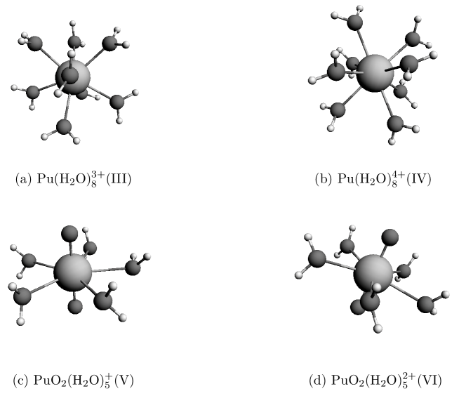
Figure 1: Converged geometries of the plutonium complexes.

Minimum energy configurations are found to have highly symmetrical geometries consistent with X-ray absorption fine structure (XAFS) and extended-XAFS (EXAFS) measurements. For example, the geometry of the Pu(III) and Pu(IV) complexes converge to the cubic configuration shown in Fig. 1 while the actinyls form pentagonal bipyramids. Interestingly, the converged geometry of the Pu(V) actinyl complex (Fig. 1 (c)) rotates one of the water molecules so that both hydrogen atoms are on the same side of the molecular equatorial plane. This distortion of the molecular symmetry is also seen in the converged geometries of U(VI), Np(VI), Pu(V), Am(V) and Am(VI). Table 1 shows the calculated bond lengths of the four oxidation states. The calculated geometries compare well with those found in previous DFT studiesCao:2005 ; Hay:2000 ; Shamov:2005 ; Sonnenberg:2005 ; Tsushima:2001 ; Tsushima:2005 of actinyls in solution and also, as shown in Fig. 2, with available experimental measurements, though DFT overestimates the mean An-OH₂ bond lengths by up to 0.1 Å  in the case of the actinyls.

Table 1: Calculated and selected experimental internuclear distances (Å). The calculated lengths are means over all bonds of the given type.

		V				VI
		U	Np	Pu	Am	U	Np	Pu	Am
An=O${}_{\text{eq}}$	Calc.	1.84	1.81	1.80	1.80	1.79	1.76	1.74	1.74
	Exp.		1.81	1.81		1.76	1.75	1.74
			1.85			1.78
						1.702
An-OH2	Calc.	2.61	2.60	2.62	2.65	2.49	2.47	2.47	2.50
	Exp.		2.47	2.47		2.41	2.42	2.40
			2.50			2.421
		III				IV
		U	Np	Pu	Am	U	Np	Pu
An-OH2	Calc.	2.53	2.52	2.50	2.50	2.40	2.38	2.38
	Exp.	2.61	2.52	2.49	2.48	2.41	2.39	2.39
			2.51			2.40

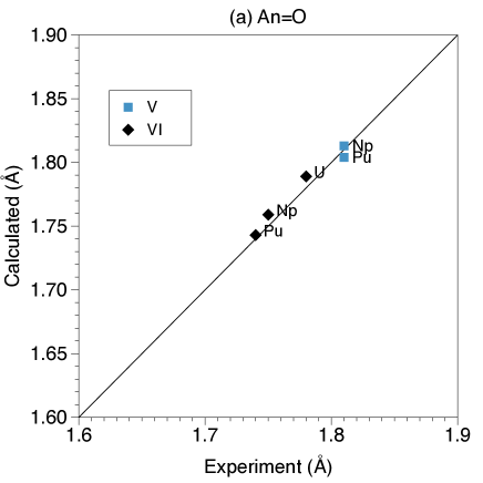
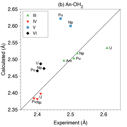
Figure 2: Selected calculated mean internuclear distances compared to experimental values for (a) An=O actinyl bonds and (b) An-OH₂ bonds between the actinide atom and water molecules in the first solvation sphere.

Figure 3: Reduction potentials (volts) as calculated by DFT and corrected for the spin-orbit interaction compared to measured values as detailed in Ref. Bratsch:1989, ; see however Ref. Kihara:1999p333, for a different compilation of measured redox potentials with slightly different values. PBE and B3LYP DFT results, corrected for spin-orbit and multiplet interactions, are from Table 10 of Ref. Shamov:2005, .

To calculate the redox potentials we follow the procedure outlined in Refs. Hay:2000, and Shamov:2005, , extending that work to include the An(V)/An(IV) and An(IV)/An(III) redox couples as well as reactions involving americium. The three half-reactions are as follows:

$$\text{AnO}_{2}\text{(H}_{2}\text{O)}_{5}^{2+}(\text{VI})+\text{e}^{-} \rightarrow \text{AnO}_{2}\text{(H}_{2}\text{O)}_{5}^{+}(\text{V})$$

$$\text{AnO}_{2}\text{(H}_{2}\text{O)}_{5}^{+}(\text{V})+4\text{H}_{3}\text{O}^{+}+\text{e}^{-} \rightarrow \text{An}\text{(H}_{2}\text{O)}_{8}^{4+}(\text{IV})+3\text{H}_{2}\text{O}$$

$$\text{An}\text{(H}_{2}\text{O)}_{8}^{4+}(\text{IV})+\text{e}^{-} \rightarrow \text{An}\text{(H}_{2}\text{O)}_{8}^{3+}(\text{III})\ .$$ (1)

Potentials are obtained from the free energies of the following three full reactions:

$$\text{AnO}_{2}\text{(H}_{2}\text{O)}_{5}^{2+}(\text{VI})+\frac{1}{2}\text{H}_{2}(g)+\text{H}_{2}\text{O} \rightarrow \text{AnO}_{2}\text{(H}_{2}\text{O)}_{5}^{+}(\text{V})+\text{H}_{3}\text{O}^{+}$$

$$\text{AnO}_{2}\text{(H}_{2}\text{O)}_{5}^{+}(\text{V})+3\text{H}_{3}\text{O}^{+}+\frac{1}{2}\text{H}_{2}(g) \rightarrow \text{An}\text{(H}_{2}\text{O)}_{8}^{4+}(\text{IV})+2\text{H}_{2}\text{O}$$

$$\text{An}\text{(H}_{2}\text{O)}_{8}^{4+}(\text{IV})+\frac{1}{2}\text{H}_{2}(g)+\text{H}_{2}\text{O} \rightarrow \text{An}\text{(H}_{2}\text{O)}_{8}^{3+}(\text{III})+\text{H}_{3}\text{O}^{+}\$$ (2)

using the zero-potential reference half-reaction of the standard hydrogen electrode (SHE) $\text{H}^{+}+\text{e}^{-}\rightarrow\frac{1}{2}\text{H}_{2}(\text{g})$. We note that the free energy of the hydronium reaction $\text{H}_{3}\text{O}^{+}\rightarrow\text{H}^{+}+\text{H}_{2}\text{O}$ as calculated within DFT is $-5.33$ eV.

Because Am(IV) is unstable, in the case of americium the V/III redox potential is calculated in lieu the V/IV and IV/III redox couples. In this case, the reduction half reaction is:

$$\text{AmO}_{2}\text{(H}_{2}\text{O)}_{5}^{+}(\text{V})+4\text{H}_{3}\text{O}^{+}+2\text{e}^{-} \rightarrow \text{Am}\text{(H}_{2}\text{O)}_{8}^{3+}(\text{III})+3\text{H}_{2}\text{O}$$ (3)

corresponding to the full reaction

$$\text{AmO}_{2}\text{(H}_{2}\text{O)}_{5}^{+}(\text{V})+2\text{H}_{3}\text{O}^{+}+\text{H}_{2}(g) \rightarrow \text{Am}\text{(H}_{2}\text{O)}_{8}^{3+}(\text{III})+\text{H}_{2}\text{O}\ .$$ (4)

Fig. 3 compares the calculated potentials to experiment; the calculated potentials include the contribution from the one-particle spin-orbit interaction as described below in Sec. III. The VI/V potentials for U, Np, and Pu are qualitatively consistent with previous work despite differences in the DFT packages. We find redox potentials, including the spin-orbit interaction, of respectively $-0.44$, $0.31$ and $0.94$ volts. These compare to values $2.37$, $4.00$ and $3.28$ volts found by Hay, Martin, and SchreckenbachHay:2000 who used Gaussian 98, relativistic core potentials, and the hybrid B3LYP functional, and included multiplet interactions corrections. However, Shamov and SchreckenbachShamov:2005 ; Shamov:2006p12072 following a similar procedure but with a smaller ($n\leq 4$ frozen core obtained $-0.10$, $1.72$ and $1.29$ volts in better agreement with experiment ($0.160$, $1.236$ and $0.966$ volts)Bratsch:1989 , highlighting the importance of treating all orbitals with $n>4$ dynamically. Use of the Priroda PBE functional yielded comparable redox potentials of $-0.51$, $0.87$ and $0.43$ volts.Shamov:2005 When the multiplet interaction correction is removed these VI/V potentials they show the same trend as our calculated DFT potentials , increasing monotonically from U to Np to Pu.

As mentioned above we only study the case of first solvation spheres of An(III) and An(IV) with 8 water molecules. Ref. Clark:2006p427, reports alternative molecular geometries for plutonium ions, with Pu(III) surrounded instead by 9 coordinating water molecules (see also Refs. Blaudeau:1999p463, and Tsushima:2005, ). A DFT calculation of the free energy of Pu(III) with nine water molecules finds it to be lower by $0.09$ eV, a small change in comparison to the other corrections that we consider here.

III Independent Particle Model

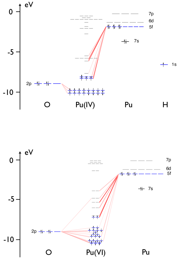
Figure 4: KS molecular orbital energy levels and their atomic fragment composition for the Pu(IV) (top) and Pu(VI) (bottom) complexes, highlighting the importance of the 5f and axial (actinyl) 2p orbitals near the HOMO/LUMO boundary. The relative size of the contributions from the Löwdin atomic orbitals is indicated by the thickness of the lines. (Hydrogen orbitals are not shown for Pu(VI) and O includes contributions from both the actinyl ligands and the water molecules.) As indicated the atomic fragments have equal numbers of up and down electrons, but the complex has greater numbers of up electrons, as the spin-unrestricted DFT calculations satisfy Hund’s rule.

We turn next to the construction of the independent-particle model of the frontier orbitals that includes the spin-orbit interaction and serves as the starting point for the many-body Anderson impurity model:

$$\hat{H}_{indep}=\hat{H}_{ks}+\hat{H}_{so}\ .$$ (5)

We make the usual assumption that KS fermions may be regarded as physical electrons, when in fact the connection between the two is subtle: The DFT ground state is a Slater determinant of KS fermions whereas the electron wavefunction is not generally described by a single determinant. Conveniently ADF expresses the KS eigenstates as linear combinations of localized orbitals orthonormalized by the Löwdin procedureLowdin:1950 . These Slater-type orbitals, expressed in terms of Cartesian spherical harmonics, form the basis that we work in. In this way the KS orbitals are projected onto the Hilbert subspace that retains only the actinide 5f Löwdin orbitals and, in the case of the actinyls, 2p Löwdin orbitals on the two oxygen ligands. As Fig. 4 shows, these are the atomic orbitals that are the most important constituents of the KS orbitals near the HOMO/LUMO boundary. For the actinyls, $14+6+6=26$ Löwdin orbitals are thus retained; for oxidation states III and IV only the 14 5f orbitals are required. Although it would be desirable to also retain the An 6d Löwdin orbitals which are close in energy to the An 5f orbitals, and also the Löwdin orbitals in the first solvation sphere of water molecules, the resulting many-body Hilbert space would be too large for exact diagonalizations to be carried out.

In the case of the actinyls the resulting effective Hamiltonian of the frontier orbitals may be written:

$$\hat{H}_{ks}=\sum_{ij\sigma}\epsilon^{f}_{ij\sigma}f^{\dagger}_{i\sigma}f_{j\sigma}+\sum_{ab\sigma}\epsilon^{p}_{ab\sigma}p^{\dagger}_{a\sigma}p_{b\sigma}+\sum_{ia\sigma}(t_{ia\sigma}f^{\dagger}_{i\sigma}p_{a\sigma}+H.c.)\ .$$ (6)

Operator $f^{\dagger}_{i\sigma}$ ($p^{\dagger}_{a\sigma}$) creates an electron in the 5f (2p) Löwdin orbital with spin $\sigma$ and spatial state $i$ ($a$) in the Cartesian spherical harmonic basis. In Eq. 6 $\epsilon^{f}_{ij\sigma}$ and $\epsilon^{p}_{ab\sigma}$ are matrix elements for, respectively, the An 5f and O 2p Löwdin orbitals, and $t_{ia\sigma}$ are the hopping amplitudes between the 5f and 2p orbitals. Oxidation states III are IV are modeled by the first term in Eq. 6 alone. Parameters $\epsilon$ and $t$ are obtained by calculating the matrix elements of the KS Hamiltonian, which is diagonal in the basis of KS orbitals, in the basis of the 5f (and in the case of actinyls, 2p) Löwdin orbitals. The matrix elements may then be grouped into the amplitudes that appear in Eq. 6.

Figure 5: Comparison of the KS molecular orbital energies against those of the independent-particle model that describes the projected 5f and 5f-2p subspaces, for the cases of U(III) and U(V). Shading of the KS orbitals indicate the relative size of their contribution to the 5f or 5f-2p Löwdin subspace, with the lightest lines representing orbitals that make little or no contribution.

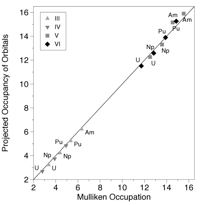
Figure 6: Total electronic occupation of the An 5f and (in the case of actinyls) O 2p Löwdin orbitals as calculated by projection of the occupied KS molecular orbitals onto the Löwdin atomic orbitals, compared to that found by Mulliken analysis.

The truncation of the full Hilbert space to the subspace consisting only of An 5f and (actinyl) O 2p Löwdin orbitals introduces error into the calculations. Fig. 5 shows how the single-particle energies of the projected independent-particle model match those of the full unprojected KS levels for the cases of U(III) and U(V). In Fig. 6 the total electronic occupation of the An 5f and (actinyl) O 2p Löwdin orbitals as calculated by projection of the occupied KS molecular orbitals onto the Löwdin atomic orbitals is compared to the corresponding occupancies found by Mulliken analysis. The occupancy of oxidation states III and IV agree to within 2% of that found by Mulliken analysis; and to within 4% for oxidation states V and VI.

As it stands Eq. 5 has no spin-flip processes, reflecting the limitation of DFT which is formulated in terms of separate densities of spin-up and down electrons. The one-electron spin-orbit interaction for the 5f Löwdin orbitals, $\hat{H}_{so}=\zeta\vec{\ell}\cdot\vec{s}+\zeta_{0}$, is therefore added to the independent-particle model. Energies $\zeta$ and $\zeta_{0}$ are obtained from ADF calculations on isolated (gas-phase) actinide ions. The spin-orbit interaction splits the energies of the $j=5/2$ and $7/2$ states by $\Delta\epsilon=\epsilon_{7/2}-\epsilon_{5/2}=\frac{7}{2}\zeta=0.67$ eV (U), $0.78$ eV (Np), $0.87$ eV (Pu) and $1.06$ eV (Am). The interaction also shifts the energy of all 5f Löwdin orbitals upwards in energy by $\zeta_{0}=0.18$ eV (U), $0.23$ eV (Np), $0.26$ eV (Pu) and $0.29$ eV (Am).

IV Many-Body Model

The Coulomb repulsion between 5f electrons is taken into account by adding the corresponding two-body interaction term to the Hamiltonian. The two-body interaction

$$\hat{H}_{ee}=\frac{1}{2}\sum_{m_{1}m_{2}m_{3}m_{4}\atop{m_{1}+m_{2}=m_{3}+m_{4}}}I_{m_{1},m_{2},m_{3},m_{4}}~{}f^{\dagger}_{m_{1}\sigma_{1}}f^{\dagger}_{m_{2}\sigma_{2}}f_{m_{3}\sigma_{2}}f_{m_{4}\sigma_{1}}$$ (7)

is conveniently represented in terms of the Coulomb matrix elements

$$I_{m_{1},m_{2},m_{3},m_{4}}=\sum_{L=0,2,4,6}F^{L}c^{(L)}(m_{1},m_{4})c^{(L)}(m_{3},m_{2})$$ (8)

where $L$ is the total orbital angular momentum of two 5f electrons, $c^{(L)}$ are the Gaunt coefficientsGaunt:1929 ; RacahII:1942 and $F^{L}$ are the Slater integrals.Slater:1929 ; Condon:1931 As discussed below in Sec. VI the $F^{2}$, $F^{4}$, and $F^{6}$ integrals parameterize the energetics of rearrangements of the electrons in the 5f shell and hence may be determined from spectroscopic data. $F^{0}$, however, is sensitive only to the total number of electrons in the 5f shell and is expected to be highly screened. We treat it is the one adjustable parameter in the hybrid calculation. Like $\hat{H}_{indep}$, the electrostatic repulsion terms are transformed into the Cartesian spherical harmonic basis for the purpose of numerical calculations. We performed numerical tests to verify that the spectrum of Eq. 7 reproduces published results for isolated actinide atomsNorman:1995 .

As the interaction is already partially included at the DFT level, care must be taken to avoid double counting it.Albers:2009p110 This we do by subtracting its contribution at the HF level of approximation, making an assumption, however, that DFT with the PBE functional is close to HF in its treatment of the interaction. Thus

$$\hat{H}=\hat{H}_{indep}+\hat{H}_{ee}-\overline{H}_{ee}$$ (9)

where the overline denotes the HF factorization of $\hat{H}_{ee}$. The one-body HF subtraction, $\overline{H}_{ee}$, that models the part of the Coulomb interaction already included in the DFT calculation is given by

$$\overline{H}_{ee}=\frac{1}{2}\sum_{m,m^{\prime},\sigma}\left(J_{mm^{\prime}}-K_{mm^{\prime}\sigma}\right)f^{\dagger}_{m\sigma}f_{m^{\prime}\sigma}$$ (10)

where the direct or Hartree interaction $J$ is given by

$$J_{mm^{\prime}}=\sum_{n,n^{\prime},\sigma}I_{m,n,n^{\prime},m^{\prime}}~{}\langle f^{\dagger}_{n\sigma}f_{n^{\prime}\sigma}\rangle$$ (11)

and the exchange or Fock interaction K is

$$K_{mm^{\prime}\sigma}=\sum_{n,n^{\prime}}I_{m,n,m^{\prime},n^{\prime}}~{}\langle f^{\dagger}_{n\sigma}f_{n^{\prime}\sigma}\rangle.$$ (12)

The expectation values appearing in Eqs. 11 and 12 are calculated from DFT. By construction, then, $\langle\hat{H}_{ee}-\overline{H}_{ee}\rangle=0$ providing a valuable check on the numerical calculations.

V Fractional Occupancy

The combined occupancy of the 5f and 2p Löwdin orbitals is not an integer (see Fig. 6). To handle this fractional occupancy within the many-body model of the reduced 5f-2p subspace, we calculate the ground state energies of the many-body model at the two integer occupancies that bracket the fractional value, and then compute a weighted average of the energies. The effectiveness of this algorithm may be illustrated with a simple model consisting of a single f-orbital and a single c-orbital, where the c-orbital is a model for orbitals not included in the restricted 5f-2p subspace. The model is parameterized by on-site f-orbital energy $\epsilon$, a hopping amplitude between the f- and c-orbitals $t$, and the Coulomb repulsion $U$ between two electrons in the f-orbital:

$$\hat{H}=\epsilon~{}f^{\dagger}_{\sigma}~{}f_{\sigma}-t~{}(f^{\dagger}_{\sigma}~{}c_{\sigma}+H.c.)+U~{}f^{\dagger}_{\uparrow}f^{\dagger}_{\downarrow}f_{\downarrow}f_{\uparrow}$$ (13)

where the sum over the repeated $\sigma$ spin index is implied. The model is easily diagonalized. For instance in the 2-particle, spin-singlet, subspace spanned by the 3 basis vectors:

$$|1\rangle \equiv c^{\dagger}_{\uparrow}~{}c^{\dagger}_{\downarrow}~{}|0\rangle$$

$$|2\rangle \equiv \frac{1}{\sqrt{2}}(c^{\dagger}_{\uparrow}~{}f^{\dagger}_{\downarrow}-c^{\dagger}_{\downarrow}~{}f^{\dagger}_{\uparrow})|0\rangle$$

$$|3\rangle \equiv f^{\dagger}_{\uparrow}~{}f^{\dagger}_{\downarrow}|0\rangle~{}$$ (14)

$\hat{H}$ takes the form of a $3\times 3$ matrix and, when diagonalized, the resulting exact ground state energy $E_{0}$ may be compared against approximations.

The HF approximation to the Hubbard interaction, $\hat{H}_{ee}=Uf^{\dagger}_{\uparrow}f^{\dagger}_{\downarrow}f_{\downarrow}f_{\uparrow}=Un_{\uparrow}n_{\downarrow}$, is given by setting $I=U$ in Eq. 10 and using the fact that $\langle n_{\uparrow}\rangle=\langle n_{\downarrow}\rangle=\frac{1}{2}\langle n\rangle$ by spin-rotational invariance of the spin-singlet ground state where $n\equiv n_{\uparrow}+n_{\downarrow}=f^{\dagger}_{\uparrow}f_{\uparrow}+f^{\dagger}_{\downarrow}f_{\downarrow}$. The result is:

$$\overline{H}_{ee}=\frac{U}{4}\langle n\rangle~{}n$$ (15)

and it replaces the two-body interaction with one-body term that renormalizes the one-body f-orbital energy:

$$\epsilon\rightarrow\epsilon_{r}(\langle n\rangle)=\epsilon+\frac{U}{4}\langle n\rangle\ .$$ (16)

Self-consistency is then attained by adjusting $\langle n\rangle$ so that the f-orbital occupancy as calculated in the ground state of the independent-particle Hamiltonian $\hat{h}$:

$$\hat{h}=\epsilon_{r}(\langle n\rangle)~{}f^{\dagger}_{\sigma}~{}f_{\sigma}-t~{}(f^{\dagger}_{\sigma}~{}c_{\sigma}+H.c.)$$ (17)

equals $\langle n\rangle$. The resulting HF equation is

$$\langle n\rangle=\frac{2}{1+\left(\frac{\epsilon_{r}(\langle n\rangle)+\sqrt{\epsilon_{r}^{2}(\langle n\rangle)+4t^{2}}}{2t}\right)^{2}}$$ (18)

and it can be solved by iteration. The HF approximation to the ground-state energy of the two-electron system is then given by:

$$\overline{E}_{0}=\epsilon_{r}(\langle n\rangle)-\sqrt{\epsilon_{r}^{2}(\langle n\rangle)+4t^{2}}$$ (19)

which is simply the energy from filling the lowest eigenstate of the renormalized independent-particle model with both a spin-up and a spin-down electron.

An improved approximation of the ground state energy can be obtained by carrying out an exact diagonalization in the reduced subspace consisting of only the f-orbital. Double-counting the interaction is avoided by subtracting the HF contribution to the Coulomb energy, $\overline{H}_{ee}$ from the exact two-body Hubbard term $Un_{\uparrow}n_{\downarrow}=(U/2)(n^{2}-n)$. The improved estimate of the ground state energy is given, for fixed integer occupancy $n=0,1,2$ of the f-orbital, by Eq. 9 which in this simplified context reads:

$$\tilde{E}_{0}(n)=\overline{E}_{0}+\frac{U}{2}(n^{2}-n)-\frac{U}{4}\langle n\rangle~{}n.$$ (20)

Finally a weighted average of $\tilde{E}_{0}(n)$ based on the HF occupancy $\langle n\rangle=1+x$ yields, for $x>0$:

$$\tilde{E}_{0}=(1-x)~{}\tilde{E}_{0}(1)+x~{}\tilde{E}_{0}(2)$$ (21)

and as Table 2 shows, for the case of $t=1$ and $\epsilon=-3$ there is a substantial improvement over the HF approximation. The ground state energy decreases because the two electrons are now correlated and able to avoid each other.

Table 2: Comparison of ground state energies for the two-orbital model with $t=1$ and $\epsilon=-3$. Here $\langle n\rangle$ is the occupancy of the f-orbital in the HF approximation; $\overline{E}_{0}$ is the HF energy; $\tilde{E}_{0}$ is the improved estimate of the ground state energy; and $E_{0}$ is the exact ground state energy.

$U$	$\langle n\rangle$	$\overline{E}_{0}$	$\tilde{E}_{0}$	$E_{0}$
4	1.579	-3.874	-4.051	-4.323
6	1.407	-3.079	-3.607	-4
8	1.246	-2.571	-3.708	-3.860

VI Results

The Slater integrals $F^{2}$, $F^{4}$, and $F^{6}$ parameterize changes in electrostatic energy due to rearrangements of the electrons in the 5f shell, and as a consequence are insensitive to the chemical environment surrounding the actinide. We use the values displayed in Table 3. These are based upon spectroscopic dataVeal:1977p7 that is expressed in terms of Racah parameters $E^{1}$, $E^{2}$, and $E^{3}$. The Racah parameters are linearly related to the Slater integrals by the following equations:

$$F^{2} = \frac{43}{3}E^{1}+\frac{6895}{9}E^{2}+\frac{530}{9}E^{3}$$

$$F^{4} = \frac{99}{7}E^{1}-\frac{12870}{7}E^{2}+\frac{396}{7}E^{3}$$

$$F^{6} = \frac{143}{9}E^{1}+\frac{3904}{7}E^{2}-\frac{1004}{9}E^{3}\ .$$ (22)

The values for $F^{4}$ and $F^{6}$ listed in Table 3 are somewhat lower than those obtained from Ref. Veal:1977p7, (a range of values may be found in the literature, see for instance Ref. Norman:1995, ) but we have checked that the corrections to the redox potentials are insensitive to these differences. By contrast $F^{0}$ parameterizes the part of the Coulomb energy that is sensitive to the total number of electrons occupying the 5f shell and is thus important in charge-transfer reactions. As expected the corrections to the redox potentials vary with $F^{0}$ (see below). As discussed above in Sec. IV $F^{0}$ is expected to be highly screened, but the degree of screening is difficult to predict reliably from first-principles. We therefore treat it as the one adjustable parameter in our calculations.

Table 3: Slater integrals (eV) used in the Anderson model.

Ion	Configuration	$F^{2}$	$F^{4}$	$F^{6}$
U4+	5f2	5.746	3.693	2.201
Np4+	5f3	6.249	4.016	2.394
Pu4+	5f4	6.778	4.356	2.597
Am4+	5f5	7.867	5.056	3.014

The many-body Hilbert space has a maximum dimension $26!/13!^{2}=10,400,600$ for the case of 13 electrons populating the 5f and 2p Löwdin orbitals of an actinyl. Exact diagonalization of the many-body Hamiltonian is accomplished with the use of the sparse-matrix Davidson algorithm. As the HF approximation may be formulated as a variational problem over the subset of wavefunctions that are single Slater determinants, in the absence of the spin-orbit interaction diagonalization of $\hat{H}$, Eq. 9, yields ground state energies that are less than the ground state energy of $\hat{H}_{indep}$, Eq. 5. The reduction in the energy is a consequence of the fact that correlations between the 5f electrons permit the electrons to avoid each other more effectively than when the interaction is described only at the mean-field level. The effect, which holds even in the presence of the spin-orbit interaction, is evident in Fig. 7 where it can be seen that the electronic ground state energy of the plutonium complexes decreases with increasing $F^{0}$. Also as $F^{0}$ increases, electrons in the actinyls move from the 5f Löwdin orbitals to the 2p Löwdin orbitals of the oxygen ligands (the occupancy remains fixed for Pu(III) and Pu(IV) because only the 5f orbitals are included in the many-body model). This charge transfer is also evident in the total spin in the 5f orbitals which decreases in the actinyls with increasing $F^{0}$. These observables, like the ground state energy, are calculated from a weighted average of the two many-body ground states of integer occupancies that bracket the occupancy obtained from DFT.

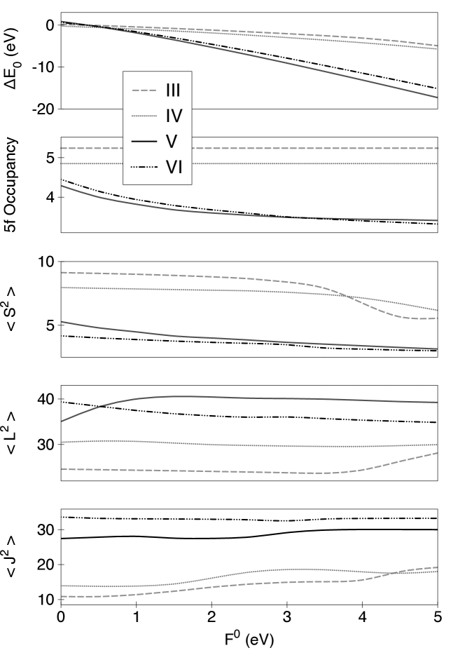
Figure 7: The correction to the DFT ground state energy, the occupancy of the 5f Löwdin orbitals, the total spin $\langle\vec{S}^{2}\rangle$ in the 5f orbitals, the total orbital angular momentum $\langle\vec{L}^{2}\rangle$ in the 5f orbitals, and the total angular momentum $\langle\vec{J}^{2}\rangle$ in the 5f orbitals as F⁰ is varied, holding $F^{2}$, $F^{4}$, and $F^{6}$ and the spin-orbit interaction fixed. The four oxidation states of plutonium are shown.

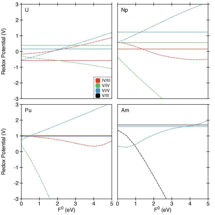
Figure 8: Calculated redox potentials of the actinide redox couples An(IV)/An(III) (red), An(V)/An(IV) (green), An(VI)/An(V) (blue) and Am(V)/Am(III) (black) as a function of $F^{0}$. Experimentally determined potentials are indicated by the solid horizontal lines.

The many-body correction to the ground state energy as computed within DFT changes the free energies of the reactions Eqs. 2 and 4 and hence the redox potentials. Fig. 8 shows the change in the redox potentials as a function of $F^{0}$. Potentials for $F^{0}=0$ are the DFT values corrected by the spin-orbit interaction and the Slater integrals $F^{2}$, $F^{4}$, and $F^{6}$. For the VI/V couples (shown in blue), the closest match with experiment is for $F^{0}=2.1$ eV (U), $1.3$ eV (Np), $0.4$ eV (Pu) and $3.7$ eV (Am). For the IV/III redox couples (red), the best match occurs for $F^{0}=1.4$ eV (Np) and $0.1$ eV (Pu) eV, but the correction to the electronic energies worsens the match to experiment in the case of U. However, in the case of the V/IV redox potentials (green), as well as the Am V/III potential (black), the pure DFT values are all low in comparison to experiment (see Fig. 3), and the corrections only lower the potentials further.

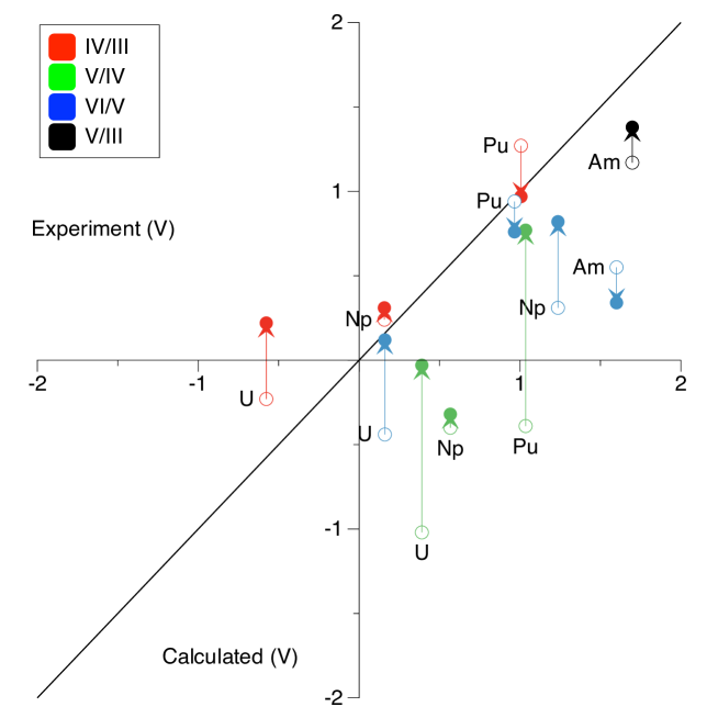
Figure 9: Many-body corrected redox potentials (filled symbols) compared to measured values. Open symbols are the potentials obtained from DFT including only the spin-orbit correction. $F^{0}=2.5$ eV for U(III) and U(IV); $1.0$ eV for Np(III) and (IV); $0.5$ eV for Pu(III) and (IV); and $0.5$ eV for Am(III). In each case $F^{0}$ is reduced by $0.5$ eV for oxidation states V and VI to account for increased screening of the Coulomb interaction in the actinyls.

As it stands the calculation does not account for changes in the screening of the Coulomb interaction as the oxidation state changes. A reduction in the size of $F^{0}$ for the actinyls yields in most cases a better match with experiment, particularly in the case of the V/IV redox couple. In Fig. 9 $F^{0}=2.5$ eV for U(III) and U(IV); $1.0$ eV for Np(III) and (IV); $0.5$ eV for Pu(III) and (IV); and $0.5$ eV for Am(III). In each case $F^{0}$ is reduced by $0.5$ eV for oxidation states V and VI. There is a striking improvement in the match with experiment with two exceptions: The calculated U IV/III and Am VI/V potentials move further away from the measured values. The downward shift in $F^{0}$ may reflect the role that the oxygen ligands play in screening repulsion between 5f electrons. A similar trend has been found in studies of isolated molecules and ions. For example in Ref. Norman:1995, a range of values for $F^{0}=2.3$ to $3.3$ eV are reported for an isolated U⁴⁺ ion, decreasing to $F^{0}=1.6$ eV in the case of the UPt₃ molecule.

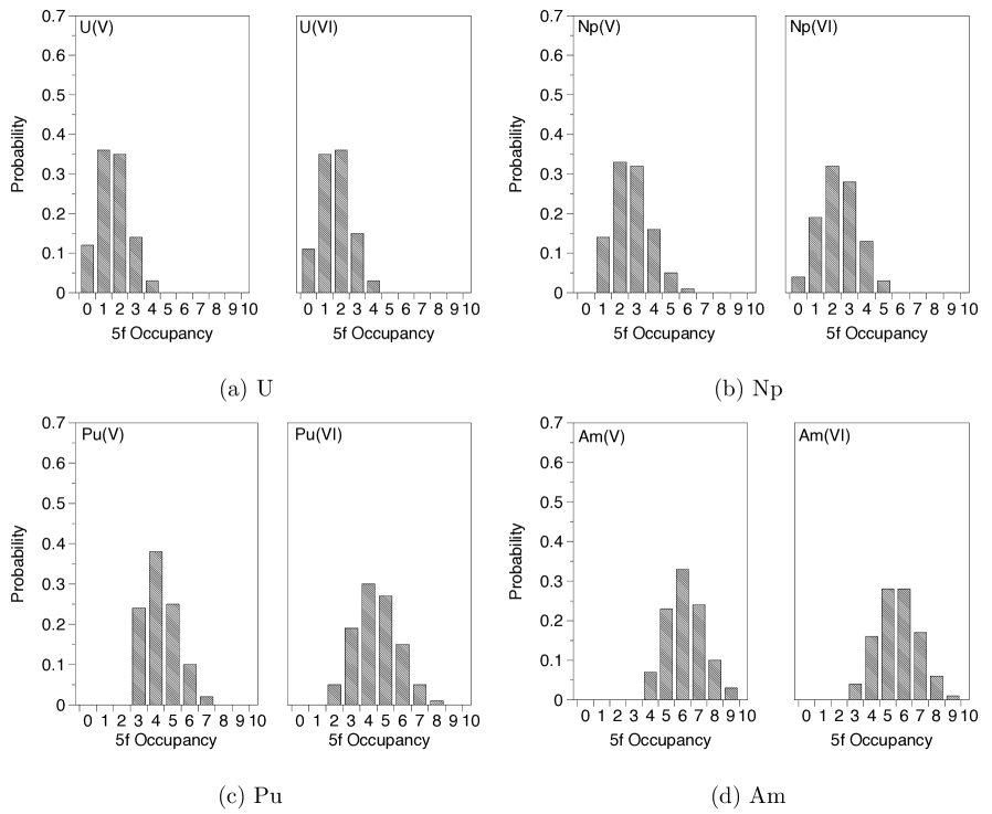
Figure 10: Histogram of the probability for different 5f electronic occupancies for oxidation states V and VI. $F^{0}$ has the same values as in Fig. 9.

Fig. 10 presents probability distributions of different electron occupanciesShim:2007p314 ; Yee:2010p452 in the actinyl 5f Löwdin orbitals, using the same values of $F^{0}$ adopted in Fig. 9. The distributions are particularly broad for neptunium and plutonium reflecting the increasing number of 5f electrons as one moves along the row of early actinides competing against an increasing tendency to localize.

VII Conclusion

The hybrid DFT / many-body approach taken in this paper shows some promise for the theoretical modeling of the difficult but important problem of redox chemistry involving the early actinide elements. By incorporating the physics of strong correlations between electrons in the frontier orbitals we are able to correct the electronic contribution to the free energy as computed in DFT, and thereby bring the calculated redox potentials into closer agreement with measured values. The calculations require one adjustable parameter, $F^{0}$, for each actinide species, in addition to a $0.5$ eV downshift in $F^{0}$ for the actinyls, yet has predictive power as it yields potentials for 3 redox couples An(VI)/An(V), An(V)/An(IV), and An(IV)/An(III).

The match with experiment is improved in 6 of the 11 redox reactions that we study; agreement remains good in the case of 2 reactions (Pu VI/V and Np IV/III), little changed but poor for Np V/IV, and worsens for 2 others (U IV/III and Am VI/V. The calculated potentials are certainly not of chemical accuracy, but they do evidence significant trends. In the case of plutonium, for instance, the calculated potentials approach the measured near-degeneracy of the 3 redox potentials, and hence go some distance towards explaining the propensity of plutonium species in solution to easily disproportionate and co-exist in several different oxidation states.Clark:2000 In the language of Hubbard models, disproportionation may be viewed as a consequence of an effective negative-U interaction for the overall complex; see for instance Refs. Watkins:1984, ; vanderMarel:1988p330, ; Harrison:2006p316, . In our calculations its origin may be traced in part to the strong correlations between the 5f electrons that permit the electrons to avoid each other more efficiently than they can at the level of LDA/GGA or HF, lowering the electronic energy. When combined with all the other contributions to the free energy (solvation, vibrations, and translations) the redox potentials become degenerate and an overall effective negative-U interaction emerges.

The calculations can be improved or extended in several ways. At the DFT level, different geometries with varying numbers of water molecules in the solvation spheres can be investigated. It may be desirable to treat a second sphere of solvation quantum mechanically rather than with continuum dielectric models. Of geochemical interest is actinide complexation with carbonate and silicate substrates, and with colloids,Clark:2000 ; Kubicki:2009p125 and these could be investigated by the hybrid approach. The projection onto Löwdin orbitals could be replaced with projective orthogonalizationToropova:2007 to better minimize the admixture of neglected orbitals. It may be possible to include some additional orbitals in the many-body model, if not by exact diagonalization then possibly by methods such as the density-matrix renormalization-group (DMRG). It would also be interesting to investigate the problem of double-counting the interaction in the hybrid approach by carrying out a pure HF calculation, working directly with the physical electrons rather than with KS fermions. However it is expected that the pure HF calculation will not by itself be a sufficiently accurate foundation for free energy calculations. Ultimately it would be desirable to replace hybrid DFT / Anderson impurity model approach developed here with a unified first principles method that can simultaneously and accurately describe the physics and chemistry of relativity, solvation, and strong electronic correlations.

- (1) T. Fanghänel and V. Neck, Pure Appl. Chem. 74, 1895 (2002).
- (2) G. R. Choppin and A. Morgenstern, in Radioactivity in the Environment: Plutonium in the Environment, Vol. 1, edited by A. Kudo (Elsevier, Amsterdam, 2001).
- (3) D. L. Clark, Los Alamos Science 26, 364 (2000).
- (4) E. Runge, P. Fulde, D. Efremov, N. Hasselmann, and G. Zwicknagl, Physical Review B 69, 155110 (2004).
- (5) G. Schreckenbach and G. Shamov, Accounts of Chemical Research 43, 19 (2010), http://pubs.acs.org/doi/abs/10.1021/ar800271r.
- (6) J. Roberto, T. D. de la Rubia, R. Gibala, and S. Zinkle, Report of the Basic Energy Sciences Workshop on Basic Research Needs for Advanced Nuclear Energy Systems (US DOE, 2006) http://dx.doi.org/10.1007/s11837-007-0048-x.
- (7) J. Straus, A. Calhoun, and G. Voth, The Journal of Chemical Physics 102, 529 (1995).
- (8) A. Hubsch, J. C. Lin, J. Pan, and D. L. Cox, Phys. Rev. Lett. 96, 196401 (2006), http://link.aps.org/abstract/PRL/v96/e196401.
- (9) M. X. LaBute, R. V. Kulkarni, R. G. Endres, and D. L. Cox, J. Chem. Phys. 116, 3681 (2002).
- (10) M. X. LaBute, R. G. Endres, and D. L. Cox, J. Chem. Phys. 121, 8221 (2004).
- (11) J. B. Marston, D. R. Andersson, E. R. Behringer, B. H. Cooper, C. A. DiRubio, G. A. Kimmel, and C. Richardson, Physical Review B 48, 7809 (1993).
- (12) A. V. Onufriev and J. B. Marston, Physical Review B 53, 13340 (1996).
- (13) R. Bartlett and M. Musiał, Rev. Mod. Phys. 79, 291 (2007).
- (14) G. Schreckenbach, P. J. Hay, and R. L. Martin, Inorg. Chem. 37, 4442 (1998), http://pubs.acs.org/doi/abs/10.1021/ic980057a.
- (15) S. Spencer, L. Gagliardi, N. Handy, A. Ioannou, C.-K. Skylaris, A. Willetts, and A. Simper, J. Phys. Chem. A 103, 1831 (1999).
- (16) J. Blaudeau, S. Zygmunt, L. Curtiss, D. Reed, and B. Bursten, Chemical Physics Letters 310, 347 (1999).
- (17) P. J. Hay, R. L. Martin, and G. Schreckenbach, J. Phys. Chem. A 104, 6529 (2000).
- (18) S. Tsushima, T. Yang, and A. Suzuki, Chemical Physics Letters 334, 365 (2001).
- (19) V. Vallet, U. Wahlgren, B. Schimmelpfennig, H. Moll, Z. Szabo, and I. Grenthe, Inorganic Chemistry 40, 3516 (2001).
- (20) V. Vallet, T. Privalov, U. Wahlgren, and I. Grenthe, J. Am. Chem. Soc. 126, 7766 (2004).
- (21) S. Tsushima and T. Yang, Chemical Physics Letters 401, 68 (2005).
- (22) J. L. Sonnenberg, P. J. Hay, R. L. Martin, and B. E. Bursten, Inorg. Chem. 44, 2255 (2005), http://pubs.acs.org/doi/abs/10.1021/ic048567u.
- (23) Z. Cao and K. Balasubramanian, J. Chem. Phys. 123, 114309 (2005).
- (24) G. Shamov and G. Schreckenbach, J. Phys. Chem. A 109, 10961 (2005).
- (25) K. Gutowski and D. Dixon, J. Phys. Chem. A 110, 8840 (2006).
- (26) W. Kuchle, M. Dolg, H. Stoll, and H. Preuss, J. Chem. Phys. 100, 7535 (1994).
- (27) S. Odoh and G. Schreckenbach, J. Phys. Chem. A 114, 1957 (2010).
- (28) SCM, “ADF2009.01,” Theoretical Chemistry, Vrije Universiteit, Amsterdam, The Netherlands (2009), www.scm.com.
- (29) E. van Lenthe, E. Baerends, and J. Snijders, J. Chem. Phys. 99, 4597 (1993).
- (30) E. van Lenthe, The ZORA Equation, Ph.D. thesis, University of Amsterdam (1996).
- (31) A. Klamt, J. Phys. Chem. 99, 2224 (1995).
- (32) B. Hammer, L. B. Hansen, and J. K. Norskov, Phys. Rev. B 59, 7413 (1999), http://dx.doi.org/10.1103/PhysRevB.59.7413.
- (33) J. P. Perdew, K. Burke, and M. Ernzerhof, Phys. Rev. Lett. 77, 3865 (1996), http://dx.doi.org/10.1103/PhysRevLett.77.3865.
- (34) S. H. Vosko, L. Wilk, and M. Nusair, Can. J. Phys. 58, 1200 (1980).
- (35) R. L. Martin, P. J. Hay, and L. R. Pratt, J. Phys. Chem. A 102, 3565 (1998).
- (36) M. Denecke, K. Dardenne, and C. Marquardt, Talanta 65, 1008 (2005).
- (37) S. D. Conradson, Appl. Spectrosc. 52, 252A (1998).
- (38) P. Allen, J. Bucher, D. Shuh, N. Edelstein, and T. Reich, Inorg. Chem. 36, 4676 (1997).
- (39) D. L. Clark, in The Convergence of Theory and Experiment (Presented at the Symposium on Heavy Element Complexes, 217th ACS National Meeting, Anaheim, CA, 1999).
- (40) C. D. Tait, in The Convergence of Theory and Experiment (Presented at the Symposium on Heavy Element Complexes, 217th ACS National Meeting, Anaheim, CA, 1999).
- (41) U. Wahlgren, H. Moll, I. Grenthe, B. Schimmelpfennig, L. Maron, V. Vallet, and O. Gropen, J. Phys. Chem. A 103, 8257 (1999).
- (42) M. Aaberg, D. Ferri, J. Glaser, and I. Grenthe, Inorg. Chem. 22, 3986 (1983).
- (43) S. Cotton, Lanthanide and Actinide Chemistry (John Wiley and Sons, Ltd., 2006).
- (44) P. Allen, J. Bucher, D. Shuh, N. Edelstein, and I. Craig, Inorg. Chem. 39, 595 (2000).
- (45) S. G. Bratsch, J. Phys. Chem. Ref. Data 18, 1 (1989), http://dx.doi.org/10.1063/1.555839.
- (46) S. Kihara, Z. Yoshida, H. Aoyagl, H. Maeda, Osamu, Shirai, Y. Kitatsuji, and Y. Yoshida, Pure and Applied Chemistry 71, 1771 (1999).
- (47) G. Shamov and G. Schreckenbach, Journal of Physical Chemistry A 110, 12072 (2006), http://www.cheric.org/research/tech/periodicals/vol_view.php?seq=566857%.
- (48) D. Clark, S. Hecker, G. Jarvinen, and M. Neu, Kirk-Othmer Encyclopedia of Chemical Technology 19, 667 (2006), http://onlinelibrary.wiley.com/doi/10.1002/0471238961.1612212013151819.%a01.pub2/full.
- (49) P.-O. Löwdin, J. Chem. Phys. 18, 365 (1950).
- (50) J. A. Gaunt, Phil. Trans. R. Soc. London A 228, 151 (1929).
- (51) G. Racah, Phys. Rev. 62, 438 (1942), http://dx.doi.org/10.1103/PhysRev.62.438.
- (52) J. C. Slater, Phys. Rev. 34, 1293 (1929), http://dx.doi.org/10.1103/PhysRev.34.1293.
- (53) E. U. Condon and G. H. Shortley, Phys. Rev. 37, 1025 (1931), http://dx.doi.org/10.1103/PhysRev.37.1025.
- (54) M. R. Norman, Phys. Rev. B 52, 1421 (1995), http://dx.doi.org/10.1103/PhysRevB.52.1421.
- (55) R. C. Albers, N. E. Christensen, and A. Svane, Journal of Physics: Condensed Matter 21, 343201 (2009), 0907.1028v1, http://arxiv.org/abs/0907.1028v1.
- (56) B. Veal, D. Lam, H. Diamond, and H. Hoekstra, Phys. Rev. B 15, 2929 (1977).
- (57) J. Shim, K. Haule, and G. Kotliar, Nature 446, 513 (2007).
- (58) C.-H. Yee, G. Kotliar, and K. Haule, Physical Review B 81, 035105 (2010).
- (59) G. Watkins, in Festrperprobleme (Advances in Solid State Physics), Vol. XXIV, edited by P. Grosee (Vieweg, Braunschweig, 1984) pp. 163–189.
- (60) D. van der Marel and G. A. Sawatzky, Physical Review B (Condensed Matter) 37, 67188 (1988), http://adsabs.harvard.edu/cgi-bin/nph-data_query?bibcode=1988PhRvB..371%0674V&link_type=ABSTRACT.
- (61) W. Harrison, Physical Review B 74, 245128 ( 2006).
- (62) J. Kubicki, G. Halada, P. Jha, and B. Phillips, Chemistry Central Journal 3, 10 (2009).
- (63) A. Toropova, C. A. Marianetti, K. Haule, and G. Kotliar, Phys. Rev. B 76, 155126 (2007), http://link.aps.org/abstract/PRB/v76/e155126.