Photoacoustic Imaging Taking into Account Attenuation

1 Introduction

Photoacoustic Imaging is one of the recent hybrid imaging techniques, which attempts to visualize the distribution of the electromagnetic absorption coefficient inside a biological object. In photoacoustic experiments, the medium is exposed to a short pulse of a relatively low frequency electromagnetic (EM) wave. The exposed medium absorbs a fraction of the EM energy, heats up, and reacts with thermoelastic expansion. This induces acoustic waves, which can be recorded outside the object and used to determine the electromagnetic absorption coefficient. The combination of EM and ultrasound waves (which explains the usage of the term hybrid) allows one to combine high contrast in the EM absorption coefficient with high resolution of ultrasound. The method has demonstrated great potential for biomedical applications, including functional brain imaging of animals WPKXS (03), soft-tissue characterization, and early stage cancer diagnostics KKMR (00), as well as imaging of vasculature ZLB (07). For a general survey on biomedical applications see XW (06). In comparison with the X-Ray CT, photoacoustics is non-ionizing. Its further advantage is that soft biological tissues display high contrasts in their ability to absorb frequency electromagnetic waves. For instance, for radiation in the near infrared domain, as produced by a Nd:YAG laser, the absorption coefficient in human soft tissues varies in the range of $0.1/\textrm{cm}$–$0.5/\textrm{cm}$ CPW (90). The contrast is also known to be high between healthy and cancerous cells, which makes photoacoustics a promising early cancer detection technique. Another application arises in biology: Multispectral optoacoustic tomography technique is capable of high-resolution visualization of fluorescent proteins deep within highly light-scattering living organisms RDVMPKN . In contrast, the current fluorescence microscopy techniques are limited to the depth of several hundred micrometers, due to intense light scattering.

Different terms are often used to indicate different excitation sources: Optoacoustics refers to illumination in the visible light spectrum, Photoacoustics is associated with excitations in the visible and infrared range, and Thermoacoustics corresponds to excitations in the microwave or radio-frequency range. In fact, the carrier frequency of the illuminating pulse is varying, which is usually not taken into account in mathematical modeling. Since the corresponding mathematical models are equivalent, in the mathematics literature, the terms opto-, photo-, and thermoacoustics are used interchangeably. In this article, we are addressing only the photoacoustic tomographic technique PAT (which is mathematically equivalent to the thermoacoustic tomography TAT).

Various kinds of photoacoustic imaging techniques have been implemented. One should distinguish between photoacoustic microscopy (PAM) and tomography (PAT). In microscopy, the object is scanned pixel by pixel (or voxel by voxel). The measured pressure data provides an image of the electromagnetic absorption coefficient ZMSW (06). Tomography, on the other hand, measures pressure waves with detectors surrounding completely or partially the object. Then the internal distribution of the absorption coefficients is reconstructed using mathematical inversion techniques (see the sections below).

The common underlying mathematical equation of PAT is the wave equation for the pressure

$$\boxed{\frac{1}{c_{0}^{2}}\frac{\partial^{2}p}{\partial t^{2}}({\vec{x}},t)-\nabla^{2}p({\vec{x}},t)=\frac{dj}{dt}(t)\left(\frac{\mu_{\rm abs}({\vec{x}})\beta({\vec{x}})J({{\vec{x}}})}{c_{p}({\vec{x}})}\right)\,,\;{\vec{x}}\in{\mathbb{R}}^{3},\,t>0\;.}$$ (1)

Here $c_{p}$ denotes the specific heat capacity, $J$ is the spatial intensity distribution, $\mu_{\rm abs}$ denotes the absorption coefficient, $\beta$ denotes the thermal expansion coefficient and $c_{0}$ denotes the speed of sound, which is commonly assumed to be constant. The assumption that there is no acoustic pressure before the object is illuminated at time $t=0$ is expressed by

$$\boxed{p({\vec{x}},t)=0\,,\qquad{\vec{x}}\in{\mathbb{R}}^{3},t<0\;.}$$ (2)

In PAT, $j(t)$ approximates a pulse, and can be considered as a $\delta$-impulse $\delta(t)$. Introducing the shorthand notations

$$\rho({\vec{x}}):=\frac{\mu_{\rm abs}({\vec{x}})\beta({\vec{x}})J({\vec{x}})}{c_{p}({\vec{x}})}\,,$$ (3)

one reduces (1) and (2) to

$$\boxed{\frac{1}{c_{0}^{2}}\frac{\partial^{2}p}{\partial t^{2}}({\vec{x}},t)-\nabla^{2}p({\vec{x}},t)=0\,,\quad{\vec{x}}\in{\mathbb{R}}^{3},t>0\,,}$$ (4)

with initial values

$$\boxed{p({\vec{x}},0)=\rho({\vec{x}})\,,\quad\frac{\partial p}{\partial t}({\vec{x}},0)=0\qquad{\vec{x}}\in{\mathbb{R}}^{3}\;.}$$ (5)

The quantity $\rho$ in (1) and (3) is a combination of several physical parameters. All along this paper $\rho$ should not be confused with the source term

$$\boxed{f({\vec{x}},t)=\frac{dj}{dt}(t)\rho({\vec{x}})\,,\quad{\vec{x}}\in{\mathbb{R}}^{3},t>0\;.}$$ (6)

In PAT, some data about the pressure $p({\vec{x}},t)$ are measured and the main task is to reconstruct the initial pressure $\rho$ from these data. While the excitation principle is always as described above and thus (4) holds, the specific type of data measured depends on the type of transducers used, and thus influences the mathematical model.

Nowadays there is a trend to incorporate more and more modeling into photoacoustic. In particular, taking into account locally varying wave speed and attenuation. Even more there is a novel trend to qualitative photoacoustics, which is concerned with estimating physical parameters from the imaging parameter of standard photoacoustics. In this paper we focus on attenuation correction, where we survey some recent progress. Inversion with varying wave speed has been considered for instance in AK (07); HKN (08), and is not further discussed here.

The outline of this paper is as follows: First, we review existing attenuation models and discuss their causality properties, which we believe to be essential for algorithms for inversion with attenuated data. Then, we survey causality properties of common attenuation models. We also derive integro-differential equations which the attenuated waves are satisfying. In addition we discuss the ill–conditionness of the inverse problem for calculating the unattenuated wave from the attenuated one.

2 Attenuation

The difficult issue of effects of and corrections for the attenuation of acoustic waves in PAT has been studiedRZA (06); BGHNP (07); PG (06); KSB (10), although no complete conclusion on the feasibility of these models has been reached.

Mathematical models for describing attenuation are formulated in the frequency domain, taking into account that attenuation disperses high frequency components more rapidly over traveled distance. Let $\mathcal{G}({\vec{x}},t)$ denote the attenuated wave which originates from an impulse ($\delta_{{\vec{x}},t}$-distribution) at ${\vec{x}}=0$ at time $t=0$. In mathematical terms $\mathcal{G}$ is the Green-function of attenuated wave equation. Moreover, we denote by

$$\boxed{\mathcal{G}_{0}({\vec{x}},t)=\frac{\delta\left(t-\frac{\left|{\vec{x}}\right|}{c_{0}}\right)}{4\,\pi\,\left|{\vec{x}}\right|}}$$ (7)

the Green function of the unattenuated wave equation; that is, it is the solution of (4), (5) with constant sound speed $c(x)\equiv c_{0}$ and initial conditions

$$\mathcal{G}_{0}({\vec{x}},0)=0\quad\mbox{ and}\quad\frac{\partial\mathcal{G}_{0}}{\partial t}({\vec{x}},0)=\delta_{{\vec{x}},t}\,.$$

Common mathematical formulations of attenuation assume that

$$\boxed{\mathcal{F}\left\{\mathcal{G}\right\}({\vec{x}},\omega)=\exp\left(-\beta^{*}(\left|{\vec{x}}\right|,\omega)\right)\,\mathcal{F}\left\{\mathcal{G}_{0}\right\}({\vec{x}},\omega)\,,\quad{\vec{x}}\in{\mathbb{R}}^{3},\,\omega\in{\mathbb{R}}\;.}$$ (8)

Here $\mathcal{F}\left\{\cdot\right\}$ denotes the Fourier transform with respect to time $t$ (cf. Appendix 8). Applying the inverse Fourier transform $\mathcal{F}^{-1}\left\{\cdot\right\}$ to (8) gives

$$\boxed{\mathcal{G}({\vec{x}},t)=K({\vec{x}},t)*_{t}\mathcal{G}_{0}({\vec{x}},t)}\qquad\mbox{($*_{t}$ time convolution)}$$ (9)

where

$$K({\vec{x}},t):=\frac{1}{\sqrt{2\,\pi}}\mathcal{F}^{-1}\left\{\exp\left(-\beta^{*}(\left|{\vec{x}}\right|,\cdot)\right)\right\}(t)\;.$$ (10)

From (9) and (7) it follows that

$$\mathcal{G}({\vec{x}},t) =K({\vec{x}},t)*_{t}\mathcal{G}_{0}({\vec{x}},t)$$

$$=\int_{\mathbb{R}}K({\vec{x}},t-\tau)\frac{\delta(\tau-\frac{\left|{\vec{x}}\right|}{c_{0}})}{4\pi\left|{\vec{x}}\right|}\,d\tau$$

$$=\frac{K\left({\vec{x}},t-\frac{\left|{\vec{x}}\right|}{c_{0}}\right)}{4\pi\left|{\vec{x}}\right|}\;.$$

Consequently,

$$\boxed{\mathcal{G}({\vec{x}},t+\left|{\vec{x}}\right|/c_{0})=K({\vec{x}},t)/(4\pi\left|{\vec{x}}\right|)\;.}$$ (11)

Moreover, we emphasize that the Fourier transform of a real and even (real and odd) function is real and even (imaginary and odd). Since $\mathcal{G}$ and $\mathcal{G}_{0}$ are real valued, $K$ must be real valued and consequently the real part $\Re(\beta^{*})$ of $\beta^{*}$ has to be even with respect to the frequency $\omega$ and $\Im(\beta^{*})$ has to be odd with respect to $\omega$. Attenuation is caused if $\Re(\beta^{*})$ is positive and since then $\beta^{*}$ has a nonzero imaginary part due to the Kramers-Kronig relation, attenuation causes dispersion. In the literature the following product ansatz is commonly used

$$\boxed{\beta^{*}(\left|{\vec{x}}\right|,\omega)=\alpha^{*}(\omega)\,\left|{\vec{x}}\right|\qquad\omega\in{\mathbb{R}},\,{\vec{x}}\in{\mathbb{R}}^{3}\;.}$$ (12)

In the sequel we concentrate on these models and use the following terminology:

Definition 1

We call $\beta^{*}$ of standard form if (12) holds. Then the function

$$\alpha^{*}:{\mathbb{R}}\to{\mathbb{C}}$$ (13)

is called standard attenuation coefficient and $\alpha=\Re(\alpha^{*})$ is called the attenuation law. We also call $\beta^{*}$ the attenuation coefficient.

From the relation (12), it follows that $\Re(\alpha^{*})$ is even, $\Im(\alpha^{*})$ is odd, and $\Re(\alpha^{*})>0$ (the last inequality guarantees attenuation).

In the following we summarize common attenuation coefficients and laws: In what follows $\alpha_{0}$ denotes a positive parameter and

$$\tilde{\alpha}_{0}=\frac{\alpha_{0}}{\cos\left(\frac{\pi}{2}\gamma\right)}\qquad\quad(0<\gamma\not\in{\mathbb{N}})\,$$ (14)

is a possibly non-positive coefficient.

• Frequency Power Laws:

  • Let $0<\gamma\not\in{\mathbb{N}}$. The frequency power law attenuation coefficient is defined by

    $$\alpha_{pl}^{*}(\omega)=\tilde{\alpha}_{0}(-{\mathrm{i}}\,\omega)^{\gamma}=\tilde{\alpha}_{0}\left|\omega\right|^{\gamma}\left(\cos\left(\frac{\pi}{2}\gamma\right)-{\mathrm{i}}\,\mbox{sgn}(\omega)\sin\left(\frac{\pi}{2}\gamma\right)\right)$$ (15)

    for $\omega\in{\mathbb{R}}$. Therefore, the attenuation law is given by

    $$\boxed{\alpha_{pl}(\omega)=\alpha_{0}\,\left|\omega\right|^{\gamma}\;.}$$ (16)

    These models have been considered for instance in S (94, 95); WHBM (00); WMM (05).

  • Let $\gamma=1$ and $\omega_{0}\neq 0$, the attenuation coefficient is defined by

    $$\alpha_{pl}^{*}(\omega):=\alpha_{0}\,\left|\omega\right|+{\mathrm{i}}\,\frac{2}{\pi}\,\alpha_{0}\,\omega\,\log\left|\frac{\omega}{\omega_{0}}\right|\qquad\omega\in{\mathbb{R}}\,.$$ (17)

    The attenuation law is

    $$\boxed{\alpha_{pl}(\omega):=\alpha_{0}\,\left|\omega\right|\;.}$$ (18)

    This model has been considered in S (95); WMM (05).

• Szabo: Let $0<\gamma\not\in{\mathbb{N}}$. The attenuation coefficient of Szabo’s law is defined by

  $$\alpha_{sz}^{*}(\omega) =\frac{1}{c_{0}}\,\sqrt{(-{\mathrm{i}}\,\omega)^{2}+2\tilde{\alpha}_{0}c_{0}(-{\mathrm{i}}\,\omega)^{\gamma+1}}+{\mathrm{i}}\,\frac{\omega}{c_{0}}\;.$$ (19)

  We denote Szabo’s attenuation law by

  $$\boxed{\alpha_{sz}(\omega):=\Re(\alpha_{sz}^{*}(\omega))\;.}$$

  For small frequencies $\alpha_{sz}(\omega)$ behaves like $\alpha_{0}\,|\omega|^{\gamma}$. This model has been considered in S (94, 95) where, in addition, also a model for $\gamma\in{\mathbb{N}}$ has been introduced.

• Thermo-Viscous Attenuation Law: (see e.g. KFCS (00); S (94)): Here, for $\tau_{0}>0$, the attenuation coefficient is defined by

  $$\alpha_{tv}^{*}(\omega)=\frac{-{\mathrm{i}}\,\omega}{c_{0}\,\sqrt{1-{\mathrm{i}}\,\tau_{0}\,\omega}}+\frac{{\mathrm{i}}\,\omega}{c_{0}}$$ (20)

  with attenuation law

  $$\boxed{\alpha_{tv}(\omega)=\frac{\tau_{0}\,\omega^{2}}{\sqrt{2}\,c_{0}\,\sqrt{(1+\sqrt{1+(\tau_{0}\,\omega)^{2}})\,(1+(\tau_{0}\,\omega)^{2})}}\;.}$$ (21)

  For small frequencies $\alpha_{tv}(\omega)$ behaves like $\frac{\tau_{0}\,\omega^{2}}{2\,c_{0}}$. That is the thermo-viscous law approximates a power attenuation law with exponent $2$.

• Nachman, Smith and Waag NSW (90): Consider a homogeneous and isotropic fluid with density $\rho_{0}$ in which $N$ relaxation processes take place. Then the attenuation coefficient of the model in NSW (90) reads as follows:

  $$\alpha_{nsw}^{*}(\omega)=\frac{-{\mathrm{i}}\,\omega}{c_{0}}\,\left[\frac{c_{0}}{\tilde{c}_{0}}\,\sqrt{\frac{1}{N}\,\sum_{m=1}^{N}\frac{1-{\mathrm{i}}\,\,\tilde{\tau}_{m}\,\omega}{1-{\mathrm{i}}\,\tau_{m}\,\omega}}-1\right]\;.$$ (22)

  All parameters appearing in (22) are positive and real. $\kappa_{m}$ and $\tau_{m}$ denote the compression modulus and the relaxation time of the $m-$th relaxation process, respectively, and

  $$\tilde{c}_{0}:=\frac{c_{0}}{\sqrt{1+\sum_{m=1}^{N}c_{0}^{2}\,\rho_{0}\,\kappa_{m}}}\quad\mbox{and}\quad\tilde{\tau}_{m}:=\tau_{m}\,(1-N\,\tilde{c}_{0}^{2}\,\rho_{0}\,\kappa_{m})\,.$$ (23)

  The last two definitions imply that

  $$\frac{\tilde{c}_{0}^{2}}{c_{0}^{2}}=\frac{1}{N}\,\sum_{m=1}^{N}\frac{\tilde{\tau}_{m}}{\tau_{m}}\;.$$ (24)

  We denote the according attenuation law by

  $$\boxed{\alpha_{nsw}(\omega):=\Re(\alpha_{nsw}^{*}(\omega))\;.}$$

• Greenleaf and Patch PG (06) consider for $\gamma\in\{1,2\}$ the attenuation coefficient

  $$\alpha_{gp}^{*}(\omega)=\alpha_{0}\,\left|\omega\right|^{\gamma}\,,$$

  which, since it is real, equals the attenuation law

  $$\boxed{\alpha_{gp}(\omega)=\Re(\alpha_{gp}^{*}(\omega))\;.}$$ (25)

• Chen and Holm CH (04): This model describes the attenuation as a function of the absolute value of the vector-valued wave number $\mathbf{k}\in{\mathbb{R}}^{3}$ (instead of the frequency $\omega\in{\mathbb{R}}$). Let $\mathcal{F}_{3D}$ denote the $3D-$Fourier transform

  $$\mathcal{F}_{3D}\{f(\mathbf{k})\}({\vec{x}})=\frac{1}{\sqrt{(2\,\pi)^{3}}}\,\int_{{\mathbb{R}}^{3}}\exp\left({\mathrm{i}}\,{\vec{x}}\cdot\mathbf{k}\right)\,f(\mathbf{k})\,\mbox{d}\mathbf{k}\,,$$

  then the Green function of the attenuated equation is defined by

  $$\mathcal{G}({\vec{x}},t)=\frac{H(t)\,c_{0}^{2}}{(2\,\pi)^{3/2}}\,\mathcal{F}_{3D}\left\{\exp\left(A(\cdot)\,t\right)\,\frac{\sin(B(\cdot)\,t)}{B(\cdot)}\right\}({\vec{x}})$$ (26)

  where, for given $\alpha_{1}>0$,

  $$A(\mathbf{k}):=-\alpha_{1}\,c_{0}\,\left|\mathbf{k}\right|^{\gamma}\,,\qquad B(\mathbf{k}):=c_{0}\,\sqrt{\left|\mathbf{k}\right|^{2}-\alpha_{1}^{2}\,\left|\mathbf{k}\right|^{2\,\gamma}}\,.$$ (27)

• In KSB (10) we proposed

  $$\alpha_{ksb}^{*}(\omega)=\frac{\alpha_{0}\,(-{\mathrm{i}}\,\omega)}{c_{0}\,\sqrt{1+(-{\mathrm{i}}\,\tau_{0}\,\omega)^{\gamma-1}}}\qquad\qquad(\gamma\in(1,2],\,\tau_{0}>0)\,,$$ (28)

  where the square root is again the complex root with positive real part.

  Let $\gamma\in(1,2]$. Then, for small frequencies we have

  $$\boxed{\alpha_{ksb}(\omega)\approx\frac{\alpha_{0}\,\sin(\frac{\pi}{2}(\gamma-1))}{2\,c_{0}\,\tau_{0}}\,|\tau_{0}\,\omega|^{\gamma}>0\,.}$$

  Thus our model behaves like a power law for small frequencies.

Distinctive features of unattenuated wave propagation (,i.e. the solution of the standard wave equation) are causality and finite wave front velocity. It is reasonable to assume that the attenuated wave satisfies the same distinctive properties as well. In the following we analyze causality properties of the standard attenuation models.

3 Causality

In the following we present some abstract definitions and basic notations. In the remainder ${\vec{x}}$ will always denote a vector in three dimensional space. When we speak about functions, we always mean generalized functions, such as for instance distributions or tempered distributions - we recall the definitions of (tempered) distribution in the course of the paper.

Definition 2

A function $f:=f({\vec{x}},t)$ defined on the Euclidean space over time (i.e. in ${\mathbb{R}}^{4}$) is said to be causal if it satisfies $f({\vec{x}},t)=0$ for $t<0$.

Notation & Terminology 3.1

Let $\mathcal{A}:D\to D$ be a linear operator, where $\emptyset\neq D$ is an appropriate set of functions from ${\mathbb{R}}^{4}$ to ${\mathbb{R}}$. In this paper we always assume that $\mathcal{A}$ satisfies the following properties:

• $\mathcal{A}$ is shift invariant in space and time. That is, for every function $f$ and every shift $L:=L({\vec{x}},t):=({\vec{x}}-{\vec{x}}_{0},t-t_{0})$, with ${\vec{x}}_{0}\in{\mathbb{R}}^{3}$ and $t_{0}\in{\mathbb{R}}$, it holds that

  $$\mathcal{A}(f\circ L)=(\mathcal{A}f)\circ L\;.$$

• $\mathcal{A}$ is rotation invariant in space. That is, for every function $f$ and every rotation matrix $R$, it holds that

  $$\mathcal{A}(Rf)=R(\mathcal{A}f)\;.$$

• $\mathcal{A}$ is causal. That is, it maps causal functions to causal functions. From (29) it follows that $\mathcal{A}$ is causal, if and only if the associated Green function is causal.

Definition 3

The Green function of $\mathcal{A}$ is defined by

$$\mathcal{G}:=\mathcal{G}({\vec{x}},t)=\mathcal{A}\delta_{{\vec{x}},t}({\vec{x}},t)\;.$$

Remark 1

The operator $\mathcal{A}$ is uniquely determined by $\mathcal{G}$ and vice versa. This follows from the fact that

$$\mathcal{A}f({\vec{x}}_{0},t_{0}) =\mathcal{A}\left(\int_{\mathbb{R}}\int_{{\mathbb{R}}^{3}}f({\vec{x}}_{0}-{\vec{x}},t-t_{0})\delta_{{\vec{x}},t}({\vec{x}},t)\,d{\vec{x}}dt\right)$$ (29)

$$=\int_{\mathbb{R}}\int_{{\mathbb{R}}^{3}}f({\vec{x}}_{0}-{\vec{x}},t-t_{0})\mathcal{G}({\vec{x}},t)\,d{\vec{x}}dt\,.$$

Moreover, we use the following terminology and abbreviations:

• From the rotation invariance of $\mathcal{A}$ it follows that

  $$\hat{T}({\vec{x}}):=\sup\{t:\mathcal{G}({\vec{x}},\tau)=0\text{ for all }\tau\leq t\}\,,$$ (30)

  is rotationally symmetric, which allows us to use the shorthand notation

  $$T(r)=\hat{T}({\vec{x}})\text{ where }r=\left|{\vec{x}}\right|\;.$$ (31)

  With this notation (30) can be equivalently expressed as

  $$\mathcal{G}\left({\vec{x}},t+T(\left|{\vec{x}}\right|)\right)=0\text{ for every }t<0\;.$$ (32)

  In physical terms $T(\left|{\vec{x}}\right|)$ denotes the travel time of a wave front originating at position $\mathbf{0}$ at time $t=0$ and traveling to ${\vec{x}}$.

• Because $\mathcal{G}$ is rotationally symmetric we can write

  $$\mathcal{G}({\vec{x}},T(\left|{\vec{x}}\right|))=\hat{\mathcal{G}}(r,T(r))\text{ with }r=\left|{\vec{x}}\right|\;.$$

  Taking the inverse function of $T$, which we denote by $S=S(t)$, we then find

  $$\mathcal{G}({\vec{x}},T(\left|{\vec{x}}\right|))=\hat{\mathcal{G}}(S(t),t)\,,$$

• The wave front is the set

  $${\cal W}:=\{({\vec{x}},T(\left|{\vec{x}}\right|)):{\vec{x}}\in{\mathbb{R}}^{3}\}\;$$

• The wave front speed $V$ is the variation of the location of the wave front as a function of time. That is,

  $$V(t)=\frac{\mbox{d}S}{\mbox{d}t}(t)=\left.\frac{1}{T^{\prime}(r)}\right|_{r=S(t)}\,.$$ (33)

  Here $T^{\prime}$ denotes the derivative with respect to the radial component $r$.

• We say that $\mathcal{A}$ has a finite speed of propagation if there exists a constant $\hat{c}_{0}$ such that

  $$0<\left(T^{\prime}(r)\right)^{-1}\leq\hat{c}_{0}<\infty\;.$$ (34)

  In this case it follows from (33) that the wave front velocity satisfies

  $$V(t)\leq\hat{c}_{0}<\infty\;.$$ (35)

• We call an operator $\mathcal{A}$ strongly causal, if it is causal and satisfies the finite propagation speed property.

The following lemma addresses the case of attenuation coefficients of standard form and gives examples of strongly causal operators $\mathcal{A}$.

Lemma 1

Let $\beta^{*}(\left|{\vec{x}}\right|,\omega)=\alpha^{*}(\omega)\left|{\vec{x}}\right|$ be of the standard form (12) and $\mathcal{A}$ (29) be the operator defined by the Green function $\mathcal{G}$, which is defined in (9). Then $\mathcal{A}$ is strongly causal if and only if for every ${\vec{x}}\in{\mathbb{R}}^{3}$ the function

$$t\to\frac{1}{\sqrt{2\pi}}\mathcal{F}^{-1}\left\{\exp\left(-\alpha^{*}(\omega)\left|{\vec{x}}\right|\right)\right\}\,,$$

defined in (10), is causal.

Proof

We assume that $\mathcal{A}$ is strongly causal. It follows from (KSB, 10, Theorem 3.1) that there exists a constant $c$, which is smaller than or equal to the wave speed $c_{0}$ from (4), which satisfies $T(\left|{\vec{x}}\right|)=\frac{\left|{\vec{x}}\right|}{c}$ for all ${\vec{x}}\in{\mathbb{R}}^{3}$. Using the definitions of the travel time $T(\left|x\right|)$ and (10), it follows from (11) that $t\to K({\vec{x}},t)$ is causal.

Now, for every ${\vec{x}}\in{\mathbb{R}}^{3}$ let $K$ be causal. Then from (11) it follows that $t\to\mathcal{G}\left({\vec{x}},t+\left|{\vec{x}}\right|/c_{0})\right)$ is causal. Since $T(\left|{\vec{x}}\right|)$ denotes the largest positive time period for which $t\to\mathcal{G}\left({\vec{x}},t+T(\left|{\vec{x}}\right|)\right)$ is causal, we have for $r>0$:

$$0<\frac{r}{c_{0}}\leq T(r)=\int_{0}^{r}\frac{1}{V(s)}\;.$$ (36)

Here $V$ is parameterized with respect to the distance $s$ at time $t$ of the wave front from its origin. As shown in the proof of (KSB, 10, Theorem 3.1), the fact that $\beta^{*}$ is of standard form together with (36) implies that there exist a constant $c$ such that $T(r)=r/c$ for all $r>0$. But then from  (36) it follows $0<r/c_{0}\leq r/c<\infty$ and consequently $0<c\leq c_{0}<\infty$.

Finally we explain the above notation for the standard wave equation:

Remark 2

In the case of the standard wave equation the wave front is the support of the Green function $\mathcal{G}_{0}$, the wave front velocity is $c_{0}$, and $T(\left|{\vec{x}}\right|)=\frac{\left|{\vec{x}}\right|}{c_{0}}$ denotes the travel time of the wave front.

4 Strong Causality of Attenuation Laws

In this section we analyze causality properties of attenuation laws. We split the section into two parts, where the first concerns numerical studies to determine the kernel function $K$, defined in (10), and the second part contains analytical investigations.

In Figures 1, 2 and 3 we represent the attenuation kernels according to power, Szabo’s, and the thermo-viscous law.

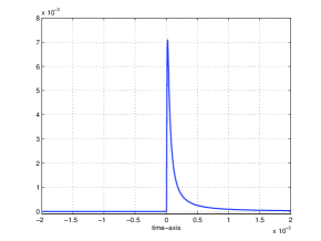
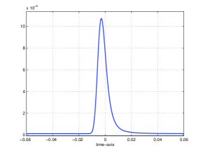
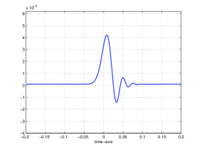
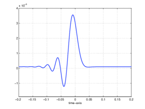
Figure 1: Simulation of $K({\vec{x}},t)$ for the frequency power law with $(\gamma,\alpha_{0})\in\{(0.5,0.1581),\,(1.5,0.0316),\,(2.7,0.0071),\,(3.3,0.0027)\}$, $c_{0}=1$ and $\left|{\vec{x}}\right|=\frac{1}{4}$. In the first example $\gamma<1$ and thus the function is causal. For all other cases it is non causal.

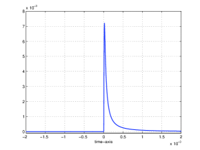
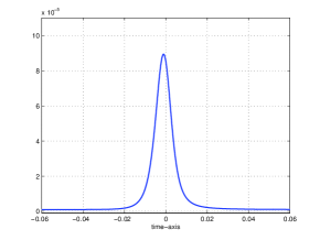
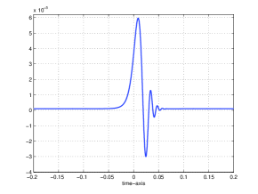
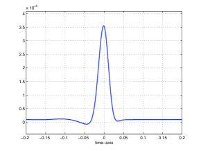
Figure 2: Simulation of $K({\vec{x}},t)$ for Szabo’s frequency law with $(\gamma,\alpha_{0})\in\{(0.5,0.1581),\,(1.5,0.0316),\,(2.7,0.0071),\,(3.3,0.0027)\}$, $c_{0}=1$ and $\left|{\vec{x}}\right|=\frac{1}{4}$.

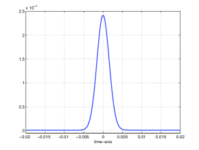
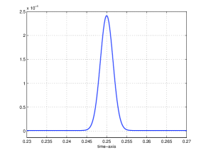
Figure 3: Left: $K({\vec{x}},t)$ defined by the complex thermo-viscous attenuation law with $\tau_{0}=10^{-5}$, $c_{0}=1$ and fixed $\left|{\vec{x}}\right|=\frac{1}{4}$. Right: The proposed law (28) for $\gamma=2$ with $\alpha_{1}=1$, $\tau_{0}=10^{-5}$, $c_{0}=1$ and fixed $\left|{\vec{x}}\right|=\frac{1}{4}$ is causal.

The figures already indicate that power laws with index greater than $1$ violate causality. In the following we support these computational studies by analytical considerations. Thereby we make use of distribution theory, which we recall first. Generally speaking Distributions are generalized functions:

Definition 4

We use the abbreviations:

• $\mathcal{D}:=C_{0}^{\infty}({\mathbb{R}},{\mathbb{C}})$ is the space of infinitely often differentiable functions from ${\mathbb{R}}$ to ${\mathbb{C}}$ which have compact support.

• $\mathcal{S}$ is the space of infinitely often differentiable functions from ${\mathbb{R}}$ to ${\mathbb{C}}$ which are rapidly decreasing. A function $f:{\mathbb{R}}\to{\mathbb{C}}$ is rapidly decreasing if for all $i,j\in{\mathbb{N}}_{0}$

  $$\left|x\right|^{i}\left|f^{(j)}(x)\right|\to 0\text{ for }\left|x\right|\to\infty\;.$$

• $\mathcal{S}$ is a locally convex space (see Y (95) for a definition) with the topology induced by the family of semi-norms

  $$p_{P,j}(f)=\sup_{x\in{\mathbb{R}}}\left|P(x)f^{(j)}(x)\right|,$$

  where $P$ is a polynomial and $j\in{\mathbb{N}}_{0}$. The topology on a locally convex set is defined as follows: $U\subseteq\mathcal{S}$ is open, if for every $f\in U$ there exists $\varepsilon>0$ and a finite non-empty set $J^{\prime}$ of polynomials and a finite set of indices $K^{\prime}$ such that

  $$\bigcap_{P\in J^{\prime},k\in K^{\prime}}\{g\in\mathcal{S}:p_{P,k}(g-f)<\varepsilon\}\subseteq U\;.$$

• The space of tempered distributions, $\mathcal{S}^{\prime}$, is the space of linear continuous functionals and $\mathcal{S}$.

• A functional $L:\mathcal{S}\to{\mathbb{C}}$ is continuous if there exists a constant $C>0$ and a seminorm $p_{P,j}$ such that

  $$\left|Lu\right|\leq Cp_{P,j}(u)\,,\text{ for every }u\in\mathcal{S}$$

  (see (Y, 95, Sect. I.6, Thm. 1)

In the following we give some examples of tempered distributions and review some of their properties. The examples are taken from (Y, 95, Sec6.2, Ex. 3) and (DL02c, , Remark 6).

Example 1

(Examples of Tempered Distributions)

• Let $1\leq p\leq\infty$ and $f\in L^{p}({\mathbb{R}},{\mathbb{C}})$, then the linear operator $T\phi=\int_{{\mathbb{R}}}f(x)\phi(x)\,dx$ is a tempered distribution. In the following we identify $f$ and $T$, and this clarifies the terminology $f\in\mathcal{S}^{\prime}$ later on.

• $\mathcal{S}\subseteq\mathcal{S}^{\prime}$ - thereby already the above relation between functions and tempered distributions is used.

• Distributions with compact support are tempered distributions. For instance the $\delta$-Distribution is a tempered distribution.

• Polynomials are tempered distributions.

• The functions $f$ of $L_{loc}^{1}({\mathbb{R}})$ which are uniformly bounded by a polynomial for $\left|x\right|$ sufficiently large, are tempered distributions.

Lemma 2

• The pointwise limit $f:{\mathbb{R}}\to{\mathbb{C}}$ of a sequence of functions $\{f_{n}:{\mathbb{R}}\to{\mathbb{C}}\}\subseteq\mathcal{S}^{\prime}$, is again a tempered distribution.

• Let $f\in\mathcal{S}^{\prime}$, then $\mathcal{F}\left\{f\right\}\in\mathcal{S}^{\prime}$ and $\mathcal{F}^{-1}\left\{f\right\}\in\mathcal{S}^{\prime}$.

In the following we review Theorem 4 on p294 ff from DL02b which characterized when a generalized function $f\in\mathcal{S}^{\prime}({\mathbb{R}})$ is causal, that is, when $\mbox{supp}(f)\subseteq[0,\infty)$. Below we use the following notation

$${\mathbb{C}}_{\varepsilon}:=\{z\in{\mathbb{C}}:\Im(z)\geq\varepsilon\}\;.$$

Theorem 4.1

(Theorem 4 on p294 ff in DL02b ) Let $f\in\mathcal{S}^{\prime}({\mathbb{R}})$. Then $f$ is causal if and only if

1. There exists a function $F:{\mathbb{C}}_{0}:=\{\xi+{\mathrm{i}}\,\eta:\eta\geq 0\}\to{\mathbb{C}}$, which is holomorphic in the interior $\mathring{{\mathbb{C}}}_{0}:=\{\xi+{\mathrm{i}}\,\eta:\eta>0\}$.

2. For all fixed $\eta>0$ and $\xi\in{\mathbb{R}}$, $F(\xi+{\mathrm{i}}\,\eta)$ is a tempered distribution with respect to the variable $\xi$ and for $\eta\to 0$ $F(\xi+{\mathrm{i}}\,\eta)$ is convergent (with respect to the weak topology on $\mathcal{S}^{\prime}$) to $\mathcal{F}\left\{f\right\}:{\mathbb{R}}\to{\mathbb{C}}$.

3. For every $\varepsilon>0$, there exists a polynomial $P$ such that

   $$\left|F(z)\right|\leq P(\left|z\right|)\qquad\text{for}\qquad z\in{\mathbb{C}}_{\varepsilon}\,.$$

Remark 3

The definition of the Fourier transform in this chapter has a different sign as in DL02b and consequently also ${\mathbb{C}}_{0}$ denotes the upper half plane and not the lower half plane as in DL02b .

For analyzing attenuation laws, we use the following corollary, which is derived from Theorem 4.1.

Corollary 1

Let $\alpha^{*}:{\mathbb{R}}\to{\mathbb{C}}$ be continuous and let there exist a holomorphic extension to ${\mathbb{C}}_{0}$, which for the sake of simplicity of notation is again denoted be $\alpha^{*}$. In addition, let $\alpha^{*}(\xi+{\mathrm{i}}\,\eta)\to\alpha^{*}(\xi)$ for $\eta\to 0$ pointwise. We denote by $\alpha:{\mathbb{C}}_{0}\to{\mathbb{C}}$ the real part of $\alpha^{*}$. Moreover, we assume that there exists a constant $C$ such that

$$\alpha(\omega)\geq C\text{ for all }\omega\in{\mathbb{R}}\;.$$ (37)

1. If in addition

   $$\alpha(z)\geq C\text{ for all }z\in{\mathbb{C}}_{0}\;.$$ (38)

   Then, for every ${\vec{x}}\in{\mathbb{R}}^{3}$, the function

   $$t\to K({\vec{x}},t):=\frac{1}{\sqrt{2\pi}}\mathcal{F}^{-1}\left\{\exp\left(-\alpha^{*}(\cdot)\left|{\vec{x}}\right|\right)\right\}(t)$$ (39)

   is causal.

2. On the other hand, if there exists $C_{1}>0$, $\mu>0$ and $C_{2}\in{\mathbb{R}}$ and a sequence $\{z_{n}\}$ in $\mathring{{\mathbb{C}}}_{0}$ such that

   $$\alpha(z_{n})\leq-C_{1}\left|z_{n}\right|^{\mu}-C_{2}\,,$$ (40)

   then $K$ violates causality.

Proof

Let ${\vec{x}}\in{\mathbb{R}}^{3}$ fixed. We apply Theorem 4.1 to $f(\cdot)=K({\vec{x}},\cdot)$. Therefore, we have

$$\sqrt{2\pi}\mathcal{F}\left\{f\right\}(\omega)=\exp\left(-\alpha^{*}(\omega)\left|{\vec{x}}\right|\right)\;.$$

Under the assumption (37), taking into account that $\alpha_{pl}^{*}$ is continuous, $\mathcal{F}\left\{f\right\}$ is in $L_{loc}^{1}({\mathbb{R}})$ and bounded by a constant polynomial, thus in $\mathcal{S}^{\prime}$ (cf. Example 2), and consequently, according to Lemma 2, $f\in\mathcal{S}^{\prime}$. Therefore, the general assumption of Theorem 4.1 is satisfied.

The function $z\in{\mathbb{C}}_{0}\mapsto F(z):=\exp\left(-\alpha^{*}(z)\left|{\vec{x}}\right|\right)$ is an extension of $2\pi\mathcal{F}\left\{f\right\}(\omega)$, which is holomorphic in $\mathring{{\mathbb{C}}}_{0}$. Thus Item 1 of Theorem 4.1 holds.

• For proving the first assertion, it follows from (38) that for $z=\xi+{\mathrm{i}}\,\eta$ with $\eta\geq 0$,

  $$\left|F(z)\right|\leq\exp\left(-C\left|{\vec{x}}\right|\right)\,,$$ (41)

  which, in particular, shows that for all $\eta\geq 0$, the functions $\xi\to F(\xi+{\mathrm{i}}\,\eta)$ is a tempered distribution (cf. Lemma 2). Hence Item 1 of Theorem 4.1 holds.

  Moreover, since by assumption $\alpha^{*}(\xi+{\mathrm{i}}\,\eta)\to\alpha^{*}(\xi)$ for $\eta\to 0$ pointwise, $F(\xi+{\mathrm{i}}\,\eta)$ converges to $F(\xi)=2\pi\mathcal{F}\left\{f\right\}(\xi)$ pointwise. Because the limit is a tempered distribution and the convergence is with respect to the weak topology $\mathcal{S}^{\prime}$ (cf. Lemma 2). Hence Item 2 of Theorem 4.1 holds.

  Moreover, from (41) it follows that $\left|F(z)\right|$ is bounded by a constant polynomial. Hence Item (3) of Theorem 4.1 holds and therefore Theorem 4.1 guarantees that $t\mapsto K({\vec{x}},t)$ is causal.

• For the second case, Item 3 of Theorem 4.1 is violated. Consequently, $K({\vec{x}},\cdot)$ is not causal.

Power Laws

Theorem 4.2

Let $0<\gamma\in{\mathbb{R}}$, be not an odd number, and $\omega\in{\mathbb{R}}\mapsto\alpha_{pl}^{*}(\omega)=\tilde{\alpha}_{0}(-{\mathrm{i}}\,\omega)^{\gamma}$ be the power law attenuation coefficient from (15), with $\tilde{\alpha}_{0}=\alpha_{0}/\cos\left(\frac{\pi}{2}\gamma\right)$ as in (14). Then, the function $K$, defined in (39), is causal if and only if $\gamma\in(0,1)$.

Proof

Let ${\vec{x}}\in{\mathbb{R}}^{3}$ be fixed. The function $z\in{\mathbb{C}}\mapsto\alpha_{pl}^{*}(z)=\tilde{\alpha}_{0}(-{\mathrm{i}}\,z)^{\gamma}$ is the holomorphic extension of $\omega\in{\mathbb{R}}\mapsto\alpha_{pl}^{*}(\omega)$. We prove or disprove causality by using Corollary 1.

For $z=\left|z\right|\exp\left({\mathrm{i}}\,\phi\right)$ it follows from (15) that

$$\Re((-{\mathrm{i}}\,z)^{\gamma})=\Re(\left|z\right|^{\gamma}\,\exp\left({\mathrm{i}}\,\gamma\,(\phi-\pi/2)\right))=\left|z\right|^{\gamma}\,\cos(\gamma(\phi-\pi/2))\,.$$

This implies that

$$\alpha_{pl}(z)=\tilde{\alpha}_{0}\Re((-{\mathrm{i}}\,z)^{\gamma})=\tilde{\alpha}_{0}\cos(\gamma(\phi-\pi/2))\left|z\right|^{\gamma}\;.$$ (42)

In particular, if $z=\omega\in{\mathbb{R}}$, then $\phi$ is either $0$ or $\pi$. Taking into account the definition of $\tilde{\alpha}_{0}$ and that the $\cos$-function is symmetric around the origin, it follows that

$$\alpha_{pl}(\omega)=\alpha_{0}\left|w\right|^{\gamma}\geq 0\;.$$ (43)

Thus (37) holds.

• Let $\gamma\in(0,1)$: Every $z=\left|z\right|\,\exp\left({\mathrm{i}}\,\phi\right)\in{\mathbb{C}}_{0}$ satisfies $\phi\in[0,\pi]$. Consequently $\gamma(\phi-\pi/2)\in[-\pi/2,\pi/2]$ and thus $\cos(\gamma(\phi-\pi/2))$ is uniformly non-negative. Even more for $\gamma\in(0,1)$ the coefficient $\tilde{\alpha}_{0}$, defined in (14), is positive. In summary, we have that there exists a constant $C_{1}\geq 0$ such that

  $$\alpha_{pl}(z)\geq C_{1}\left|z\right|^{\gamma}\geq 0\qquad\text{ for }\qquad z\in{\mathbb{C}}_{0}\;.$$ (44)

  Thus (38) holds and application of Corollary 1 shows that $K$ is causal.

• Let $\gamma\in(1,3)\cup(5,7)\cup\cdots$. Then $\tilde{\alpha}_{0}<0$. The sequence

  $$\{z_{n}:=n\exp\left({\mathrm{i}}\,\pi/2\right)={\mathrm{i}}\,n\}_{n\in{\mathbb{N}}}$$ (45)

  consists of elements of $\mathring{{\mathbb{C}}}_{0}$ and satisfies assumption (40), that is,

  $$\alpha_{pl}(z_{n})=\underbrace{\tilde{\alpha}_{0}}_{<0}\left|z_{n}\right|^{\gamma}\;.$$ (46)

  Application of Corollary 1 shows that $K$ is not causal.

• Let $\gamma\in(3,5)\cup(7,9)\cup\cdots$. We fix some $0<\delta<\pi/2$, and define

  $$\phi:=\left(1+\frac{1}{\gamma}\right)\frac{\pi}{2}+\frac{\delta}{\gamma}\;.$$

  The sequence

  $$\{z_{n}:=n\,\exp\left({\mathrm{i}}\,\phi\right)\}$$ (47)

  consists of elements of $\mathring{{\mathbb{C}}}_{0}$. Under the above assumptions, it follows that $\tilde{\alpha}_{0}>0$ and therefore

  $$\alpha_{pl}(z_{n})=\underbrace{\tilde{\alpha}_{0}}_{>0}\underbrace{\cos(\pi/2+\delta)}_{<0}\left|z_{n}\right|^{\gamma}\;.$$ (48)

  Thus form Corollary 1 the assertion follows.

In the following we analyze the following family of variants of power laws:

$$\alpha_{pl+}^{*}(\omega)=\tilde{\alpha}_{0}(-{\mathrm{i}}\,\omega)^{\gamma}+\alpha_{1}(-{\mathrm{i}}\,\omega)\,,$$ (49)

which have been considered in S (95); WHBM (00).

Theorem 4.3

Let $0<\gamma\notin{\mathbb{N}}$ and $\alpha_{pl+}^{*}$ as defined in (49). Moreover, let $K$ be as in (39). Then, if $\gamma>1$, $K$ is not causal. For $\gamma\in(0,1)$ $K$ is causal if and only if $\alpha_{1}\in[0,\infty)$.

Proof

The holomorphic extension of $\omega\in{\mathbb{R}}\to\alpha_{pl+}^{*}(\omega)$ is the function

$$\alpha_{pl+}^{*}(z)=\tilde{\alpha}_{0}(-{\mathrm{i}}\,z)^{\gamma}+\alpha_{1}(-{\mathrm{i}}\,z)$$

and consequently

$$\alpha_{pl+}(z)=\tilde{\alpha}_{0}\left|z\right|^{\gamma}\left(1+\frac{\alpha_{1}}{\tilde{\alpha}_{0}}\left|z\right|^{1-\gamma}\right)\cos\left(\gamma\left(\phi-\frac{\pi}{2}\right)\right)\;.$$

• For $\gamma>1$ we have that $1+\frac{\alpha_{1}}{\tilde{\alpha}_{0}}\left|z\right|^{1-\gamma}\to 1$ for $\left|z\right|\to\infty$. Let $\{z_{n}\}$ as defined in (45) or (47). Then, since for both sequences $\left|z_{n}\right|\to\infty$, it follows from (46), (48) that the according sequences $\{z_{n}\}$ satisfy (40) for $n$ sufficiently large, respectively. Thus $K$ is not causal.

• For $\gamma\in(0,1)$ and $\alpha_{1}\geq 0$ the assertion follows already from the fact that $\alpha_{pl+}(\omega)\geq\alpha_{pl}(\omega)$ and that the later already satisfies (38). Thus $K$ is causal.

• Let $\gamma\in(0,1)$ and $\alpha_{1}<0$. Then for some $0<\delta<-\alpha_{1}$ fixed, we can find a constant $C_{2}$ such that for all $z\in{\mathbb{C}}$

  $$\tilde{\alpha}_{0}\left|z\right|^{\gamma}+\alpha_{1}\left|z\right|\leq\underbrace{(\alpha_{1}+\delta)}_{<0}\left|z\right|-C_{2}\;.$$

  Consequently, for $\{z_{n}={\mathrm{i}}\,n\}$, we have

  $$\alpha_{pl+}(z_{n})\leq(\alpha_{1}+\delta)\left|n\right|-C_{2}\;.$$

  which shows (40). Thus $K$ is not causal.

Powerlaw with $\gamma=1$

Theorem 4.4

Let $\alpha_{pl}^{*}$ be as in defined in (17). Then the function $K$, defined in (39) is not causal.

Proof

First, we prove that

$$z\in{\mathbb{C}}_{0}\mapsto\hat{\alpha}_{pl}^{*}(z):=\alpha_{0}z+{\mathrm{i}}\,\frac{2\alpha_{0}}{\pi}z\log\left(\frac{z}{\omega_{0}}\right)$$

is the holomorphic extension of $\omega\to\alpha_{pl}^{*}(\omega)$. This assertion follows from the facts

$$\hat{\alpha}_{pl}^{*}(\omega) =\alpha_{pl}^{*}(\omega)\text{ for } \omega>0\,,$$

$$\lim_{\eta\to 0+}{\mathrm{i}}\,\frac{2}{\pi}\log\left(\frac{\omega+{\mathrm{i}}\,\eta}{\omega_{0}}\right) ={\mathrm{i}}\,\frac{2}{\pi}\,\log\left|\frac{\omega}{\omega_{0}}\right|-2\text{ for } \omega<0\;.$$

Since

$$\alpha_{pl}(\omega)=\Re(\alpha_{pl}^{*}(\omega))=\alpha_{0}\,\left|\omega\right|\geq 0\,,$$

Corollary 1 is applicable. For the elements of the sequence $\{z_{n}:={\mathrm{i}}\,n\}_{n\in{\mathbb{N}}}$ in ${\mathbb{C}}_{0}$

$$\hat{\alpha}_{pl}^{*}(z_{n})=-\frac{2\alpha_{0}}{\pi}n\log\left(\frac{n}{\omega_{0}}\right)$$

is real and therefore equals $\alpha_{pl}(z_{n})$ and thus (40) holds. Thus Corollary 1 gives the assertion.

Szabo’s Model:

Proposition 1

For $\alpha_{0}>0$ let $\alpha_{sz}^{*}$ be the coefficient of Szabo’s model (19). Then, for $\gamma\in(0,1)$, the function $K$ (10) is a causal function and for $\gamma>1$ with $\gamma\not\in{\mathbb{N}}$, $K$ violates causality.

Proof

Without loss of generality we assume that $c_{0}=1$. The holomorphic extension of $\alpha_{sz}^{*}:{\mathbb{R}}\to{\mathbb{C}}$ from (19) is

$$z\in{\mathbb{C}}_{0}\to\alpha_{sz}^{*}(z)=(-{\mathrm{i}}\,z)\left[\sqrt{1+2\tilde{\alpha}_{0}(-{\mathrm{i}}\,z)^{\gamma-1}}-1\right]\,.$$

First, we make some general manipulations which can be used in several ways: Let $z=\xi+{\mathrm{i}}\,\eta\in{\mathbb{C}}_{0}$. We use the polar representation

$$z=\left|z\right|\exp\left({\mathrm{i}}\,\phi\right)\,,\quad\phi:=\phi(z)\in\left[0,\pi\right]\;.$$

Then

$$\alpha_{sz}^{*}(z)=\left|z\right|\exp\left({\mathrm{i}}\,(\phi-\pi/2)\right)\Psi(z)\,,$$

where

$$\Psi(z) :=\sqrt{\hat{\Psi}(z)}-1\,,$$ (50)

$$\hat{\Psi}(z) :=1+2\tilde{\alpha}_{0}\left|z\right|^{\gamma-1}\exp\left({\mathrm{i}}\,\delta\right)\,,$$

$$\delta :=\delta(z):=(\phi-\pi/2)(\gamma-1)\;.$$

With this notation we have

$$\Re(\hat{\Psi}(z)) =1+2\tilde{\alpha}_{0}\cos(\delta)\left|z\right|^{\gamma-1}\,,$$ (51)

$$\Im(\hat{\Psi}(z)) =2\tilde{\alpha}_{0}\sin(\delta)\left|z\right|^{\gamma-1}\,,$$

$$\left|\hat{\Psi}(z)\right| =\left|z\right|^{\gamma-1}\sqrt{(1+2\tilde{\alpha}_{0}\cos(\delta))^{2}+4\tilde{\alpha}_{0}^{2}\sin(\delta)^{2}}\;.$$

Representing $\hat{\Psi}$ in polar coordinates,

$$\hat{\Psi}(z)=\left|\hat{\Psi}(z)\right|\exp\left({\mathrm{i}}\,\theta(z)\right)\,,$$

we get

$$\sqrt{\hat{\Psi}(z)} =\sqrt{\left|\hat{\Psi}(z)\right|}\exp\left({\mathrm{i}}\,\theta(z)/2\right)\qquad\quad\text{ with }$$ (52)

$$\theta(z) =\arctan(\Im(\hat{\Psi}(z))/\Re(\hat{\Psi}(z))))\qquad\theta\in(-\pi,\pi)\;.$$

Note, that $\sqrt{\hat{\Psi}(z)}$ is the complex root with non-negative real part, which meets the general assumption of the paper. Moreover, we have

$$\alpha_{sz}(z)=\Re(\alpha_{sz}^{*}(z))=\eta\Re(\Psi(z))+\xi\Im(\Psi(z))\;.$$ (53)

First, we prove that $\Re(\Psi(z))\geq 0$: We use the elementary inequality

$$\cos(\theta(z))\leq\cos^{2}(\theta(z)/2)\,,$$

and $\cos(\theta(z)/2)\geq 0$ which imply that

$$\Re\left(\sqrt{\hat{\Psi}(z)}\right) =\sqrt{\left|\hat{\Psi}(z)\right|}\cos(\theta(z)/2)$$ (54)

$$=\sqrt{\left|\hat{\Psi}(z)\right|\,\cos^{2}(\theta(z)/2)}$$

$$\geq\sqrt{\Re(\hat{\Psi}(z))}\;.$$

• Now, let $\gamma\in(0,1)$. Since $\Re(\hat{\Psi}(z))\geq 1$ for $\gamma\in(0,1)$, it follows that for all $z\in{\mathbb{C}}_{0}$

  $$\eta\Re(\Psi(z))=\eta\Re\left(\sqrt{\hat{\Psi}(z)}\right)-\eta\geq\eta\sqrt{\Re(\hat{\Psi}(z))}-\eta\geq 0\,.$$

  Thus $\eta\Re(\Psi(z))\geq 0$.

  Now we show that $z\to\xi\Im(\Psi(z))$ is uniformly bounded from below by $0$ in ${\mathbb{C}}_{0}$. Thus according to (53) $\alpha_{sz}$ is uniformly bounded from below, and thus from Corollary 1, it follows that $t\to K({\vec{x}},t)$ is causal.

  Using the definition of $\theta$, (52), and the facts that $\delta\in[0,(1-\gamma)\pi/2]$ for $\phi\in[0,\pi/2]$ and $\delta\in[(\gamma-1)\pi/2,0)$ for $\phi\in(\pi/2,\pi]$ it follows from the monotonicity of $\tan$ on $(-\pi,\pi)$ that

  $$\theta(z)=\arctan\left(\frac{2\tilde{\alpha}_{0}\sin(\delta)\left|z\right|^{\gamma-1}}{1+2\tilde{\alpha}_{0}\cos(\delta)\left|z\right|^{\gamma-1}}\right)\in\left\{\begin{array}[]{rcl}~{}[0,\delta]&\text{ for all }&\phi\in[0,\pi/2]\,,\\ ~{}[\delta,0)&\text{ for all }&\phi\in(\pi/2,\pi]\end{array}\right.$$

  Now, noting that $\mbox{sgn}(\xi)=\mbox{sgn}\left(\sin(\theta(z)/2)\right)$ it follows that

  $$\xi\Im(\Psi(z))=\xi\sqrt{\left|\hat{\Psi}(z)\right|}\sin(\theta(z)/2)\geq 0\,.$$ (55)

  Thus the assertion follows from Corollary 1.

• Assume that $\gamma>1$. Let $z=\xi+{\mathrm{i}}\,\eta$ with $\eta=0$. Since the square root in (50) is such that $\Re(\Psi(z))>0$ for $z\in{\mathbb{C}}_{0}$, property (102) in the Appendix implies $\xi\Im(\Psi(z))>0$ for $z=\xi$ and hence $\alpha_{sz}(z=\xi)\geq 0$. Thus (37) holds and we can apply Corollary 1.

  • Let $\gamma\in(1,3)\cup(5,7)\cup\cdots$, which implies that $\cos\left(\gamma\,\pi/2\right)<0$, and consequently, $\tilde{\alpha}_{0}<0$. For sufficiently large $n$ the elements of the sequence $\{z_{n}:={\mathrm{i}}\,n\}$ satisfy

    $$\alpha_{sz}(z_{n})=n\,\Re\left(\sqrt{1-2\left|\tilde{\alpha}_{0}\right|\,n^{\gamma-1}}-1\right)\leq-n\,,$$

    which shows that (40) holds with $\mu=1$, $C_{1}=1/2$ and $C_{2}=0$, and hence the assertion follows from Corollary 1.

  • Let $\gamma\in(3,5)\cup(7,9)\cup\cdots$, which implies that $\cos\left(\gamma\,\pi/2\right)>0$, and consequently, $\tilde{\alpha}_{0}>0$. Now, let $z_{n}:=n\exp\left({\mathrm{i}}\,\phi\right)$ with

    $$\phi:=\frac{\pi}{\gamma-1}+\frac{\pi}{2}\,.$$

    Since $\gamma>3$, we have $\phi\in(\pi/2,\pi)$, and therefor $\Re(z_{n})=n\,\cos(\phi)<0$ and $\Im(z_{n})=n\,\sin(\phi)>0$. Moreover,

    $$\hat{\Psi}(z_{n})=1-2\,\left|\tilde{\alpha}_{0}\right|\,n^{\gamma-1}\,$$

    and thus for sufficiently large $n$ we have $\Re(\Psi(z_{n}))=-1$ and
    $\Im\left(\sqrt{\hat{\Psi}(z_{n})}\right)\geq C_{1}\,n^{(\gamma-1)/2}$ for some constant $C_{1}>0$. Hence it follows that

    $$\alpha_{sz}(z_{n}) =-\Im(z_{n})+\Re(z_{n})\,\Im(\sqrt{\hat{\Psi}(z_{n})})$$

    $$=-n\left|\sin(\phi)\right|-n\left|\cos(\phi)\right|\,C_{1}\,n^{(\gamma-1)/2}$$

    and therefore (40) holds. Thus from Corollary 1 the assertion follows.

Thermo-Viscous Attenuation Law

Theorem 4.5

Let $c_{0},\tau_{0}>0$ and let $\alpha_{tv}^{*}$ as defined in (20). Then the kernel function $K$ violates causality.

Proof

Since the function $z\in{\mathbb{C}}_{0}\to 1-{\mathrm{i}}\,\tau_{0}\,z$ does not vanish, the function

$$z\in{\mathbb{C}}_{0}\to\alpha_{tv}^{*}(z)=\frac{-{\mathrm{i}}\,z}{c_{0}\,\sqrt{1-{\mathrm{i}}\,\tau_{0}z}}+\frac{{\mathrm{i}}\,z}{c_{0}}$$

is the holomorphic extension of $\omega\in{\mathbb{R}}\to\alpha_{tv}^{*}(\omega)$. That (37) holds follows from the identity (21). For the sequence $\{z_{n}\}_{n\in{\mathbb{N}}}:=\{{\mathrm{i}}\,n\}_{n\in{\mathbb{N}}}$ we get for $n$ sufficiently large

$$\alpha_{tv}^{*}(z_{n})=\frac{n}{c_{0}}\,\left[\frac{1}{\sqrt{1+\tau_{0}\,n}}-1\right]\leq-\frac{1}{2\,c_{0}}n$$

Thus (40) holds.

The second part of Corollary 1 implies that $K$ is not causal.

Model of Nachman, Smith and Waag

Theorem 4.6

Let $\alpha_{nsw}^{*}$ as in (22). If

$$\tilde{\tau}_{m}<\tau_{m}\qquad\mbox{ for all}\qquad m\in\{1,\,\ldots\,,N\}\,,$$ (56)

then the kernel function $K$ is causal.

Proof

Since for all $z\in{\mathbb{C}}_{0}$ and all $1\leq m\leq N$, $1-{\mathrm{i}}\,\tau_{m}\,z$ does not vanish,

$$z\in{\mathbb{C}}_{0}\to\alpha_{nsw}^{*}(z)=\frac{-{\mathrm{i}}\,z}{c_{0}}\,\left[\frac{c_{0}}{\tilde{c}_{0}}\,\sqrt{\frac{1}{N}\,\sum_{m=1}^{N}\frac{1-{\mathrm{i}}\,\,\tilde{\tau}_{m}\,z}{1-{\mathrm{i}}\,\tau_{m}\,z}}-1\right]$$

is the holomorphic extension of $\omega\in{\mathbb{R}}\to\alpha_{nsw}^{*}(\omega)$.

We use a similar notation as in Proposition 1.

$$z=\xi+{\mathrm{i}}\,\eta=\left|z\right|\exp\left({\mathrm{i}}\,\phi\right)\in{\mathbb{C}}_{0}\,,$$

with some $\phi\in[0,\pi]$.

$$\alpha_{nsw}^{*}(z)=\frac{\left|z\right|}{c_{0}}\exp\left({\mathrm{i}}\,(\phi-\pi/2)\right)\,(\Psi(z)-1)\,,$$

where

$$\Psi(z)=\sqrt{\sum_{m=1}^{N}\hat{\Psi}_{m}(z)}\,\quad\mbox{ with }\quad\hat{\Psi}_{m}(z):=\frac{1}{N}\,\frac{c_{0}^{2}}{\tilde{c}_{0}^{2}}\,\frac{1-{\mathrm{i}}\,\,\tilde{\tau}_{m}\,z}{1-{\mathrm{i}}\,\tau_{m}\,z}\,,$$

In the following we show that for all $z\in{\mathbb{C}}_{0}$

$$c_{0}\alpha_{nsw}(z)=\eta(\Re(\Psi)(z)-1)+\xi\Im(\Psi)(z)>0\,,$$ (57)

which means that (38) holds. Then, according to Corollary 1 the function $t\to K({\vec{x}},t)$ is causal.

As in the proof of Proposition 1 we prove $\eta(\Re(\Psi)(z)-1)>0$ and $\xi\Im(\Psi)(z)>0$.

• Taking into account (24) we define

  $$s:=\frac{1}{N}\,\frac{c_{0}^{2}}{\tilde{c}_{0}^{2}}=\left(\sum_{m=1}^{N}\frac{\tilde{\tau}_{m}}{\tau_{m}}\right)^{-1}\,.$$ (58)

  Using this notation, we get

  $$\hat{\Psi}_{m}(z) =s\,\frac{(1+\tilde{\tau}_{m}\,\tau_{m}\,\left|z\right|^{2})+{\mathrm{i}}\,\,(\tau_{m}\,\bar{z}-\tilde{\tau}_{m}\,z)}{|1-{\mathrm{i}}\,\,\tau_{m}\,z|^{2}}$$

  $$=s\,\frac{\tilde{\tau}_{m}}{\tau_{m}}\,\frac{(\tau_{m}/\tilde{\tau}_{m}+\tau_{m}^{2}\,\left|z\right|^{2}+(\tau_{m}^{2}/\tilde{\tau}_{m}+\tau_{m})\,\eta)+{\mathrm{i}}\,\,(\tau_{m}^{2}/\tilde{\tau}_{m}-\tau_{m})\,\xi}{1+\tau_{m}^{2}\,\left|z\right|^{2}+2\,\tau_{m}\,\eta}\,,$$

  Because $\tau_{m}/\tilde{\tau}_{m}>1$, by assumption (56), it follows that for all $z\in{\mathbb{C}}_{0}$

  $$\Re(\hat{\Psi}_{m}(z))>s\,\frac{\tilde{\tau}_{m}}{\tau_{m}}\;.$$

  Consequently, by using the definition of $s$, (58), it follows that

  $$\Re\left(\sum_{m=1}^{N}\hat{\Psi}_{m}(z)\right)>s\,\sum_{m=1}^{N}\frac{\tilde{\tau}_{m}}{\tau_{m}}=1.$$

  Now, using (54) it follows

  $$\Re(\Psi(z))=\Re\left(\sqrt{\sum_{m=1}^{N}\Psi_{m}(z)}\right)\geq\sqrt{\Re\left(\sum_{m=1}^{N}\Psi_{m}(z)\right)}>1$$

  and consequently $\eta(\Re(\Psi(z))-1)>0$.

• We have

  $$\Im(\hat{\Psi}_{m}(z))=s\,\frac{\tilde{\tau}_{m}}{\tau_{m}}\,\frac{(\tau_{m}^{2}/\tilde{\tau}_{m}-\tau_{m})\,\xi}{1+\tau_{m}^{2}\,\left|z\right|^{2}+2\,\tau_{m}\,\eta}$$

  together with the assumption (56), which state that $\tau_{m}/\tilde{\tau}_{m}>1$, it follows that $\mbox{sgn}(\Im(\hat{\Psi}_{m}(z)))=\mbox{sgn}(\xi)$. According to our assumption, we take that complex root, such that the real part of the argument is non-negative which together with property (102) in the Appendix implies

  $$\mbox{sgn}\left(\Im\left(\sqrt{\sum_{m=1}^{N}\hat{\Psi}_{m}(z)}\right)\right)=\mbox{sgn}\left(\Im\left(\sum_{m=1}^{N}\hat{\Psi}_{m}(z)\right)\right)\,.$$

  Therefore,

  $$\mbox{sgn}(\Im(\Psi(z))) =\mbox{sgn}\left(\Im\left(\sqrt{\sum_{m=1}^{N}\hat{\Psi}_{m}(z)}\}\right)\right)$$

  $$=\mbox{sgn}\left(\Im\left(\sum_{m=1}^{N}\hat{\Psi}_{m}(z)\right)\right)=\mbox{sgn}(\xi)\;.$$

  This shows the assertion.

Our Model

Theorem 4.7

For $\alpha_{0},\,\tau_{0}>0$ and $\gamma\in(1,2]$ let $\alpha_{ksb}^{*}$ be defined as in (28). Then $K$, as defined in (39), is causal.

Proof

The function $\hat{z}\to 1+(-{\mathrm{i}}\,\tau_{0}\hat{z})$ does not vanish in ${\mathbb{C}}_{0}$. Thus the holomorphic extension of $\omega\to\alpha_{ksb}^{*}(\omega)$ is given by

$$\hat{z}\in{\mathbb{C}}_{0}\to\alpha_{ksb}^{*}(\hat{z})=\frac{\alpha_{0}(-{\mathrm{i}}\,\hat{z})}{c_{0}\sqrt{1+(-{\mathrm{i}}\,\tau_{0}\hat{z})^{\gamma-1}}}\;.$$

In the following let $\hat{z}\in{\mathbb{C}}_{0}$. For proving (38) we make a variable transformation

$$\alpha_{ksb}^{*}(\hat{z})=\frac{-{\mathrm{i}}\,\tau_{0}\hat{z}}{\sqrt{1+(-{\mathrm{i}}\,\tau_{0}\hat{z})^{\gamma-1}}}=\frac{\alpha_{0}}{\tau_{0}c_{0}}\frac{-{\mathrm{i}}\,z}{\sqrt{1+(-{\mathrm{i}}\,z^{\gamma-1})}}\,,$$

and define

$$\Psi(z)=\frac{1}{\sqrt{\hat{\Psi}(z)}}\quad\text{ and }\quad\hat{\Psi}(z)=1+(-{\mathrm{i}}\,\,z)^{\gamma-1}\;.$$

Then, with this notation, in order to prove causality of $K$, it suffices to prove that for all $z\in{\mathbb{C}}_{0}$

$$\frac{\tau_{0}c_{0}}{\alpha_{0}}\alpha_{ksb}(\hat{z})=\eta\Re(\Psi(z))+\xi\Im(\Psi(z))\geq 0\;.$$ (59)

As in the proof of Proposition 1 we show that both terms $\eta\Re(\Psi(z))$ and $\xi\Im(\Psi(z))$ are non-negative, and then from Corollary 1 the assertion follows.

In order to prove (59) we note that the function $\hat{\Psi}$ here is the same as in (50) in the proof of Proposition 1 when $\tilde{\alpha}_{0}$ is set to $1/2$. Thus we can already rely on the series of manipulations for $\hat{\Psi}$ developed in the proof of Proposition 1.

• Since $\eta\geq 0$ it suffices to show that $\Re(\Psi(z))\geq 0$. We note that for a complex number $a+{\mathrm{i}}\,b$

  $$\Re\left(\frac{1}{a+{\mathrm{i}}\,b}\right)=\Re\left(\frac{a-{\mathrm{i}}\,b}{a^{2}+b^{2}}\right)=\frac{1}{a^{2}+b^{2}}\Re(a+{\mathrm{i}}\,b)\;.$$

  Taking into account the definition of $\Psi$ it therefore suffices to show that $\Re\left(\sqrt{\hat{\Psi}(z)}\right)\geq 0$ in ${\mathbb{C}}_{0}$. Since $\Re\left(\hat{\Psi}(z)\right)\geq 0$ in ${\mathbb{C}}_{0}$ for $\gamma\in(1,2]$, it follows that $\Re\left(\sqrt{\hat{\Psi}(z)}\right)\geq 0$ in ${\mathbb{C}}_{0}$.

• Now, using that

  $$\Im\left(\frac{1}{a+{\mathrm{i}}\,b}\right)=\Im\left(\frac{a-{\mathrm{i}}\,b}{a^{2}+b^{2}}\right)=-\frac{1}{a^{2}+b^{2}}\Im(a+{\mathrm{i}}\,b)\,,$$

  it suffices to show that $-\xi\Im(\sqrt{\hat{\Psi}(z)})\geq 0$ for proving that $\xi\Im(\Psi(z))\geq 0$. The proof is along the lines as the analogous part in Proposition 1 by taking into account that here $\gamma\in(1,2)$ (in Proposition 1 $\gamma\in(0,1)$). In this case we have now that sign of $\delta$ is exactly opposite as in the proof of Proposition 1, which in turn gives that $\Im(\Psi(z))$ has the opposite sign as well, and consequently $-\xi\Im(\sqrt{\hat{\Psi}(z)})\geq 0$. Thus the assertion follows from Corollary 1.

In experiments it has been discovered that several biological tissues satisfy a frequency power law (16) with exponent $\gamma\in(1,2)$ (cf. W (00); BRBP (010)). However, as it has been shown in Theorem 4.2, such models are not causal. Our proposed model approximates the frequency power law for small frequencies, which is actually the range where it has been experimentally validated. So, our proposed model, is valid in the actual range of experimentally measured data and extrapolates the measured data in a causal way. Figure 4 shows a comparison of $\alpha_{pl}$ and $\alpha_{ksb}$ in an experimental frequency range.

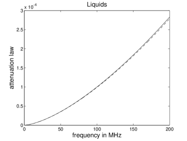
Figure 4: For $\gamma=1.5$: Comparison $\omega\to\alpha_{ksb}(\omega)$ (as defined in (28)) where $\alpha_{0}:=2c_{0}\tau_{0}/\left|\cos(\frac{\pi}{2}\gamma)\right|$ (dashed line) and the power law $\alpha_{pl}(\omega)=\left|\tau_{0}\,\omega\right|^{\gamma}$ (as defined in (16)). For liquids: $\tau_{0}=10^{-6}\,MHz$ (left picture) and for gases: $\tau_{0}=10^{-4}\,MHz$ (right picture) (cf. KFCS (00)). Experiments for determining the power law coefficient are performed in the range $0-60\,MHz$ (cf. e.g. S (95)), which is the basis for the range of the represented data.

Model of Greenleaf and Patch

Proposition 2

For $\alpha_{0}>0$ let $\alpha_{gp}^{*}$ be defined as in (25) with the specified values $\gamma\in\{1,2\}$. Then $K$, as defined in (39), is not causal.

Proof

For the two specified models we have $\alpha_{gp1}(\omega)=a_{0}\left|\omega\right|>0$ and $\alpha_{gp2}(\omega)=a_{0}\omega^{2}$. The respective holomorphic extensions are given by (cf. Proof of Theorem 4.4 and Theorem 4.2)

$$z\in{\mathbb{C}}_{0}\mapsto\hat{\alpha}_{gp1}^{*}(z):=a_{0}z+{\mathrm{i}}\,\frac{2a_{0}}{\pi}z\log\left(\frac{z}{\omega_{0}}\right)\qquad(\omega_{0}\neq 0,\mbox{fixed})$$

and

$$z\in{\mathbb{C}}_{0}\mapsto\hat{\alpha}_{gp2}^{*}(z):=a_{0}\,(-{\mathrm{i}}\,\,z)^{2}\,.$$

The assertion for $\gamma=1$ follows as in the proof of Theorem 4.4 and the second assertion follows from Theorem 4.2 for $\gamma=2$.

Model of Chen and Holm

Theorem 4.8

Let $0<\alpha_{1}<1$, $\gamma\in(0,2)$ and $\mathcal{G}$ as in (26). Then there does not exist a constant $c>0$ such that

$$\mbox{supp}(\mathcal{G}\left(\cdot,t\right))\subseteq B_{c\,t}({\mathbf{0}})\qquad\mbox{ for }\qquad t>0\,,$$ (60)

i.e. for each $c>0$ the function $t\mapsto\mathcal{G}({\vec{x}},t+\left|{\vec{x}}\right|/c)$ is not causal.

Proof

Let $t>0$ be fixed. Assume that ${\vec{x}}\mapsto\mathcal{G}({\vec{x}},t)$ has support in $B_{c\,t}({\mathbf{0}})$ for some $c>0$. Then according to the Paley-Wiener-Schwartz Theorem (Cf. GW (99); H (03)) the map $\mathbf{k}\mapsto\mathcal{F}^{-1}\left\{\mathcal{G}\right\}(\mathbf{k},t)$ is infinitely differentiable. We show that this is not possible. According to (26) and (27), we have

$$\mathcal{F}_{3D}^{-1}\left\{\mathcal{G}\right\}(\mathbf{k},t)=\frac{H(t)\,c_{0}^{2}}{(2\,\pi)^{3/2}}\,\exp\left(A(\mathbf{k})\,t\right)\,\frac{\sin(B(\mathbf{k})\,t)}{B(\mathbf{k})}$$

with

$$A(\mathbf{k}):=-\alpha_{1}\,c_{0}\,\left|\mathbf{k}\right|^{\gamma}\,,\qquad B(\mathbf{k}):=c_{0}\,\sqrt{\left|\mathbf{k}\right|^{2}-\alpha_{1}^{2}\,\left|\mathbf{k}\right|^{2\,\gamma}}\,.$$

Since $\gamma\in(0,2)$, the function $\mathbf{k}\mapsto\exp\left(A(\mathbf{k})\,t\right)$ is not infinitely often differentiable at $\mathbf{k}={\mathbf{0}}$ and since the holomorphic function $\frac{\sin(B(\mathbf{k})\,t)}{B(\mathbf{k})}$ does not vanish at $\mathbf{k}={\mathbf{0}}$, it follows that $\mathbf{k}\mapsto\mathcal{F}_{3D}^{-1}\{\mathcal{G}\}(\mathbf{k},t)$ is not infinitely often differentiable at $\mathbf{k}={\mathbf{0}}$. Consequently, ${\vec{x}}\mapsto\mathcal{G}({\vec{x}},t)$ cannot have compact support, which concludes the proof.

5 Integro-Differential Equations Describing Attenuation

In the following we derive the integro-differential equations for the attenuated pressure $p_{\text{att}}$ for various attenuation laws. Thereby, we first derive equations which the according attenuated Green functions $\mathcal{G}$ (cf. (9)) are satisfying, and then, by convolution, we derive the equations for $p_{\text{att}}$. The integro-differential equations are general in the sense, that they apply to arbitrary source terms $f$, and in particular to the source term $f$ (6) of the forward problem of photoacoustic imaging with attenuated waves.

For this purpose, we rewrite $\nabla^{2}\mathcal{F}\left\{\mathcal{G}\right\}$ by using its definition (9), i.e. $\mathcal{G}=K*_{t}\mathcal{G}_{0}$, and the product differentiation rule, which gives

$$\frac{1}{\sqrt{2\,\pi}}\,\nabla^{2}\mathcal{F}\left\{\mathcal{G}\right\}$$ (61)

$$= \nabla^{2}\mathcal{F}\left\{K\right\}\cdot\mathcal{F}\left\{\mathcal{G}_{0}\right\}+2\nabla\mathcal{F}\left\{K\right\}\cdot\nabla\mathcal{F}\left\{\mathcal{G}_{0}\right\}+\mathcal{F}\left\{K\right\}\cdot\nabla^{2}\mathcal{F}\left\{\mathcal{G}_{0}\right\}.$$

To evaluate the expression on the right hand side, we calculate $\nabla\mathcal{F}\left\{K\right\}$ and $\nabla^{2}\mathcal{F}\left\{K\right\}$. From (10), it follows that

$$\nabla\mathcal{F}\left\{K\right\}=-\beta^{*}{}^{\prime}\cdot\mathcal{F}\left\{K\right\}\cdot\mbox{sgn}\,,$$ (62)

where $\beta^{*}{}^{\prime}$ denotes the derivative of $\beta^{*}(r,\omega)$ (cf. (10)) with respect to $r$. This together with the formula (103) in the Appendix implies that

$$\nabla^{2}\mathcal{F}\left\{K\right\}$$ (63)

$$= -\nabla\cdot\left(\beta^{*}{}^{\prime}\cdot\mathcal{F}\left\{K\right\}\cdot\mbox{sgn}\right)$$

$$= -(\nabla\cdot\mbox{sgn})\cdot\beta^{*}{}^{\prime}\cdot\mathcal{F}\left\{K\right\}-(\mbox{sgn}\cdot\nabla\beta^{*}{}^{\prime})\cdot\mathcal{F}\left\{K\right\}-(\mbox{sgn}\cdot\nabla\mathcal{F}\left\{K\right\})\cdot\beta^{*}{}^{\prime}$$

$$= \left[-\frac{2}{\left|{\vec{x}}\right|}\cdot\beta^{*}{}^{\prime}-\beta^{*}{}^{\prime\prime}+\left(\beta^{*}{}^{\prime}\right)^{2}\right]\cdot\mathcal{F}\left\{K\right\}.$$

Inserting (62) and (63) into (61) and using again the identity $\mathcal{G}=K*_{t}\mathcal{G}_{0}$, shows that

$$\frac{1}{\sqrt{2\,\pi}}\,\nabla^{2}\mathcal{F}\left\{\mathcal{G}\right\}$$ (64)

$$\qquad=\frac{1}{\sqrt{2\,\pi}}\,\left[-\frac{2}{\left|{\vec{x}}\right|}\cdot\beta^{*}{}^{\prime}-\beta^{*}{}^{\prime\prime}+\left(\beta^{*}{}^{\prime}\right)^{2}\right]\cdot\mathcal{F}\left\{\mathcal{G}\right\}$$

$$\qquad\quad-2\beta^{*}{}^{\prime}\cdot\mathcal{F}\left\{K\right\}\cdot(\mbox{sgn}\cdot\nabla\mathcal{F}\left\{\mathcal{G}_{0}\right\})+\mathcal{F}\left\{K\right\}\cdot\nabla^{2}\mathcal{F}\left\{\mathcal{G}_{0}\right\}.$$

From this identity, together with the two following properties of $\mathcal{G}_{0}$,

$$\nabla\mathcal{F}\left\{\mathcal{G}_{0}\right\}=\left[\frac{{\mathrm{i}}\,\omega}{c_{0}}-\frac{1}{\left|{\vec{x}}\right|}\right]\cdot\mathcal{F}\left\{\mathcal{G}_{0}\right\}\cdot\mbox{sgn}\,,$$ (65)

and

$$\nabla^{2}\mathcal{F}\left\{\mathcal{G}_{0}\right\}+\frac{\omega^{2}}{c_{0}^{2}}\mathcal{F}\left\{\mathcal{G}_{0}\right\}=-\frac{1}{\sqrt{2\pi}}\delta_{\vec{x}}\,,$$ (66)

it follows that

$$\nabla^{2}\mathcal{F}\left\{\mathcal{G}\right\}= \left[-\frac{2}{\left|{\vec{x}}\right|}\cdot\beta^{*}{}^{\prime}-\beta^{*}{}^{\prime\prime}+\left(\beta^{*}{}^{\prime}\right)^{2}\right]\cdot\mathcal{F}\left\{\mathcal{G}\right\}$$ (67)

$$-2\left[\frac{{\mathrm{i}}\,\omega}{c_{0}}-\frac{1}{\left|{\vec{x}}\right|}\right]\cdot\beta^{*}{}^{\prime}\cdot\mathcal{F}\left\{\mathcal{G}\right\}$$

$$-\frac{\omega^{2}}{c_{0}^{2}}\cdot\mathcal{F}\left\{\mathcal{G}\right\}$$

$$-\mathcal{F}\left\{K\right\}\cdot\delta_{\vec{x}}\;.$$

Inserting the identity $\mathcal{F}\left\{K\right\}({\vec{x}},\omega)\cdot\delta_{\vec{x}}=\mathcal{F}\left\{K\right\}({\bf 0},\omega)\cdot\delta_{\vec{x}}$ in (67) gives the Helmholtz equation

$$\nabla^{2}\mathcal{F}\left\{\mathcal{G}\right\}-\left[\beta^{*}{}^{\prime}+\frac{(-{\mathrm{i}}\,\,\omega)}{c_{0}}\right]^{2}\cdot\mathcal{F}\left\{\mathcal{G}\right\}$$ (68)

$$= -\beta^{*}{}^{\prime\prime}\cdot\mathcal{F}\left\{\mathcal{G}\right\}-\mathcal{F}\left\{K\right\}({\bf 0},\cdot)\cdot\delta_{\vec{x}}$$

$$= -\beta^{*}{}^{\prime\prime}\cdot\mathcal{F}\left\{\mathcal{G}\right\}-\frac{1}{\sqrt{2\pi}}\exp\left(-\beta^{*}({\bf 0},\omega)\right)\cdot\delta_{\vec{x}}\,.$$

To reformulate (68) in space–time coordinates, we introduce two convolution operators:

$$D_{*}f:=K_{*}*_{t}f\qquad\text{and}\qquad D_{*}^{\prime}f:=K_{*}^{\prime}*_{t}f,$$ (69)

where the kernels $K_{*}$ and $K_{*}^{\prime}$ are given by

$$K_{*}:=K_{*}({\vec{x}},t):=K_{*}(\left|{\vec{x}}\right|,t)\quad\text{and}\quad K_{*}(r,t):=\frac{1}{\sqrt{2\pi}}\mathcal{F}^{-1}\left\{\beta^{*}{}^{\prime}\right\}(r,t)$$ (70)

and

$$K_{*}^{\prime}:=K_{*}^{\prime}({\vec{x}},t):=K_{*}^{\prime}(\left|{\vec{x}}\right|,t)\quad\text{and}\quad K_{*}^{\prime}(r,t)=\frac{1}{\sqrt{2\pi}}\mathcal{F}^{-1}\left\{\beta^{*}{}^{\prime\prime}\right\}(r,t).$$ (71)

Using these operators and applying the inverse Fourier transform to (68) gives

$$\nabla^{2}\mathcal{G}-\left[D_{*}+\frac{1}{c_{0}}\frac{\partial}{\partial t}\right]^{2}\mathcal{G}=-D_{*}^{\prime}\mathcal{G}-K({\bf 0},\cdot)\delta_{\vec{x}}\;.$$ (72)

In the case that $\beta^{*}(\left|{\vec{x}}\right|,\omega)=\alpha^{*}(\omega)\left|{\vec{x}}\right|$ is of standard form (13), it follows that

$$K_{*}(t)=\frac{1}{\sqrt{2\pi}}\mathcal{F}^{-1}\left\{\alpha^{*}\right\}(t)\qquad\text{ and }\qquad K_{*}^{\prime}\equiv 0\;.$$ (73)

For a general source term $f$, we denote the attenuated wave by $p_{\text{att}}$. That is

$$p_{\text{att}}:=p_{\text{att}}({\vec{x}},t)=\mathcal{G}*_{{\vec{x}},t}f=:\mathcal{A}f\,,$$

where $\mathcal{A}$ is the convolution operator according to the Green function $\mathcal{G}$. This then shows that $p_{\text{att}}$ satisfies the integro-differential equation

$$\boxed{\nabla^{2}p_{\text{att}}-\frac{1}{c_{0}^{2}}\frac{\partial^{2}p_{\text{att}}}{\partial t^{2}}=-\mathcal{A}_{s}f\;,}$$ (74)

where $\mathcal{A}_{s}$ denotes the space–time convolution operator with kernel

$$K_{s}:=K_{s}({\vec{x}},t):=-(\mathcal{B}\mathcal{G})({\vec{x}},t)+(D_{*}^{\prime}\mathcal{G})({\vec{x}},t)+K({\bf 0},t)\cdot\delta_{\vec{x}}({\vec{x}})$$ (75)

and

$$\mathcal{B}:=D_{*}^{2}+\frac{2}{c_{0}}D_{*}\frac{\partial}{\partial t}\;.$$ (76)

Equation (74) is called pressure wave equation with attenuation coefficient $\beta^{*}$. We emphasize that $\beta^{*}$ determines the operators $D_{*}$ and $D^{\prime}_{*}$ which in turn determine the operator $\mathcal{A}_{s}$, which in turn determines $p_{\text{att}}$ - this reveals the dependence of $p_{\text{att}}$ from $\beta_{*}$.

Remark 4

Let $\beta^{*}(r,\omega)=\alpha^{*}(\omega)r$ be the standard attenuation model (cf. (12)). Assuming that the associated kernel $K$ (cf. (39)) is causal, it follows that

$$\left|\nabla K\right|=\frac{1}{\sqrt{2\pi}}\left|\mathcal{F}^{-1}\left\{\alpha^{*}\cdot\exp\left(-\alpha^{*}\left|{\vec{x}}\right|\right)\right\}\right|\;.$$

Using some sequence $\{{\vec{x}}_{n}\}$ satisfying ${\vec{x}}_{n}\neq{\bf 0}$ and ${\vec{x}}_{n}\to{\bf 0}$ shows that

$$\lim_{n\to\infty}\left|\nabla K\right|({\vec{x}}_{n},t)=\frac{1}{\sqrt{2\pi}}\left|\mathcal{F}^{-1}\left\{\alpha^{*}\right\}(t)\right|\underbrace{=}_{(\ref{eq:defKK'+})}\left|K_{*}(t)\right|\;.$$

Due to the causality of $K$ the left hand side is zero for $t<0$, and thus $K_{*}$ is also causal.

Because the convolution of causal distributions is well-defined, the operator $D_{*}$ is well-defined on all causal distributions. Moreover, since $K_{*}^{\prime}=0$, it follows that $D_{*}^{\prime}\equiv 0$. Using that $K_{*}$ depends only on $t$ it follows that

$$(D_{*}\mathcal{G})*_{{\vec{x}},t}f=[K_{*}*_{t}\mathcal{G}]*_{{\vec{x}},t}f=K_{*}*_{t}[\mathcal{G}*_{{\vec{x}},t}f]=D_{*}(\mathcal{G}*_{{\vec{x}},t}f).$$

Convolving each term in (72) with a function $f$, using the previous identity and that $D_{*}^{\prime}\equiv 0$, it follows that

$$\nabla^{2}p_{\text{att}}-\left[D_{*}+\frac{1}{c_{0}}\frac{\partial}{\partial t}\right]^{2}p_{\text{att}}=-f\;$$ (77)

where

$$D_{*}\cdot=\frac{1}{\sqrt{2\,\pi}}\,\mathcal{F}\left\{\alpha^{*}\right\}(t)*_{t}\cdot\,.$$ (78)

In the following we derive the common forms of the wave equation models corresponding to the various attenuation models listed in Section 2.

Power Laws

• Let $0<\gamma\not\in{\mathbb{N}}$ and $0<\alpha_{0}$. We note that the Riemann-Liouville fractional derivative with respect to time, denote by $D_{t}^{\gamma}$ (see KST (06); P (99)), is defined in the Fourier domain by

  $$\mathcal{F}\left\{D_{t}^{\gamma}f\right\}=(-{\mathrm{i}}\,\omega)^{\gamma}\mathcal{F}\left\{f\right\}\,,$$ (79)

  and satisfies

  $$D_{t}^{2\gamma}f=D_{t}^{\gamma}D_{t}^{\gamma}f\qquad\text{and}\qquad\frac{\partial}{\partial t}D_{t}^{\gamma}f=D_{t}^{\gamma}\frac{\partial}{\partial t}f=D_{t}^{\gamma+1}f.$$ (80)

  From this together with (15) and (78), we infer

  $$D_{*}=\tilde{\alpha}_{0}\,D_{t}^{\gamma}\qquad\mbox{ with }\qquad\tilde{\alpha}_{0}:=\frac{\alpha_{0}}{\cos(\pi\,\gamma/2)}$$ (81)

  and thus wave equation (77) reads as follows

  $$\boxed{\begin{aligned} \nabla^{2}p_{\text{att}}&-\left[\tilde{\alpha}_{0}\,D_{t}^{\gamma}+\frac{1}{c_{0}}\frac{\partial}{\partial t}\right]^{2}p_{\text{att}}=-f\;.\end{aligned}}$$ (82)

• Let $\gamma=1$, then for the frequency power law (17) it follows from the Fourier transform table I in L (64)

  $$D_{*} =-\frac{4\,\alpha_{0}}{2\,\pi}\left[\,\frac{H(t)}{t^{2}}-(\log|\omega_{0}|)\,\delta^{\prime}_{t}\right]*_{t}$$

  $$=-\frac{4\,\alpha_{0}}{2\,\pi}\,\frac{H(t)}{t^{2}}*_{t}\;\;+\frac{4\,\alpha_{0}}{\sqrt{2\,\pi}}\,(\log|\omega_{0}|)\,\frac{\partial}{\partial t}\,.$$

Szabo’s Attenuation Law:

Let $0<\alpha_{0}$ and $0<\gamma\not\in{\mathbb{N}}$. From (19) and (79), we get

$$\left[D_{*}+\frac{1}{c_{0}}\frac{\partial}{\partial t}\right]^{2}=\frac{1}{c_{0}^{2}}\frac{\partial^{2}}{\partial t^{2}}+\frac{2\,\tilde{\alpha}_{0}}{c_{0}}\,\frac{\partial}{\partial t}\,D_{t}^{\gamma}$$

and thus wave equation (77) reads as follows

$$\boxed{\nabla^{2}p_{\text{att}}-\frac{1}{c_{0}^{2}}\frac{\partial^{2}p_{\text{att}}}{\partial t^{2}}-\frac{2\,\tilde{\alpha}_{0}}{c_{0}}\,\frac{\partial}{\partial t}\,D_{t}^{\gamma}p_{\text{att}}=-f({\vec{x}},t)\,.}$$ (83)

Thermo-Viscous Attenuation Law:

From (20) we get

$$\left(\mbox{Id}+\tau_{0}\,\frac{\partial}{\partial t}\right)\,\left[D_{*}+\frac{1}{c_{0}}\frac{\partial}{\partial t}\right]^{2}=\frac{1}{c_{0}^{2}}\frac{\partial^{2}}{\partial t^{2}}$$

and thus (77) becomes

$$\boxed{\left(\mbox{Id}+\tau_{0}\,\frac{\partial}{\partial t}\right)\,\nabla^{2}p_{\text{att}}-\frac{1}{c_{0}^{2}}\frac{\partial^{2}p_{\text{att}}}{\partial t^{2}}=-\left(\mbox{Id}+\tau_{0}\,\frac{\partial}{\partial t}\right)\,f\,.}$$ (84)

This equation is called the thermo-viscous wave equation.

Nachman, Smith and Waag NSW (90):

We carry out the details only for one relaxation process.

• $N=1$: From (22) we get

  $$\left(\alpha^{*}(\omega)+\frac{(-{\mathrm{i}}\,\,\omega)}{c_{0}}\right)^{2}=\frac{(-{\mathrm{i}}\,\,\omega)^{2}}{\tilde{c}_{0}^{2}}\,\frac{1-{\mathrm{i}}\,\,\tilde{\tau}_{1}\,\omega}{1-{\mathrm{i}}\,\,\tau_{1}\,\omega}$$

  which implies

  $$\left(\mbox{Id}+\tau_{1}\,\frac{\partial}{\partial t}\right)\,\left[D_{*}+\frac{1}{c_{0}}\frac{\partial}{\partial t}\right]^{2}=\left(\mbox{Id}+\tilde{\tau}_{1}\,\frac{\partial}{\partial t}\right)\,\frac{1}{\tilde{c}_{0}^{2}}\frac{\partial^{2}}{\partial t^{2}}\,.$$

  Thus (77) reads as follows

  $$\boxed{\begin{aligned} \left(\mbox{Id}+\tau_{1}\,\frac{\partial}{\partial t}\right)\,\nabla^{2}p_{\text{att}}&-\frac{1}{\tilde{c}_{0}^{2}}\left(\mbox{Id}+\tilde{\tau}_{1}\,\frac{\partial}{\partial t}\right)\,\frac{\partial^{2}p_{\text{att}}}{\partial t^{2}}\\ &=-\left(\mbox{Id}+\tau_{1}\,\frac{\partial}{\partial t}\right)\,f\,.\end{aligned}}$$ (85)

  If the term with $\tilde{\tau}_{1}=0$ is dropped and $\tilde{c}_{0}$ is replaced by $c_{0}$, then we obtain the thermo-viscous wave equation (84).

• $N>1$: For the general case we refer to equation (26) in NSW (90).

Greenleaf and Patch PG (06):

• For $\gamma=2$ the attenuation coefficient equals to

  $$\alpha^{*}(\omega)=\alpha_{0}\,\omega^{2}=\tilde{\alpha}_{0}\,(-{\mathrm{i}}\,\omega)^{2}\,,$$

  where $\tilde{\alpha}_{0}$ is defined as in (81) and thus

  $$D_{*}=-\alpha_{0}\,\frac{\partial^{2}}{\partial t^{2}}=-\alpha_{0}\,D_{t}^{2}\,,$$

  which gives wave equation (82) with $\gamma=2$.

• For $\gamma=1$ we have

  $$\alpha^{*}(\omega)=\alpha_{0}\,|\omega|=\alpha_{0}\,(-{\mathrm{i}}\,\omega)\,{\mathrm{i}}\,\mbox{sgn}(\omega)$$

  and thus

  $$D_{*}=\alpha_{0}\,\mathbf{D}^{-1}=-\alpha_{0}\,\frac{\partial}{\partial t}\mathcal{H}\,,$$

  where $\mathbf{D}^{-1}$ and $\mathcal{H}$ denote the Riesz fractional differentiation operator and the Hilbert transform (cf. Appendix), respectively. Therefore the wave equation reads as follows

  $$\boxed{\begin{aligned} \nabla^{2}p_{\text{att}}&-\left[\alpha_{0}\,\mathbf{D}^{-1}+\frac{1}{c_{0}}\frac{\partial}{\partial t}\right]^{2}p_{\text{att}}=-f\;.\end{aligned}}$$

Chen and Holm CH (04):

Let $\gamma\in(0,2)$. The Green function defined by (26) satisfies the Helmholtz equation

$$\frac{\partial^{2}\mathcal{F}\left\{\mathcal{G}\right\}}{\partial t^{2}}(\mathbf{k},t)+2\,\alpha_{1}\,c_{0}\,\left|\mathbf{k}\right|^{\gamma}\,\frac{\partial\mathcal{F}\left\{\mathcal{G}\right\}}{\partial t}(\mathbf{k},t)+c_{0}^{2}\,\left|\mathbf{k}\right|^{2}\,\mathcal{F}\left\{\mathcal{G}\right\}(\mathbf{k},t)$$ (86)

$$= \frac{c_{0}^{2}}{(2\,\pi)^{3/2}}\,\delta(t)$$

for $t\in{\mathbb{R}}$ and $\mathbf{k}\in{\mathbb{R}}^{3}$. Since the fractional Laplacian for a rotational symmetric function $f$ and $\gamma\in(0,2)$ is defined by (cf. Definition (2.10.1) in (KST (06))

$$\left(-\nabla^{2}\right)^{\gamma/2}f({\vec{x}})$$

$$:= \frac{1}{\sqrt{(2\,\pi)^{3}}}\,\int_{{\mathbb{R}}^{3}}\exp\left({\vec{x}}\cdot\mathbf{k}\right)\,\left[\left|\mathbf{k}\right|^{\gamma}\,\frac{1}{\sqrt{(2\,\pi)^{3}}}\,\int_{{\mathbb{R}}^{3}}\exp\left(-{\vec{x}}\cdot\mathbf{k}\right)\,f({\vec{x}})\,\mbox{d}{\vec{x}}\right]\,\mbox{d}\mathbf{k}$$

$$= \mathcal{F}_{3D}\left\{\left|\mathbf{k}\right|^{\gamma}\,\mathcal{F}_{3D}^{-1}\{f\}(\mathbf{k})\right\}({\vec{x}})\,,$$

we obtain the following wave equation for $p_{\text{att}}:=\mathcal{G}\ast_{{\vec{x}},t}f$

$$\boxed{\begin{aligned} \nabla^{2}p_{\text{att}}-\frac{1}{c_{0}^{2}}\frac{\partial^{2}p_{\text{att}}}{\partial t^{2}}-\frac{2\,\alpha_{1}}{c_{0}}\,\frac{\partial}{\partial t}\,\left(-\nabla^{2}\right)^{\gamma/2}p_{\text{att}}=-f({\vec{x}},t)\;.\end{aligned}}$$ (87)

We note that Chen and Holm used instead of $2\,\alpha_{1}/c_{0}$ the term $2\,\alpha_{1}/c_{0}^{1-\gamma}$.

Our Model KSB (10):

From (28) we get

$$\left(\mbox{Id}+\tau_{0}^{\gamma-1}\,D_{t}^{\gamma-1}\right)\,\left[D_{*}+\frac{1}{c_{0}}\frac{\partial}{\partial t}\right]^{2}=\frac{1}{c_{0}^{2}}\frac{\partial^{2}}{\partial t^{2}}\,\left(\alpha_{0}\,\mbox{Id}+L^{1/2}\right)^{2}$$

where the time convolution operator $L^{1/2}$ is the convolution operator with kernel

$$l(t):=L^{1/2}(\delta_{t})=\frac{1}{\sqrt{2\,\pi}}\,\mathcal{F}\left\{\sqrt{1+(-{\mathrm{i}}\,\tau_{0}\,\omega)^{\gamma-1}}\right\}\;.$$

Consequently, $L:=(L^{1/2})^{2}=\mbox{Id}+\tau_{0}\,D_{t}^{\gamma-1}$ and (77) can be rewritten as follows

$$\boxed{\begin{aligned} \left(\mbox{Id}+\tau_{0}^{\gamma-1}\,D_{t}^{\gamma-1}\right)\,\nabla^{2}p_{\text{att}}&-\frac{1}{c_{0}^{2}}\,\left(\alpha_{0}\,\mbox{Id}+L^{1/2}\right)^{2}\,\frac{\partial^{2}p_{\text{att}}}{\partial t^{2}}\\ &=-\left(\mbox{Id}+\tau_{0}^{\gamma-1}\,D_{t}^{\gamma-1}\right)\,f\,.\end{aligned}}$$ (88)

6 Pressure Relation

In this section we derive the relation between $p_{\text{att}}$ and $p_{0}$ when the source term is of the form (6). This chapter is a special instance of Section 5. However, utilizing the special structure of the source term different formulas can be derived.

Attenuation is defined as a multiplicative law (in the frequency domain) relating the amplitudes of an attenuated and an unattenuated wave initialized by a delta impulse. Here we are concerned in deriving the convolution relation between the solution $p_{0}$ of (1) (or equivalently of  (4) and (5)) and the attenuated wave function $p_{\text{att}}$, which, according to (9) and (29), is given by

$$p_{\text{att}}=\mathcal{G}*_{{\vec{x}},t}f=(K*_{t}\mathcal{G}_{0})*_{{\vec{x}},t}f\,,$$ (89)

with $f$ from (6). Using (7) and the rotational symmetry of $K$, it follows that

$$\qquad\qquad\qquad\qquad\qquad\qquad p_{\text{att}}({\vec{x}},t)$$

$$=\int_{\mathbb{R}}\int_{{\mathbb{R}}^{3}}(K\ast_{t}\mathcal{G}_{0})({\vec{x}}-{\vec{x}}^{\prime},t-t^{\prime\prime})\rho({\vec{x}}^{\prime})\,d{\vec{x}}^{\prime}\frac{\partial\delta_{t}}{\partial t}(t^{\prime\prime})\,dt^{\prime\prime}$$

$$=\int_{\mathbb{R}}\int_{{\mathbb{R}}^{3}}\int_{\mathbb{R}}K({\vec{x}}-{\vec{x}}^{\prime},t-t^{\prime}-t^{\prime\prime})\mathcal{G}_{0}({\vec{x}}-{\vec{x}}^{\prime},t^{\prime})\,dt^{\prime}\rho({\vec{x}}^{\prime})\,d{\vec{x}}^{\prime}\frac{\partial\delta_{t}}{\partial t}(t^{\prime\prime})\,dt^{\prime\prime}$$

$$=\int_{\mathbb{R}}\int_{{\mathbb{R}}^{3}}\int_{\mathbb{R}}\frac{\partial}{\partial t}K({\vec{x}}-{\vec{x}}^{\prime},t-t^{\prime}-t^{\prime\prime})\mathcal{G}_{0}({\vec{x}}-{\vec{x}}^{\prime},t^{\prime})\rho({\vec{x}}^{\prime})\delta_{t}(t^{\prime\prime})\,dt^{\prime}\,d{\vec{x}}^{\prime}\,dt^{\prime\prime}$$

$$=\int_{{\mathbb{R}}^{3}}\int_{\mathbb{R}}\frac{\partial}{\partial t}K(\left|{\vec{x}}-{\vec{x}}^{\prime}\right|,t-t^{\prime})\,\frac{\delta_{t}(t^{\prime}-\left|{\vec{x}}-{\vec{x}}^{\prime}\right|/c_{0})}{4\pi\left|{\vec{x}}-{\vec{x}}^{\prime}\right|}\,\rho({\vec{x}}^{\prime})\,\mbox{d}t^{\prime}\,\mbox{d}{\vec{x}}^{\prime}$$

$$=\int_{{\mathbb{R}}^{3}}\frac{\partial}{\partial t}K(\left|{\vec{x}}-{\vec{x}}^{\prime}\right|,t-\left|{\vec{x}}-{\vec{x}}^{\prime}\right|/c_{0})\,\frac{\rho({\vec{x}}^{\prime})}{4\pi\left|{\vec{x}}-{\vec{x}}^{\prime}\right|}\,\mbox{d}{\vec{x}}^{\prime}\,.$$

Using the representation ${\vec{x}}^{\prime}-{\vec{x}}=r^{\prime}\vec{s}$ with $r^{\prime}\geq 0$ and $\vec{s}\in S^{2}$, it follows that

$$p_{\text{att}}({\vec{x}},t)=\frac{1}{4\pi}\,\int_{0}^{\infty}\frac{\partial}{\partial t}K(r^{\prime},t-r^{\prime}/c_{0})\,r^{\prime}\,\int_{S^{2}}\rho({\vec{x}}+r^{\prime}\vec{s})\,d\vec{s}\,dr^{\prime}\;.$$ (90)

Moreover,

$$p_{0}({\vec{x}},t) =\frac{\partial}{\partial t}\int_{{\mathbb{R}}^{3}}\frac{\delta_{t}(t-\left|{\vec{x}}-{\vec{x}}^{\prime}\right|/c_{0})}{4\pi\left|{\vec{x}}-{\vec{x}}^{\prime}\right|}\rho({\vec{x}}^{\prime})\,\mbox{d}{\vec{x}}^{\prime}$$

$$=\frac{\partial}{\partial t}\int_{0}^{\infty}r^{\prime 2}\int_{S^{2}}\frac{\delta_{t}(t-r^{\prime}/c_{0})}{4\pi r^{\prime}}\rho({\vec{x}}+r^{\prime}\vec{s})\,d\vec{s}\,dr^{\prime}$$

$$=\frac{\partial}{\partial t}\int_{0}^{\infty}r^{\prime}\frac{\delta_{t}(t-r^{\prime}/c_{0})}{4\pi}\int_{S^{2}}\rho({\vec{x}}+r^{\prime}\vec{s})\,d\vec{s}\,dr^{\prime}$$

$$=\frac{\partial}{\partial t}\int_{0}^{\infty}\frac{c_{0}^{2}r^{\prime\prime}}{4\pi}\delta_{t}(t-r^{\prime\prime})\int_{S^{2}}\rho({\vec{x}}+c_{0}r^{\prime\prime}\vec{s})\,d\vec{s}\,dr^{\prime\prime}$$

$$=\frac{\partial}{\partial t}\left(\frac{c_{0}^{2}t}{4\pi}\int_{S^{2}}\rho({\vec{x}}+(c_{0}t)\vec{s})\,d\vec{s}\right)\;.$$

This gives

$$r^{\prime}\,\int_{S^{2}}\rho({\vec{x}}+r^{\prime}\vec{s})\,d\vec{s}=\frac{4\,\pi}{c_{0}}\int_{0}^{r^{\prime}/c_{0}}p_{0}({\vec{x}},t^{\prime})\,\mbox{d}t^{\prime}\;.$$ (91)

Now, denoting

$$F(t,r^{\prime}):=\int_{0}^{r^{\prime}}\frac{\partial}{\partial t}K(r^{\prime\prime},t-r^{\prime\prime}/c_{0})\,dr^{\prime\prime}\,,\qquad G(r^{\prime}):=\int_{0}^{r^{\prime}/c_{0}}p_{0}({\vec{x}},r^{\prime\prime})\,dr^{\prime\prime}\,$$

and

$$F(t,\infty)=\lim_{r^{\prime}\to\infty}F(t,r^{\prime})$$

it follows from (90) and (91) and the fact that $p_{0}({\vec{x}},0)=0$ that

$$p_{\text{att}}({\vec{x}},t)= \frac{1}{c_{0}}\int_{0}^{\infty}F^{\prime}(t,r^{\prime})G(r^{\prime})\,dr^{\prime}$$ (92)

$$= -\frac{1}{c_{0}}\int_{0}^{\infty}F(t,r^{\prime})\underbrace{G^{\prime}(r^{\prime})}_{=p_{0}({\vec{x}},r^{\prime}/c_{0})/c_{0}}\,dr^{\prime}+\frac{1}{c_{0}}\left.F(t,r^{\prime})G(r^{\prime})\right|_{r^{\prime}=0}^{\infty}$$

$$= \frac{1}{c_{0}^{2}}\left(F(t,\infty)\int_{0}^{\infty}p_{0}({\vec{x}},r^{\prime}/c_{0})\,dr^{\prime}-\int_{0}^{\infty}F(t,r^{\prime})p_{0}({\vec{x}},r^{\prime}/c_{0})\,dr^{\prime}\right)$$

$$= \frac{1}{c_{0}}\left(F(t,\infty)\int_{0}^{\infty}p_{0}({\vec{x}},t^{\prime})\,dt^{\prime}-\int_{0}^{\infty}F(t,c_{0}t^{\prime})p_{0}({\vec{x}},t^{\prime})\,dt^{\prime}\right)$$

$$=: \int_{0}^{\infty}\mathcal{M}(t,t^{\prime})p_{0}({\vec{x}},t^{\prime})\,dt^{\prime}\,,$$

where

$$\mathcal{M}(t,t^{\prime}): =\frac{1}{c_{0}}\,(F(t,\infty)-F(t,c_{0}t^{\prime}))\,.$$ (93)

In the following we derive an equivalent representation of $\mathcal{M}$ in terms of the attenuation coefficient,under the assumption that the attenuation coefficient $\alpha^{*}$ is such that $K$ is causal. From (10), (12) and Item 4 in the Appendix, it follows that

$$K(r^{\prime},t-r^{\prime}/c_{0})=\frac{1}{\sqrt{2\,\pi}}\,\mathcal{F}^{-1}\left\{\exp\left(-\alpha^{*}(\omega)\,r^{\prime}+{\mathrm{i}}\,\,\frac{\omega}{c_{0}}\,r^{\prime}\right)\right\}(t)\,.$$

which implies

$$F(t,c_{0}\,t^{\prime})$$ (94)

$$= \int_{0}^{c_{0}\,t^{\prime}}\frac{\partial}{\partial t}K(r^{\prime},t-r^{\prime}/c_{0})\,\mbox{d}r^{\prime}$$

$$= \frac{1}{\sqrt{2\,\pi}}\,\mathcal{F}^{-1}\left\{\frac{-{\mathrm{i}}\,\,\omega\,\left[\exp\left(-\alpha^{*}(\omega)\,c_{0}\,t^{\prime}+{\mathrm{i}}\,\,\omega\,t^{\prime}\right)-1\right]}{-\alpha^{*}(\omega)+{\mathrm{i}}\,\,\omega/c_{0}}\,\right\}(t)$$

$$= \frac{1}{\sqrt{2\,\pi}}\,\mathcal{F}^{-1}\left\{\frac{-{\mathrm{i}}\,\,\omega\,}{-\alpha^{*}(\omega)+{\mathrm{i}}\,\,\omega/c_{0}}\,\right\}(t)\ast_{t}\left[K(c_{0}\,t^{\prime},t-t^{\prime})-\delta_{t}(t)\right]\,.$$

Since $K$ is causal, it satisfies $K(c_{0}\,t^{\prime},t-t^{\prime})=0$ for $t<t^{\prime}$, and therefore

$$F(t,\infty)=\lim_{t^{\prime}\to\infty}F(t,c_{0}\,t^{\prime})=\frac{1}{\sqrt{2\,\pi}}\,\mathcal{F}^{-1}\left\{\frac{-{\mathrm{i}}\,\,\omega\,}{-\alpha^{*}(\omega)+{\mathrm{i}}\,\,\omega/c_{0}}\,\right\}(t)\,.$$

Hence (94) can be written as follows:

$$F(t,c_{0}\,t^{\prime}) =F(t,\infty)\ast_{t}K(c_{0}\,t^{\prime},t-t^{\prime})-F(t,\infty)\,.$$

and therefore (93) simplifies to

$$\mathcal{M}(t,t^{\prime}) =-\frac{1}{c_{0}}\,F(t,\infty)\ast_{t}K(c_{0}\,t^{\prime},t-t^{\prime})$$ (95)

$$=\frac{1}{\sqrt{2\,\pi}}\,\mathcal{F}^{-1}\left\{\frac{{\mathrm{i}}\,\,\omega\,\exp\left(-\alpha^{*}(\omega)\,c_{0}\,t^{\prime}+{\mathrm{i}}\,\,\omega\,t^{\prime}\right)}{-\alpha^{*}(\omega)\,c_{0}+{\mathrm{i}}\,\,\omega}\,\right\}(t)\,.$$

Note that $\mathcal{M}(t,0)=-\frac{1}{c_{0}}\,F(t,\infty)$. The following lemma shows that if $K$ is causal

$$\mathcal{M}(t,t^{\prime})=0\qquad\mbox{ if }\qquad 0<t<t^{\prime}\,$$ (96)

and therefore the upper limit of integration in the last term (92) can be replaced by $t$. This means that the set of attenuated pressure values

$$\{p_{\text{att}}({\vec{x}},s):0\leq s\leq t\}$$

depend only on the unattenuated pressure values

$$\{p_{0}({\vec{x}},s):0\leq s\leq t\}\;.$$

Lemma 3

Let $K$ from (10) be causal with $\beta^{*}(r,\omega):=\alpha^{*}(\omega)\,r$. Moreover, assume that $\alpha^{*}(\omega)\neq{\mathrm{i}}\,\,\omega/c_{0}$ for every $\omega\in{\mathbb{R}}$, and let $\mathcal{M}$ be as defined in (95). Then,

• the function $t\to\mathcal{M}(t,0)$ is causal.

• For every $t^{\prime}>0$

  $$\mathcal{M}(t,t^{\prime})=0\text{ for all }t<|t^{\prime}|\,.$$ (97)

Proof

• In order to prove causality of $t\to\mathcal{M}(t,0)$ we verify the three assumptions of Theorem 4.1 for the tempered distribution

  $$\mathcal{F}\left\{\mathcal{M}\right\}(\omega,0)=\frac{1}{\sqrt{2\,\pi}}\,\frac{\omega}{k(\omega)\,c_{0}}\qquad\mbox{with}\qquad k(\omega):={\mathrm{i}}\,\,\alpha^{*}(\omega)+\frac{\omega}{c_{0}}\,.$$

  Since $K$ is causal, as has been shown in Remark 4, also the function

  $$t\mapsto K_{*}(t)=\frac{1}{\sqrt{2\pi}}\mathcal{F}^{-1}\left\{\alpha^{*}\right\}(t)$$

  is causal. Now, using Theorem 4.1, it follows that

  1. $\alpha_{*}$ is holomorphic in $\mathring{{\mathbb{C}}}_{0}$,

  2. $\alpha^{*}(\xi+{\mathrm{i}}\,\,\eta)\to\alpha^{*}(\xi)$ for $\eta\to 0$ in $\mathcal{S}^{\prime}$ and

  3. for each $\epsilon>0$ there exists a polynomial $P$ such that $\left|\alpha^{*}(z)\right|\leq P(\left|z\right|)$ for $z\in{\mathbb{C}}_{\epsilon}$.

  Since $\alpha_{*}(\omega)\neq{\mathrm{i}}\,\,\omega/c_{0}$ for all $\omega\in{\mathbb{R}}$ together with in (BW, 66, Theorem 2.7) it follows that $z\to\alpha_{*}(z)$ is unique holomorphic extension to ${\mathbb{C}}_{0}$ and therefore $z\to\alpha_{*}(z)$ cannot be identical to $z\to{\mathrm{i}}\,\,z/c_{0}$, the holomorphic extension of ${\mathrm{i}}\,\,\omega/c_{0}$. $\alpha_{*}(z)\neq{\mathrm{i}}\,\,z/c_{0}$ for $z\in{\mathbb{C}}_{0}$ implies that $k$ has no zeros and hence $z/k(z)$ is holomorphic on $\mathring{{\mathbb{C}}}_{0}$. This shows that Item 1 in Theorem 4.1 is satisfied for $t\to\mathcal{M}(t,0)$.

  Since $1/(k(\xi+{\mathrm{i}}\,\,\eta)\,k(\xi))$ is bounded and $k(\xi+{\mathrm{i}}\,\,\eta)\to k(\xi)$ for $\eta\to 0$ in $S^{\prime}$, it follows that for all $\psi\in\mathcal{S}$

  $$\lim_{\eta\to 0}\int_{\mathbb{R}}\left[\frac{k(\xi)-k(\xi+{\mathrm{i}}\,\,\eta)}{k(\xi+{\mathrm{i}}\,\,\eta)\,k(\xi)}\right]\,\psi(\xi)\,\mbox{d}\xi\to 0$$

  i.e. $1/k(\xi+{\mathrm{i}}\,\,\eta)\to 1/k(\xi)$ for $\eta\to 0$ in $S^{\prime}$. Hence $\mathcal{F}\left\{\mathcal{M}\right\}(\xi+{\mathrm{i}}\,\,\eta,0)\to\mathcal{F}\left\{\mathcal{M}\right\}(\xi,0)$ for $\eta\to 0$ in $\mathcal{S}^{\prime}$, which shows Item 2 in Theorem 4.1.

  Since $k(z)$ does not vanish on ${\mathbb{C}}_{0}$ and $\left|k(z)\right|$ is bounded by a polynomial in $\left|z\right|$ for $z\in\mathring{{\mathbb{C}}}_{0}$, it follows that $\left|z/k(z)\right|$ is bounded by a polynomial in $\left|z\right|$. Hence Item 3 in Theorem 4.1 is satisfied and consequently $t\to\mathcal{M}(t,0)$ is causal.

• Property (97) is satisfied if

  $$\mathcal{M}(t+\left|t^{\prime}\right|,t^{\prime})=0\qquad\mbox{ for }\quad t<0\,.$$ (98)

  From (95) and

  $$K(c_{0}\,t^{\prime},t)=\mathcal{F}^{-1}\left\{\frac{e^{-\alpha^{*}(\omega)\,c_{0}\,t^{\prime}}}{\sqrt{2\,\pi}}\,\right\}(t)\,,$$

  it follows that

  $$\mathcal{M}(t+\left|t^{\prime}\right|,t^{\prime})=\mathcal{M}(t,0)\ast_{t}K(c_{0}\,t^{\prime},t)\,.$$

  Since $t\mapsto\mathcal{M}(t,0)$ and $t\mapsto K(c_{0}\,t^{\prime},t)$ are causal, their convolution is also causal (cf. Item 7 in the Appendix). This proves property (98) and concludes the proof.

Remark 5

Assume that the attenuation coefficient is given by

$$\alpha^{*}(\omega)={\mathrm{i}}\,\,\omega/c_{0}\qquad\mbox{ for }\qquad\omega\in{\mathbb{R}}\,.$$

Then

$$K(r,t)=\frac{1}{\sqrt{2\,\pi}}\,\mathcal{F}^{-1}\left\{\exp\left(-{\mathrm{i}}\,\,\omega\,r/c_{0}\right)\right\}(t)=\delta(t+r/c_{0})$$

which implies together with (9) and (7) that

$$\mathcal{G}(r,t)=\frac{\delta(t)}{4\,\pi\,r}\,.$$

But this function does not correspond to the intuition of an attenuated wave, which is manifested by the convolution equation (9), which should give a smooth decay of frequency components over travel distance. With this Green function $\mathcal{G}$ the input impulse collapses immediately and consequently, in this case, the assumption $\alpha^{*}(\omega)\neq{\mathrm{i}}\,\,\omega/c_{0}$ in Theorem 3 reflects physical reality.

7 Solution of the Integral Equation

The inverse problem of photoacoustics with attenuated waves reduces to solving the integral equation (92) for $p_{0}$, and to the standard photoacoustical inverse problem, which consists in calculating the initial pressure $\rho$ in the wave equation (4) from measurements of $p_{0}({\vec{x}},t)$ over time on a manifold surrounding the object of interest. The standard photoacoustical imaging problem is not discussed here further, but we focus on the the integral equation (92).

In the following we investigate the ill–conditionness of the integral equation (92), where the kernel $\mathcal{M}$ is given from the attenuation law (28) with $\gamma\in(1,2]$. In this case the model is causal and the parameter range $\gamma\in(1,2]$ is relevant for biological imaging.

In order to estimate the ill–conditionness of the integral equation (92) it is rewritten in Fourier domain:

$$\mathcal{F}\left\{p_{\text{att}}\right\}({\vec{x}}_{0},\omega)=\int_{\mathbb{R}}\mathcal{F}\left\{\mathcal{M}\right\}(\omega,t^{\prime})\,p_{0}({\vec{x}}_{0},t^{\prime})\,\mbox{d}t^{\prime}\;.$$ (99)

After discretization the ill-conditionness of this equation is reflected by the decay rate of the singular values of the matrix $\mathcal{F}\left\{\mathcal{M}\right\}(\omega,t^{\prime})$ at certain discrete frequencies and time instances.

We consider simple test examples of attenuation coefficients $\rho$ (as in (3)), which are characteristic functions of balls with center at the origin and radiii $R$. For these examples we investigate the dependence of the ill–conditionedness of (99) on the radius $R$ and the location ${\vec{x}}_{0}$. For applications in photoacoustic imaging ${\vec{x}}_{0}$ would be the location of a detector outside of the object of interest, to be imaged. Then, by solving the integral equation (99) $p_{0}$ can be calculated, and in turn, the absorption energy $\rho$ can be reconstructed with standard backprojection formulas. Since

$$\mbox{supp}(p_{0}({\vec{x}}_{0},\cdot))=\left[(\left|{\vec{x}}_{0}\right|-R)/c_{0},(\left|{\vec{x}}_{0}\right|+R)/c_{0}\right]\,,$$

the integral equation (99) can be rewritten as

$$\mathcal{F}\left\{p_{\text{att}}\right\}({\vec{x}}_{0},\omega)=\int_{(R_{0}-R)/c_{0}}^{\infty}\mathcal{F}\left\{\mathcal{M}\right\}(\omega,t^{\prime})\,p_{0}({\vec{x}}_{0},t^{\prime})\,\mbox{d}t^{\prime}\,,$$ (100)

where $R_{0}=\left|{\vec{x}}\right|_{0}$.

In the following we analyze the integral equation (100) in terms of the two parameters $R$ and $R_{0}=\left|{\vec{x}}_{0}\right|$. This gives a clue on the effect of attenuation in terms of the size of the object and the distance of the location ${\vec{x}}_{0}$ to the simple object. In order to show the effect of attenuation on the single frequencies, we make a singular value decomposition of the kernel of the integral equation (100).

Example 2

For small frequencies the attenuation law of castor oil, which behaves very similar to biological soft tissue, is approximately a power law with exponent $\gamma=1.66$ and $\hat{\alpha}_{0}\approx 4\cdot 10^{-2}\,\frac{1}{cm\,(MHz)^{\gamma}}$, i.e.

$$\alpha_{pl}(\omega)\approx 4\cdot 10^{-2}\cdot\omega^{1.66}\cdot cm^{-1}\qquad\mbox{($\omega$ in $MHz$)}.$$

The sound speed of castor oil is $1490\cdot\frac{m}{s}$ at $25$ degree Celsius. In units of $cm$ and $MHz$ we have

$$c_{0}\approx 0.15\cdot cm\cdot MHz\,.$$

Since  (28) approximates the power law (cf. Figure 4) it follows that

$$\hat{\alpha}_{0}\,\left|\omega\right|^{\gamma}\approx\frac{\alpha_{0}\,\sin(\frac{\pi}{2}\,(\gamma-1))}{2\,c_{0}\,\tau_{0}}\,\left|\tau_{0}\,\omega\right|^{\gamma}$$

and consequently the coefficients of  (28) satisfy

$$\alpha_{0}\approx\frac{2\,c_{0}\,\hat{\alpha}_{0}}{\tau_{0}^{(\gamma-1)}\,\sin(\frac{\pi}{2}\,(\gamma-1))}\approx 6\,.$$

We note that the relaxation time is $\tau\approx 10^{-4}\,\frac{1}{MHz}$ for liquids (cf. KFCS (00)).

For the calculation of the singular value decomposition of the discretized kernel of the integral equation (100) we used a frequency range
$\omega\in[-80,80]MHz$ and step size $\Delta\omega=\frac{2\,\pi}{N-1}\,MHz$ with $N=2^{9}$. The time interval has been set to $[0,\frac{2\,\pi}{\Delta\omega}]MHz^{-1}$ and a step size $\Delta t=\frac{2\,\pi}{80}\,MHz^{-1}$ was used.

The upper left picture in Fig. 5 visualizes the discretized kernel of the integral equation (100) for $R_{0}=R$, i.e., when ${\vec{x}}_{0}$ is directly on the surface of the object of interest. The upper right picture shows the singular values of the discretized kernel in a logarithmic scale. Two properties of the singular values become apparent:

1. For large indices the decay rate is exponential, which can be seen from the linear decay in the logarithmic scale.

2. Secondly, there is a range of indices, where the singular values do not decay that rapidly. As a consequence, for solving the integral equation this means that the Fourier coefficients of $p_{0}$ according to the first block of singular values can be determined in a stable manner.

For increasing distance $L=\left|{\vec{x}}_{0}\right|-R$ of ${\vec{x}}_{0}$ to the object the singular values of the discretization of the integral equation (100) show a drastically more exponentially decay rate for increasing $L$ (see bottom right picture Fig. 5). This means that if the object is further away from ${\vec{x}}_{0}$ attenuation is more drastically, and solution of the integral equation is more unstable. We analyze the dependence of the number of largest singular values from $L$. For this purpose we denote by $n_{cut}$ the index of the singular value that is about $0.1\%$ of the maximal singular value. For the numerical solution of (100) it means that if we make a truncated singular valued decomposition with only $n_{cut}$ singular values, the error amplification can be bounded by a factor $1000$. The dependence of $n_{cut}$ on $L$ is shown in the lower left picture of Fig. 5. The picture reveals that for increasing distance (from about $2cm$) only about four Fourier modes of $p_{0}$ are significant when a maximal error amplification of a factor $1000$ is required. This reveals that in general the solution of the integral equation (100) is significantly ill–posed and worse if the data recording is far away from the object.

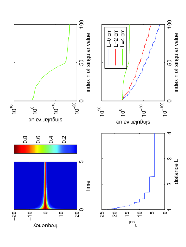
Figure 5: Case: $\gamma=1.66$ (castor oil). The upper left and right pictures visualize the kernel $\mathcal{F}\left\{\mathcal{M}\right\}(\omega,t^{\prime})$ and its singular values for $L:=R_{0}-R=0cm$. The lower right and left pictures visualize $\mathcal{F}\left\{\mathcal{M}\right\}(\omega,t^{\prime})$ for the detector distances $L=0\cdot cm$, $L=2\cdot cm$ and $L=4\cdot cm$ and the respective indices $n_{cut}$ for which the singular values are about $0.1$ per cent of the maximal singular value.

Example 3

An analogous numerical example as in Example 2 for the case $\gamma=1.1$ is presented in Fig. 6. From the lower left picture of Fig. 6, we see that if the distance is about $2\cdot cm$ from the boundary of the object, then $17$ singular values are available for the numerical estimation.

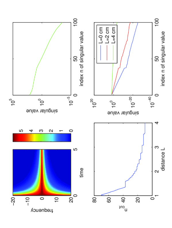
Figure 6: Case: $\gamma=1.1$. The upper left and right pictures visualize the kernel $\mathcal{F}\left\{\mathcal{M}\right\}(\omega,t^{\prime})$ and its singular values. The lower right and left pictures visualize $\mathcal{F}\left\{\mathcal{M}\right\}(\omega,t^{\prime})$ for the detector distances $L=0\cdot cm$, $L=2\cdot cm$ and $L=4\cdot cm$ and the respective indices $n_{cut}$ for which the singular values are about $0.1$ per cent of the maximal singular value.

Example 4

An analogous numerical example as in Example 2 for the case $\gamma=2$ is presented in Fig. 7. From the lower left picture of Fig. 7, we see that if the distance is about $2\cdot cm$ from the boundary of the object, then only $4$ singular values are available for the numerical estimation.

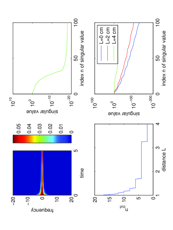
Figure 7: Case: $\gamma=1.1$. The upper left and right pictures visualize the kernel $\mathcal{F}\left\{\mathcal{M}\right\}(\omega,t^{\prime})$ and its singular values. The lower right and left pictures visualize $\mathcal{F}\left\{\mathcal{M}\right\}(\omega,t^{\prime})$ for the detector distances $L=0\cdot cm$, $L=2\cdot cm$ and $L=4\cdot cm$ and the respective indices $n_{cut}$ for which the singular values are about $0.1$ per cent of the maximal singular value.

Example 5

An analogous numerical example as in Example 2 for the frequency power law

$$\alpha_{*}(\omega)=\alpha_{0}^{pl}\cdot(-{\mathrm{i}}\,\,\omega)^{0.66}\qquad\quad(\mbox{$\alpha_{0}^{pl}$ as in Example~{}\ref{exam:distance2}})$$

is presented in Fig. 8. From the lower left picture of this figure, we see that if the distance is about $2\cdot cm$ from the boundary of the object, then $77$ singular values are available for the numerical estimation. If the distance is about $4cm$, then $46$ singular values are available.

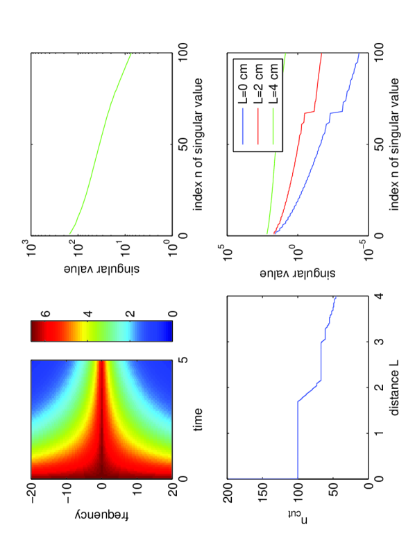
Figure 8: Case: $\gamma=0.66$. The upper left and right pictures visualize the kernel $\mathcal{F}\left\{\mathcal{M}\right\}(\omega,t^{\prime})$ and its singular values. The lower right and left pictures visualize $\mathcal{F}\left\{\mathcal{M}\right\}(\omega,t^{\prime})$ for the detector distances $L=0\cdot cm$, $L=2\cdot cm$ and $L=4\cdot cm$ and the respective indices $n_{cut}$ for which the singular values are about $0.1$ per cent of the maximal singular value.

Comparing all numerical examples shows that the larger $\gamma$ (stronger attenuation), the more rapidly decrease the singular values.

8 Appendix: Nomenclature and Elementary Facts

•

Sets: $B_{R}$ denotes the open ball with center at $\mathbf{0}$ and radius $R$. $S^{n}\subseteq{\mathbb{R}}^{n}$ denotes the $n$-dimensional unit sphere.

•

Real and Complex Numbers: ${\mathbb{C}}$ denotes the space of complex numbers, ${\mathbb{R}}$ the space of reals. For a complex number $c=a+{\mathrm{i}}\,b$ $a=\Re{(c)}$, $b=\Im{(c)}$ denote the real and imaginary parts, respectively.

•

For a complex number $c$ we denote by $\left|c\right|$ the absolute value and by $\phi\in(-\pi,\pi]$ the argument. That is

$$c=\left|c\right|\exp\left(i\phi\right)\;.$$

As a consequence, when $w=r\,\exp\left({\mathrm{i}}\,\phi\right)$ then

$$w^{\gamma}=\exp\left(\gamma\,\left(\text{log}(r)+{\mathrm{i}}\,\phi\right)\right)\;.$$ (101)

Consequently $w^{\gamma}$ has absolute value $r^{\gamma}$ and the argument is $\gamma\phi$ modulo $2\pi$. In this paper all power functions are defined on ${\mathbb{C}}\backslash{\mathbb{R}}_{-}$. We note that

$$w\in{\mathbb{C}}\backslash{\mathbb{R}}_{-}\quad\mbox{and}\quad\Re(\sqrt{w})>0\qquad\Rightarrow\qquad\Im(w)\,\Im(\sqrt{w})\geq 0\,.$$ (102)

•

Differential Operators: $\nabla$ denotes the gradient. $\nabla\cdot$ denotes divergence, and $\nabla^{2}$ denotes the Laplacian.

•

Product: When we write $\cdot$ between two functions, then it means a pointwise product, it can be a scaler product or if the functions are vector valued an inner product. The product between a function and a number is not explicitly stated.

•

Composition: The composition of operators $\mathcal{A}$ and $\mathcal{B}$ is written as $\mathcal{A}\mathcal{B}$.

•

Special functions:

• The signum function is defined by

  $$\mbox{sgn}:=\mbox{sgn}({\vec{x}}):=\frac{{\vec{x}}}{\left|{\vec{x}}\right|}\;.$$

  In ${\mathbb{R}}^{3}$ it satisfies

  $$\nabla\cdot\mbox{sgn}=\frac{2}{\left|{\vec{x}}\right|}\;.$$ (103)

• The Heaviside function

  $$H:=H(t):=\left\{\begin{array}[]{rcl}0&\text{ for }&t<0\\ 1&\text{ for }&t>0\\ \end{array}\right.$$

  satisfies

  $$H:=\frac{1}{2}(1+\mbox{sgn})\;.$$

• The $\delta$-distribution is the derivative of the Heaviside function at $0$ and is denoted by $\delta_{t}:=\delta_{t}(t)$. In our terminology $\delta_{t}$ denotes a one-dimensional distribution. Sometimes, if the context is clear, we will omit the subscript at the $\delta$-distributions.

• The three dimensional $\delta$-distribution $\delta_{\vec{x}}$ is the tensor product of the three one-dimensional distributions $\delta_{x_{i}}$, $i=1,2,3$. Moreover,

  $$\delta_{{\vec{x}},t}:=\delta_{{\vec{x}},t}({\vec{x}},t)=\delta_{\vec{x}}\cdot\delta_{t},$$ (104)

  is a four dimensional distribution in space and time. If we do not add a subscript $\delta$ denotes a one-dimensional $\delta$-distribution.

• $\chi_{\Omega}$ denotes the characteristic set of $\Omega$, i.e., it attains the value $1$ in $\Omega$ and is zero else.

•

Properties related to functions: $\mbox{supp}(g)$ denote the support of the function $g$, that is the closure of the set of points, where $g$ does not vanish.

•

Derivative with respect to radial components: We use the notation

$$r:=r({\vec{x}})=\left|{\vec{x}}\right|,$$

and denote the derivative of a function $f$, which is only dependent on the radial component $\left|{\vec{x}}\right|$, with respect to $r$ (i.e., with respect to $\left|{\vec{x}}\right|$) by $\cdot^{\prime}$.

Let $\beta=\beta(r)$, then it is also identified with the function $\beta=\beta(\left|{\vec{x}}\right|)$ and therefore

$$\nabla\beta=\frac{{\vec{x}}}{\left|{\vec{x}}\right|}\beta^{\prime}\;.$$

•

Convolutions: Three different types of convolutions are considered: $*_{t}$ and $*_{\omega}$ denote convolutions with respect to time and frequency, respectively. Let $f$, $\hat{f}$, $g$ and $\hat{g}$ be functions defined on the real line with complex values. Then

$$f*_{t}g:=\int_{\mathbb{R}}f(t-t^{\prime})g(t^{\prime})dt^{\prime},\quad\quad \hat{f}*_{\omega}\hat{g}:=\int_{\mathbb{R}}\hat{f}(\omega-\omega^{\prime})\hat{g}(\omega^{\prime})d\omega^{\prime}.$$

$*_{{\vec{x}},t}$ denotes space–time convolution and is defined as follows: Let $f,g$ be functions defined on the Euclidean space ${\mathbb{R}}^{3}$ with complex values, then

$$f*_{{\vec{x}},t}g:=\int_{{\mathbb{R}}^{3}}\int_{\mathbb{R}}f({\vec{x}}-{\vec{x}}^{\prime},t-t^{\prime})g({\vec{x}}^{\prime},t^{\prime})d{\vec{x}}^{\prime}dt^{\prime}\;.$$

•

Fourier transform: For more background we refer to L (64); T (48); P (62); Y (95); H (03). All along this paper $\mathcal{F}\left\{\cdot\right\}$ denotes the Fourier transformation with respect to $t$, and the inverse Fourier transform $\mathcal{F}^{-1}\left\{\cdot\right\}$ is with respect to $\omega$. In this paper we use the following definitions of the transforms:

$$\mathcal{F}\left\{f\right\}(\omega) =\frac{1}{\sqrt{2\pi}}\int_{\mathbb{R}}\exp\left({\mathrm{i}}\,\omega t\right)f(t)dt\,,$$

$$\mathcal{F}^{-1}\left\{\hat{f}\right\}(t) =\frac{1}{\sqrt{2\pi}}\int_{\mathbb{R}}\exp\left(-{\mathrm{i}}\,\omega t\right)\hat{f}(\omega)d\omega\;.$$

The Fourier transform and its inverse have the following properties:

1. $$\mathcal{F}\left\{\frac{\partial}{\partial t}f\right\}(\omega)=(-{\mathrm{i}}\,\omega)\mathcal{F}\left\{f\right\}(\omega)\;.$$

2. $$\mathcal{F}\left\{f\cdot g\right\} =\frac{1}{\sqrt{2\pi}}\mathcal{F}\left\{f\right\}*_{\omega}\mathcal{F}\left\{g\right\}\text{ and }$$

   $$\mathcal{F}\left\{f\right\}\cdot\mathcal{F}\left\{g\right\} =\frac{1}{\sqrt{2\pi}}\mathcal{F}\left\{f*_{t}g\right\},$$

   $$\mathcal{F}^{-1}\left\{\hat{f}\cdot\hat{g}\right\} =\frac{1}{\sqrt{2\pi}}\mathcal{F}^{-1}\left\{\hat{f}\right\}*_{t}\mathcal{F}^{-1}\left\{\hat{g}\right\}\text{ and }$$

   $$\mathcal{F}^{-1}\left\{\hat{f}\right\}\cdot\mathcal{F}^{-1}\left\{\hat{g}\right\} =\frac{1}{\sqrt{2\pi}}\mathcal{F}^{-1}\left\{\hat{f}*_{\omega}\hat{g}\right\}\;.$$

3. For $a\in{\mathbb{R}}$

   $$\mathcal{F}\left\{f(t-a)\right\}(\omega)=\exp\left(ia\omega\right)\cdot\mathcal{F}\left\{f(t)\right\}(\omega)$$

4. The $\delta$-distribution at $a\in{\mathbb{R}}$ satisfies

   $$\delta_{t}(t-a)=\frac{1}{\sqrt{2\pi}}\mathcal{F}^{-1}\left\{\exp({\mathrm{i}}\,a\omega)\right\}(t)\;.$$

5. Let $f$ be real and even, odd respectively, then $\mathcal{F}\left\{f\right\}$ is real and even, imaginary and odd, respectively.

6. The Fourier transformation of a tempered distribution is a tempered distribution.

7. Let $\tau_{1},\,\tau_{2}\in{\mathbb{R}}$. If $f_{1}$ and $f_{2}$ are two distributions with support in $[\tau_{1},\infty)$ and $[\tau_{2},\infty)$, respectively, then $f_{1}*f_{2}$ is well-defined and (cf.  H (03))

   $$\mbox{supp}(f_{1}*f_{2})\subseteq\mbox{supp}(f_{1})+\mbox{supp}(f_{2})\subseteq[\tau_{1}+\tau_{2},\infty)\,.$$ (105)

•

The Hilbert transform for $L^{2}-$functions is defined by

$$\mathcal{H}\left\{f\right\}(t)=\frac{1}{\pi}\mathchoice{{\vbox{\hbox{$\textstyle-$}}\kern-4.86108pt}}{{\vbox{\hbox{$\scriptstyle-$}}\kern-3.25pt}}{{\vbox{\hbox{$\scriptscriptstyle-$}}\kern-2.29166pt}}{{\vbox{\hbox{$\scriptscriptstyle-$}}\kern-1.875pt}}\!\int_{\mathbb{R}}\frac{f(s)}{t-s}ds\;,$$

where $\mathchoice{{\vbox{\hbox{$\textstyle-$}}\kern-4.86108pt}}{{\vbox{\hbox{$\scriptstyle-$}}\kern-3.25pt}}{{\vbox{\hbox{$\scriptscriptstyle-$}}\kern-2.29166pt}}{{\vbox{\hbox{$\scriptscriptstyle-$}}\kern-1.875pt}}\!\int_{\mathbb{R}}f(s)ds$ denotes the Cauchy principal value of $\int_{\mathbb{R}}f(s)ds$.

A more general definition of the Hilbert transform can be found in BW (66). The Hilbert transform satisfies

• $\mathcal{H}\left\{\mathcal{F}\left\{f\right\}\right\}(\omega)=-i\mathcal{F}\left\{\mbox{sgn}f\right\}(\omega)$,

• $\mathcal{H}\left\{\mathcal{H}\left\{f\right\}\right\}=-f$.

From the first of these properties the Kramers-Kronig relation can be formally derived as follows. Since $f(t)$ is a causal function if and only if $f=H\cdot f$ and $H=(1+\mbox{sgn})/2$, it follows that $\mathcal{F}\left\{f\right\}=[\mathcal{F}\left\{f\right\}+{\mathrm{i}}\,\mathcal{H}\left\{\mathcal{F}\left\{f\right\}\right\}]/2$, which is equivalent to $\mathcal{F}\left\{f\right\}=i\mathcal{H}\left\{\mathcal{F}\left\{f\right\}\right\}$, i.e.

$$\Re(\mathcal{F}\left\{f\right\})=-\Im(\mathcal{H}\left\{\mathcal{F}\left\{f\right\}\right\})\qquad\text{and}\qquad\Im(\mathcal{F}\left\{f\right\})=\Re(\mathcal{H}\left\{\mathcal{F}\left\{f\right\}\right\}).$$

•

The inverse Laplace transform of $f$ is defined by

$$\mathcal{L}^{-1}\left\{f\right\}(t)=\left\{\begin{array}[]{ccl}0&\text{ for }&t<0,\\ \frac{1}{2\pi i}\int_{\gamma-i\infty}^{\gamma+{\mathrm{i}}\,\infty}\exp\left(st\right)f(s)ds,&\text{ for }&t>0,\end{array}\right.$$

where $\gamma$ is appropriately chosen.

The inverse Laplace transform satisfies (see e.g. H (91))

$$\mathcal{L}^{-1}\left\{h(s-a)\right\}(t)=\exp\left(at\right)\mathcal{L}^{-1}\left\{h(s)\right\}(t)\text{ for all }a,t\in{\mathbb{R}}$$ (106)

and

$$\mathcal{L}^{-1}\left\{s^{-r}\right\}(t)=\frac{H(t)t^{r-1}}{\Gamma(r)}\qquad(r>0)\;.$$ (107)

References

• AK (07) Agranovsky, M. and Kuchment, P.: Uniqueness of reconstruction and an inversion procedure for thermoacoustic and photoacoustic tomography with variable sound speed, Inv. Probl. vol.23, No. 5, 2089–2102, 2007.
• BW (66) Beltrami, E. J. and Wohlers, M. R.: Distributions and the Boundary Values of Analytic Functions. Academic Press, New York and London, 1966.
• BBGHP (07) Burgholzer, P. and Bauer-Marschallinger, J. and Grün, H. and Haltmeier, M. and Paltauf, G.: Temporal back-projection algorithms for photoacoustic tomography with integrating line detectors. Inverse Probl., 23(6):65-80, 2007.
• BGHNP (07) Burgholzer, P. and Grün, H. and Haltmeier, M. and Nuster, R. and Paltauf, G.: Compensation of acoustic attenuation for high-resolution photoacoustic imaging with line detectors. In A.A. Oraevsky and L.V. Wang, editors, Photons Plus Ultrasound: Imaging and Sensing 2007: The Eighth Conference on Biomedical Thermoacoustics, Optoacoustics, and Acousto-optics, volume 6437 of Proceedings of SPIE, page 643724. SPIE, 2007.
• BRBP (010) Burgholzer, P., Roitner, H., Bauer-Marschallinger, J., Paltauf, G.: Image Reconstruction in Photoacoustic Tomography Using Integrating Detectors Accounting for Frequency-Dependent Attenuation. Volume 7564, page 75640O. Proc. SPIE, 2010.
• CH (04) Chen, W and Holm, S.: Fractional Laplacian time-space models for linear and nonlinear lossy media exhibiting arbitrary frequency power-law dependency. J. Acoust. Soc. Am. 115 (4), April 2004.
• CPW (90) Cheong, W. F. and Prahl, S. A. and Welch, A. J.: A review of the optical properties of biological tissues. IEEE J. Quantum Electron., 26(12):2166–2185, 1990.
• (8) Dautray, R. and Lions, J.-L.: Mathematical Analysis and Numerical Methods for Science and Technology. Volume 1. Springer-Verlag, New York, 2000.
• (9) Dautray, R. and Lions, J.-L.: Mathematical Analysis and Numerical Methods for Science and Technology. Volume 2. Springer-Verlag, New York, 2000.
• (10) Dautray, R. and Lions, J.-L.: Mathematical Analysis and Numerical Methods for Science and Technology. Volume 5. Springer-Verlag, New York, 2000.
• FPR (04) Finch, D. and Patch, S. and Rakesh: Determining a function from its mean values over a family of spheres. Siam J. Math. Anal. Vol. 35, No. 5, pp. 1213-1240.
• GW (99) Gasquet, C and Witomski, P: Fourier Analysis and Applications. Springer-Verlag, New York, 1999.
• GK (93) Gusev, V. E. and Karabutov, A. A.: Laser Optoacoustics. American Institute of Physics, New York, 1993.
• HSBP (04) Haltmeier, M. and Scherzer, O. and Burgholzer, P. and Paltauf, P.: Thermoacoustic imaging with large planar receivers. Inverse Probl., 20(5):1663-1673, 2004.
• HS (03) Hanyga, A. and Seredynska, M.: Power-law attenuation in acoustic and isotropic anelastic media. Geophys. J. Int, 155:830-838, 2003.
• H (91) H. Heuser. Gewöhnliche Differentialgleichungen. Teubner, Stuttgart, second edition, 1991.
• H (03) Hörmander, L.: The Analysis of Linear Partial Differential Operators I. Springer Verlag, New York, 2nd edition, 2003.
• HKN (08) Hristova, Y. and Kuchment, P. and Nguyen, L.: Reconstruction and time reversal in thermoacoustic tomography in acoustically homogeneous and inhomogeneous media. Inverse Problems, 24(5):055006 (25pp), 2008.
• J (82) John, F.: Partial Differential Equations. Springer Verlag, New York, 1982.
• KST (06) Kilbas, A.A. and Srivastava, H.M. and Trujillo, J.J.: Theory and applications of fractional differential equations, volume 204 of North-Holland Mathematics Studies. Elsevier Science B.V., Amsterdam, 2006.
• KFCS (00) Kinsler, L. E., Frey, A. R., Coppens, A. B., Sanders, J. V.: Fundamentals of Acoustics. Wiley, New York, 2000.
• KSB (10) Kowar, R . and Scherzer, O. and Bonnefond, X.: Causality analysis of frequency-dependent wave attenuation. to apper in: Math. Meth. Appl. Sci. 2010, DOI: 10.1002/mma.1344
• KKMR (00) Kruger, R. A. and Kiser, W. L. and Miller, K. D. and Reynolds, H. E.: Thermoacoustic CT: imaging principles. Proc. SPIE 2000, vol. 3916, 150–159.
• KWSW (04) Ku, G. and Wang, X. and Stoica, G. and Wang, L. V.: Multiple-bandwidth photoacoustic tomography. Phys. Med. Biol., 49:1329–1338, 2004.
• KK (07) Kunyansky, L. A.: Explicit inversion formulae for the spherical mean Radon transform. Inverse Probl., 23,373-383, 2007.
• KK (08) Kuchment, P., Kunyansky, L. A.: Mathematics of thermoacoustic and photoacoustic tomography. European J. Appl. Math., 19:191–224, 2008.
• LL (91) Landau, L. D. and E.M. Lifschitz, E. M.: Lehrbuch der theoretischen Physik, Band VII: Elastizitätstheorie. Akademie Verlag, Berlin, 1991.
• L (64) Lighthill, M.J.: Introduction to Fourier Analysis and Generalized Functions. Student’s Edition. Cambridge University Press, London, 1964.
• NSW (90) Nachman, A. I. and Smith, J. F., III and Waag, R. C.: An equation for acoustic propagation in inhomogeneous media with relaxation losses. J. Acoust. Soc. Am. 88 (3), Sept. 1990.
• OW (07) Oraevsky, A. and Wang, L.V., editors: Photons Plus Ultrasound: Imaging and Sensing 2007: The Eighth Conference on Biomedical Thermoacoustics, Optoacoustics, and Acousto-optics, volume 6437 of Proceedings of SPIE, 2007.
• PS (07) Patch, S. K. and Scherzer, O.: Special section on photo- and thermoacoustic imaging. Inverse Probl., 23:S1–S122, 2007.
• PG (06) Patch, S. K. and Greenleaf, A.: Equations governing waves with attenuation according to power law. Technical report, Department of Physics, University of Wisconsin-Milwaukee, 2006.
• P (62) Papoulis, A.: The Fourier Integral and its Applications. McGraw-Hill, New York, 1962.
• P (99) Podlubny, I.: Fractional differential equations, volume 198 of Mathematics in Science and Engineering. Academic Press Inc., San Diego, CA, 1999.
• (35) Razansky, D. and Distel, M. and Vinegoni, C. and Ma, R. and Perrimon, N. and Köster, R. W. and Ntziachristos, V.: Multispectral opto-acoustic tomography of deep-seated fluorescent proteins in vivo, Nature Photonics 3: 412-417, 2009.
• RZA (06) La Riviére, P. J. and Zhang, J. and Anastasio, M. A.: Image reconstruction in optoacoustic tomography for dispersive acoustic media. Opt. Letters, 31(6):781–783, 2006.
• SGLGH (09) Scherzer, O. and Grossauer, H. and Lenzen, F. and Grasmair, M. and Haltmeier, M.: Variational Methods in Inmaging. Springer-Verlag, New York, 2009.
• SC (04) Sushilov, N. V. and Cobbold, R. S. C.: Frequency-domain wave equation and its time-domain solution in attenuating media. Journal of the Acoustical Society of America, 115:1431–1436, 2005.
• S (94) Szabo, T. L.: Time domain wave equations for lossy media obeying a frequency power law. J. Acoust. Soc. Amer., 96:491–500, 1994.
• S (95) Szabo, T. L.: Causal theories and data for acoustic attenuation obeying a frequency power law. J. Acoust. Soc. Amer., 97:14–24, 1995.
• T (86) Tam, A. C.: Applications of photoacoustic sensing techniques. Rev. Modern Phys., 58(2):381–431, 1986.
• T (48) Titchmarch, E. C.: Theory of Fourier Integrals. Clarendon Press, Oxford, 1948.
• WHBM (00) Waters, K. R. and Hughes, M. S. and Brandenburger, G. H. and Miller, J. G.: On a time-domain representation of the Kramers-Krönig dispersion relation. J. Acoust. Soc. Amer., 108(5):2114–2119, 2000.
• WMM (05) Waters, K.R. and Mobely, J. and Miller, J. G.: Causality-Imposed (Kramers-Krönig) Relationships Between Attenuation and Dispersion. IEEE Trans. Ultrason., Ferroelect., Freq. Contr., vol. 52, no. 5, May 2005.
• W (00) Webb, S., editor: The Physics of Medical Imaging. Institute of Physics Publishing, Bristol, Philadelphia, 2000. reprint of the 1988 edition.
• W (08) Wang, L. V.: Prospects of photoacoustic tomography. Med. Phys., 35(12):5758–5767, 2008.
• WPKXS (03) Wang, X. D. and Pang, Y. J. and Ku, G. and Xie, X. Y. and Stoica, G. and Wang, L. V.: Noninvasive Laser-Induced Photoacoustic Tomography for Structural and Functional in Vivo Imaging of the Brain 2003, vol. 21, No. 7, 803–806
• XFW (02) Xu, Y. and Feng, D. and Wang, L. V.: Exact Frequency-Domain Reconstruction for Thermoacoustic Tomography - I: Planar Geometry. IEEE Trans. Med. Imag., Vol. 21, N0. 7, July 2002.
• XXW (02) Xu, Y. and Xu, M. and Wang, L. V.: Exact Frequency-Domain Reconstruction for Thermoacoustic Tomography - II: Cylindrical Geometry. IEEE Trans. Med. Imag., Vol. 21, N0. 7, July 2002.
• XXW (03) Xu, M. and Xu, Y. and Wang, L. V.: Time-Domain Reconstruction Algorithms and Numerical Simulation for Thermoacoustic Tomography in Various Geometries. IEEE Trans. Biomed. Eng., Vol. 50, N0. 9, Sept. 2003.
• XWAK (03) Xu, Y. and Wang, L. V. and Ambartsoumian, G. and Kuchment, P.: Reconstructions in limited-view thermoacoustic tomography. Med. Phys., 31 (4), April 2004.
• XW (05) Xu, M. and Wang, L. V.: Universal back-projection algorithm for photoacoustic computed tomography. Phys. Rev. E 71, 2005. Article ID 016706.
• XW (06) Xu, M. and Wang, L. V.: Photoacoustic imaging in biomedicine. Rev. Sci. Instruments, 77(4):1–22, 2006. Article ID 041101.
• Y (95) Yosida, K.: Functional analysis. Springer-Verlag, Berlin, Heidelberg, New York 1995, 5th edition
• ZLB (07) Zhang, E.Z. and Laufer, J. and Beard, P.: Three-dimensional photoacoustic imaging of vascular anatomy in small animals using an optical detection system. In OW (07), 2007.
• ZMSW (06) Zhang, H. and Maslov, K. and Stoika, G. and Wang. V.L.: Functional photoacoustic microscopy for high-resolution and noninvasive in vivo imaging. Nat. Biotechnol., 24:848 – 851, 2006.
Index
• absorption energy §1
• attenuation §2
• attenuation coefficient Definition 1
• attenuation coefficient, standard Definition 1
• attenuation coefficient, $\beta^{*}$ §2
• attenuation law Definition 1
• attenuation law, KSB (10), $\alpha_{ksb}^{*}$ 7th item
• attenuation law, Greenleaf & Patch, $\alpha_{gp}^{*}$ 5th item
• attenuation law, Nachman & Smith & Waag, $\alpha_{nsw}^{*}$ 4th item
• attenuation law, power law, $\alpha_{pl}^{*}$ 1st item, 2nd item
• attenuation law, Szabo, $\alpha_{sz}^{*}$ 2nd item
• attenuation law, thermo-viscous, $\alpha_{tv}^{*}$ 3rd item
• ${\mathbb{C}}_{0}$ item 1
• convolution kernel, $K$ §2
• ${\mathbb{C}}_{\varepsilon}$ §4
• $\mathcal{D}$ 1st item
• $D_{*}$ §5
• finite speed of propagation 5th item
• Function, causal Definition 2
• Function, rapidly decreasing 2nd item
• Green function Definition 3
• Green function, standard wave equation 7
• $K_{*}$ §5
• $\mathcal{M}$ §6
• Operator, causal 3rd item
• Operator, rotation invariant 2nd item
• Operator, shift invariant 1st item
• Operator, strongly causal 6th item
• $p_{\text{att}}$ §5
• Riemann-Liouville fractional derivative, $D_{t}^{\gamma}$ 1st item
• $\mathcal{S}$ 2nd item
• source term, photoacoustic model §1
• tempered distributions, $\mathcal{S}^{\prime}$ 4th item
• travel time of a wave front 1st item
• wave equation §1
• wave equation, photoacoustic model §1
• wave front 3rd item
• wave front speed 4th item