Tripartite thermal correlations in an inhomogeneous spin-star system

Abstract

We exploit the tripartite negativity to study the thermal correlations in a tripartite system, that is the three outer spins interacting with the central one in a spin-star system. We analyze the dependence of such correlations on the homogeneity of the interactions, starting from the case where central-outer spin interactions are identical and then focusing on the case where the three coupling constants are different. We single out some important differences between the negativity and the concurrence.

I Introduction

The notion of thermal entanglement relies on the amount of entanglement possessed by a physical system when it had undergone a thermalization process that has brought it in a thermal state ref:Arnesen2001 . In fact, in the presence of interaction between different parts of a compound system, even after a complete thermalization, the system can exhibit appreciable quantum correlations since the Hamiltonian eigenstates are, in general, entangled states. The establishment of a relation between temperature and entanglement has quickly brought to the idea of using the entanglement as an order parameter in quantum phase transitions ref:Osterloh2002 ; ref:Osborne2002 . Moreover, it has given a stronger stimulus of searching quantum correlations in the macroscopic world ref:Vedral2004 ; ref:Vedral2005 ; ref:Vedral2008 .

Thermal entanglement has been studied in connection with many possible applications and in different physical systems: detailed analysis in spin chains described by Heisenberg models has been given ref:Gong2009 as well as in atom-cavity systems ref:Wang2009 and in simple molecular models ref:Pal2010 . The quantumness of correlations has been singled out in thermalized spin chains ref:Werlang2010 also in connection with non local effects ref:Souza2009 , and application of thermal entanglement in optimal quantum teleportation protocols has been proposed ref:Zhou2009 .

Spin systems have been studied in depth not only in the neighbor-interaction configuration, leading to the Heisenberg model, but also in star networks. This kind of systems can be realized in many physical contexts, from Josephson Junctions ref:Makhlin1999 to trapped ions ref:Cirac2000 to solid state physics ref:Keane1998 . In 2004, Hutton and Bose have analyzed a physical system made of a central spin interacting with a set of $N$ outer spins at zero temperature, bringing to light interesting properties which are immediately traceable back to the features of the ground state of this spin-star network ref:Hutton2004 . They have shown that the evenness or oddness of the number of outer spins determines the law the entanglement amount scales with. The same spin configuration, in a simplified version involving three outer spins only, has been recently considered by Wan-Li et al ref:Wan-Li2009 in the special case where all the interactions between the central spin and the outer ones are identical. Exploiting the high degree of symmetry of the system, they concentrate on appropriate concurrences ref:Wootters to extract information about the presence of quantum correlations. However, the disclosure of quantum correlations in tripartite systems could require tools and concepts more adequate than the simple concurrences. Sabin and Garcia-Alcaine have contributed to solve this still very open problemref:Fazio2008 introducing the notion of tripartite negativityref:Sabin2008 , which is an effective tool to reveal the existence of quantum correlations traceable back to the impossibility of separating any of the three subsystems from the other two.

In this paper we consider a spin-star system where three outer spins are coupled to the central one with different strengths, and analyze thermal entanglement in different situations. In the next section we present the model under scrutiny, which is characterized by anisotropic spin-spin interactions due to the absence of longitudinal $z$-$z$ couplings. In the third section we consider the system in the homogeneous case, showing the presence of sharp changes in the amount of entanglement at zero temperature due to abrupt variations of the ground state. In the fourth section we analyze the inhomogeneous model, focusing on two types of inhomogeneity. Finally, in the last section some comments and conclusive remarks are given.

II Physical scenario

System and Hamiltonian -

In this section we present the spin star-system we have analyzed, which is pictured in Fig. 1. Numbers $1,2,3$ indicate the three outer spin $1/2$, while the central one is indicated with latin capital letter $C$. With $c_{1},c_{2}$ and $c_{3}$ we indicate the coupling constants of the central spin with the outer spin $1$, $2$ and $3$, respectively. Moreover, the whole system is immersed in a constant uniform magnetic field of modulus $B_{0}$ and directed along the $z$-axis. The Hamiltonian model is then given by (with $\hbar=1$):

$$\mathbf{H}=\mathbf{H_{1}}+\mathbf{H_{2}}\;,$$ (1)

$$\mathbf{H_{1}}=-\frac{\gamma_{s}}{2}B_{0}\sum_{i}\sigma_{z}^{i}=\frac{\omega_{0}}{2}\sum_{i}\sigma_{z}^{i}\;,$$ (2)

$$\mathbf{H_{2}}=\sum_{i=1,2,3}c_{i}\left(\sigma_{+}^{C}\sigma_{-}^{i}+\sigma_{-}^{C}\sigma_{+}^{i}\right)\;,$$ (3)

where $\sigma_{z}^{i}=\left|+\right\rangle_{i}\left\langle+\right|-\left|-\right\rangle_{i}\left\langle-\right|$, $\sigma_{+}^{i}=\left|+\right\rangle_{i}\left\langle-\right|$, $\sigma_{-}^{i}=\left|-\right\rangle_{i}\left\langle+\right|$, $\omega_{0}$ is the unperturbed Bohr frequency, and $c_{i}$’s are coupling constants.

The term $\mathbf{H_{1}}$, describes the interaction of the system with the magnetic field, while the second one, $\mathbf{H_{2}}$, arises from the dipole-like interactions between the central spin and the outer ones. The absence of $z$-$z$ interaction reflects a certain degree of anisotropy.

Figure 1: The physical system. Spins labeled 1,2 and 3 are coupled to the central (C) one. The magnetic field $B_{0}$ is ortogonal to the plan where the four spins lie.

Assuming that the system is in a thermal state, its density operator takes the form:

$$\rho=\frac{e^{-\frac{\mathbf{H}}{k_{B}T}}}{\textrm{Tr}\left({e^{-\frac{\mathbf{H}}{k_{B}T}}}\right)}\;=\frac{e^{-\frac{\mathbf{H}}{k_{B}T}}}{Z}\;,$$ (4)

so that $\rho$ and $\mathbf{H}$ share the same eigenstates. The Hamiltonian model given in Eq. (1) takes into account possible inhomogeneities, nevertheless it is surely of interest studying it in the homogeneous case ($c_{1}=c_{2}=c_{3}=c$) which turns out to be simpler from a mathematical point of view, paving the way to the study of the more complicated inhomogeneous model. Wan-Li et al. ref:Wan-Li2009 have analyzed the homogeneous model taking advantage of the concurrence to quantify entanglement. In addition, they have assumed a more general anisotropic interaction. Since in real situations the construction of a system with perfectly homogeneous interactions could be quite difficult, in this paper we investigate the features of thermal quantum correlations in the presence of inhomogeneity.

Tripartite negativity -

Remarking that the analysis is performed on the outer subsystem, which is made of three parts, we have the need to study quantum correlations in tripartite systems. There are various proposals of tripartite entanglement quantifiers ref:TripQuantify-1 ; ref:TripQuantify-2 ; ref:TripQuantify-3 ; ref:TripQuantify-4 and witnesses ref:TripWitnesses-1 ; ref:TripWitnesses-2 ; ref:TripWitnesses-3 , the latter ones based on the key assertions in ref:TripWitnesses . Nevertheless, up to now and to the best of our knowledge, there is not a definitive answer to the request of quantifying tripartite entanglement ref:Fazio2008 . For instance, it has been shown recently that three-tangle ref:ThreeTangle could be an improper tool for such a purpose ref:DoesThreeTangle . The situation is much more complicated when we have to consider mixed states. Indeed, all the recipes mentioned in ref:TripQuantify-1 ; ref:TripQuantify-2 ; ref:TripQuantify-3 ; ref:TripQuantify-4 ; ref:ThreeTangle refer to pure states and fail when applied to non-pure states. Since we are studying thermal correlations, therefore dealing with highly mixed states, we need a tool to investigate quantum correlations in mixed states of tripartite systems. Again, to the best of our knowledge, the tripartite negativity introduced by Sabin and Garcia-Alcaine ref:Sabin2008 is a good quantity that allows to study quantum correlations in tripartite systems, even in the case of mixed states. Other quantities are very much related to the specific structure of the analyzed system, since observables that assume values in a certain range when the state is entangled are considered. Sabin and Garcia-Alcaine apply bipartite negativity to all the three possible bipartitions that can be singled out isolating one subsystem and considering the other two as a whole; then they consider the geometric mean of these three quantities. According to the definition of negativity ref:Zyczkowski ; ref:Vidal , the partial negativity related to the bipartition $I-(JK)$ (in which the two subsystems $J$ and $K$ are considered as a whole) is given by

$$\mathcal{N}_{I-JK}=\sum_{i}|\sigma_{i}(\tau^{TI})|-1\quad,$$ (5)

where $\sigma_{i}(\tau^{TI})$ is the $i$-th eigenvalue of $\tau^{TI}$, which is the partial transpose related to subsystem $I$, of the total ($IJK$) density matrix. The parameter used to study correlations in tripartite systems is then

$$\mathcal{N}_{123}=\sqrt[3]{\mathcal{N}_{1-23}\,\mathcal{N}_{2-13}\,\mathcal{N}_{3-12}}\;,$$ (6)

which is the above mentioned tripartite negativity. In ref:Sabin2008 the following properties have been proven:

• $\tau$ separable or simply bi-separable $\;\Rightarrow\;\mathcal{N}_{123}=0$;

• Invariance of $\mathcal{N}_{123}$ under LU operators;

• Monotonicity of $\mathcal{N}_{123}$ under LOCC operators;

Though $\mathcal{N}_{123}$ is not a sufficient condition to single out tripartite entanglement, it is an effective tool to study quantum correlations in tripartite systems. In fact, finding $\mathcal{N}_{123}\neq 0$ implies that none of the three subsystems is separable, hence revealing correlations involving all the three subsystems. It is also important to note that negativity $\mathcal{N}_{I-JK}$ does involve all the three spins, and establishes the existence of a correlation between $I$ and the entire couple made of $J$ and $K$, which is a very different operation from tracing over one spin, say $K$, and evaluating the degree of correlation between the other two, say $I$ and $J$.

III Homogeneous model

Let us consider our model in the special case $c_{1}=c_{2}=c_{3}=c$ that we have already addressed as the homogeneous case. The complete diagonalization of this Hamiltonian model is given in Appendix A. In order to compute tripartite negativity we need first to find explicit form of the outer-spin density operator $\rho_{123}$, tracing over the degrees of freedom of the central spin.

It is quite clear that because of homogeneity, $\mathcal{N}_{1-23}=\mathcal{N}_{2-13}=\mathcal{N}_{3-12}$, so the geometric mean reduces to one of these three quantities. In Fig. 2 we plot $\mathcal{N}_{123}$ as a function of temperature ($T$) and coupling constant ($c$). One can see some interesting features of $\mathcal{N}_{123}$, for example its diminishing as $T$ increases, and the presence of abrupt transitions at low temperature due to fast variations of the ground state. In Fig. 3, where $\mathcal{N}_{123}(k_{B}T,c=6\omega_{0})$ is plotted, it is better shown this behavior which is due to the fact that the more temperature increases the more $\rho_{C123}$ approaches a maximally mixed states ($\frac{1}{16}\mathbb{I}$), making also $\rho_{123}$ maximally mixed. A more interesting trend of $\mathcal{N}_{123}$ is observed at low temperature where abrupt variations are present, as shown in Fig. 4. At $k_{B}T=0.01\omega_{0}$ fast entanglement variations are well visible at $c\approx 0.6\omega_{0}$ and $c\approx 3.7\omega_{0}$. The reason for this occurrences is that in each of these points the system undergoes a level crossing involving its two lowest levels (ground and first excited states). Let us call $A_{1},A_{2},A_{3}\>$ the three plateaux of Fig. 4, corresponding to $(c<0.6\omega_{0})\>(0.6\omega_{0}<c<3.72\omega_{0})$ and $(c>3.72\omega_{0})$, respectively. The entanglement in these areas is the same of the entanglement possessed by the ground state. In $A_{1}$ entanglement is evidently zero and, in fact, the ground state of the whole system is $\left|g^{(A_{1})}\right\rangle=\left|0000\right\rangle$, corresponding to $\rho_{123}^{(A_{1})}=\left|000\right\rangle\left\langle 000\right|$ (with the notation $\left|\sigma_{C}\,\sigma_{1}\,\sigma_{2}\,\sigma_{3}\right\rangle$). In regions $A_{2}$ and $A_{3}$ ground states of four spin system are $\left|g^{(A_{2})}\right\rangle=$ $\left(\left|0100\right\rangle+\left|0010\right\rangle+\left|0001\right\rangle-\sqrt{3}\left|1000\right\rangle\right)/\sqrt{6}$ and $\left|g^{(A_{3})}\right\rangle=$ $\left(\left(\left|0011\right\rangle+\left|0101\right\rangle+\left|0110\right\rangle\right)\right.$ $-\left.\left(\left|1100\right\rangle+\left|1010\right\rangle+\left|1001\right\rangle\right)\right)/\sqrt{6}$, and the respective density matrix are $\rho_{123}^{(A_{2})}=$ $\left(\left|W\right\rangle\left\langle W\right|+\left|000\right\rangle\left\langle 000\right|\right)/2$ and $\rho_{123}^{(A_{3})}=$ $\left(\left|W\right\rangle\left\langle W\right|+|\tilde{W}\rangle\langle\tilde{W}|\right)/2$, where $|W\rangle=\left(\left|100\right\rangle+\left|010\right\rangle+\left|001\right\rangle\right)/\sqrt{3}$ and $|\tilde{W}\rangle=\left(\left|011\right\rangle+\left|101\right\rangle+\left|110\right\rangle\right)/\sqrt{3}$.

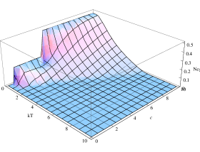
Figure 2: Tripartite negativity $\mathcal{N}_{123}$ for the homogeneous model as a functions of coupling constant ($c$) and temperature ($k_{B}T$), both in units of $\omega_{0}$. Both the diminishing for increasing temperature and the low-temperature transitions with respect to $c$ are well visible.

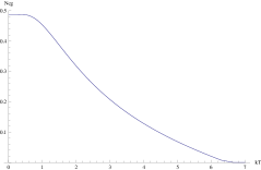
Figure 3: Tripartite negativity $\mathcal{N}_{123}$ of the homogeneous model versus $k_{B}T$, at $c=10\omega_{0}$. Temperature is in units of $\omega_{0}$. In the area where $k_{B}T<\omega_{0}/2$ we observe that the negativity is almost constant.

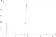
Figure 4: Tripartite negativity $\mathcal{N}_{123}$ of the homogeneous model versus coupling constants (in units of $\omega_{0}$), at $k_{B}T=0.01\omega_{0}$. Abrupt variations at $c\approx 0.6\omega_{0}$ and $c\approx 3.7\omega_{0}$ are well visible. Three plateaux, $A_{1}\>(c<0.6\omega_{0}),A_{2}\>(0.6\omega_{0}<c<3.72\omega_{0}),A_{3}\>(c>3.72\omega_{0})$ are quite evident.

IV Inhomogeneous model

Once we have analyzed the homogeneous model, we turn to the study of the lack of homogeneity in the three interactions. For the sake of simplicity we shall concentrate on two kinds of inhomogeneity that we call type A ($c_{1}=c$, $c_{2}=c\,x$, $c_{3}=c$) and type B ($c_{1}=c$, $c_{2}=c\,x$, $c_{3}=c\,x^{2}$), in both of which the inhomogeneity is characterized by a suitable dimensionless real parameter $x$. In both cases we study the thermal quantum correlations of the tripartite outer subsystem as a function of temperature ($T$), coupling parameter ($c$), and parameter of inhomogeneity ($x$). It is worth noting that in the homogeneous model the structure of eigenstates of $\mathbf{H}$ is independent on the coupling constant ($c$), so that the features of the correlations are essentially determined by the structure of the eigenvalues only. Instead, in the inhomogeneous case the eigenvalues are $c-$ and $x-$dependent and the eigenstates depend on $x$, therefore the thermal correlations are affected both by the crossing of levels and by the modification of the structure of the eigenstates. We will see that while the change of the eigenstates produces smooth changes of $\mathcal{N}_{123}$, on the other hand a level crossing, especially at low temperature, can produce a very sharp variation of the negativity.

IV.1 Model with inhomogeneity of type A

In spite of the lack of some symmetry, the inhomogeneous model of type A is still easily solvable and its diagonalization is given in Appendix A.

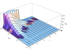
Figure 5: Negativity $\mathcal{N}_{123}$ versus temperature ($k_{B}T$, in units of $\omega_{0}$) and inhomogeneity parameter ($x$), at $c=6\omega_{0}$, for the inhomogeneous model of type A. The trend with respect to temperature is decreasing. The dependence of $\mathcal{N}_{123}$ on the inhomogeneity parameter, at low temperature, exhibits different trends: initially, smooth changes, then, fast falling around $x\approx 5.5$ and zero value from there on.

Since one can see that in the Area $A_{3}$ of Fig. 4 negativity assumes its greatest value, we start the analysis of the inhomogeneous model of type A showing in Fig. 5 the complete dependence of $\mathcal{N}_{123}$ on temperature and inhomogeneity parameter for $c=6\omega_{0}$ (this specific value of $c$ belongs indeed to the area $A_{3}$ of the homogeneous model). It is quite obvious that the physical reason of the decreasing of $\mathcal{N}_{123}$ with respect to $T$ is the same as for the homogeneous case, i.e. the high degree of mixedness. At low temperature, in the $0<x<1$ area, the smaller is $x$, the closer to zero is the negativity. In fact, when $x$ is quite smaller than $1$, $c_{2}=c\>x$ is much smaller than $c_{1}=c_{3}=c$, and hence, roughly speaking, spin $2$ can be considered almost decoupled, and then separable. Moreover, at $x_{0}\approx 0.43$ this negligibility of the coupling between spin $C$ and spin $2$ is concomitant to a level crossing between the two lowest energy levels, $E_{2}^{-}(c=6\omega_{0},x)=-3\omega_{0}\left(x+\sqrt{8+x^{2}}\right)$ and $E_{4}^{-}(c=6\omega_{0},x)=-(6\sqrt{2+x^{2}}+1)\,\omega_{0}$, that causes a sharp change at $x=x_{0}$, where $E_{2}^{-}=E_{4}^{-}$.

Still, at low temperature, for $x$ quite greater than $1$, $\mathcal{N}_{123}$ decreases as $x$ becomes increasingly grater than $1$, because the coupling with spin $2$ becomes stronger than the other two, making spin $1$ and $3$ almost separable from the spin $2$. Around $x\approx 5.5$ a level crossing occurs. Because of the diminishing of $\mathcal{N}_{123}$ for $x\gg 1$ and $x\ll 1$, there must be a maximum in the intermediate region. Unexpectfully, this maximum is reached at $x=x_{M}\approx 2.46$, instead of $x=1$. We think this is an important result because, even though there is no big difference in the values of negativity in a wide contour of the maximum (let’s say from $x=0.5$ to $x=5.5$). In fact, it is conceptually important that the maximum of correlations is not reached in the homogeneous case, where the high symmetry of the system could lead to the idea of stronger correlations between its parts.

Evaluating the eigenvalues of Hamiltonian one can find that the ground state in the nearby of this maximum is $\left|\Psi_{2}^{-}\right\rangle$, which becomes $\left|\Psi_{M}^{(A)}\right\rangle\approx 0.2073\left(\left|0011\right\rangle+\left|1100\right\rangle\right)+0.2073\left(\left|1001\right\rangle+\left|0110\right\rangle\right)-0.6435\left(\left|1010\right\rangle+\left|0101\right\rangle\right)$ for $x=x_{M}$. In this region, the values of $\mathcal{N}_{123}$ and in particular the appearance of a maximum are essentially determined by the dependence of the structure of the state $\left|\Psi_{2}^{-}\right\rangle$ on the inhomogeneity parameter. The relevant density operator is a mixture of two Werner-like states, and can be written in the following way:

$$\rho^{2-}(x)=\frac{1}{2}\left|w_{1}(x)\right\rangle\left\langle w_{1}(x)\right|+\frac{1}{2}\left|w_{2}(x)\right\rangle\left\langle w_{2}(x)\right|\,,$$ (7)

with

$$\left|w_{1}(x)\right\rangle = \aleph\left(\left|011\right\rangle+\left|110\right\rangle+\frac{\sqrt{8+x^{2}}-x}{2}\left|101\right\rangle\right)\,,$$ (8)

$$\left|w_{2}(x)\right\rangle = \aleph\left(\left|100\right\rangle+\left|001\right\rangle+\frac{\sqrt{8+x^{2}}-x}{2}\left|010\right\rangle\right)\,,$$ (9)

where

$$\aleph=\left(2+\left((\sqrt{8+x^{2}}-x)/2\right)^{2}\right)^{-1/2}\,.$$ (10)

The relevant negativity can be evaluated and it turns out to be:

$${\cal N}(\rho^{2-}(x))=\frac{1}{2^{5/3}}\left\{-\frac{1}{(8+x^{2})^{3/2}}\right.$$ (11)

$$\times \left.\left[x+\sqrt{8+x^{2}}-\sqrt{2(20+x(x+\sqrt{8+x^{2}}))}\right]\right.$$

$$\times \left.\left[x-3\sqrt{8+x^{2}}+8\sqrt{8+x^{2}}\right.\right.$$

$$\times \left.\left.\left(|\lambda_{1}(x)|+|\lambda_{2}(x)|+|\lambda_{3}(x)|\right)\right]^{2}\right\}^{1/3}$$

with $\lambda_{i}(x)$’s the roots of the algebraic equation in $\lambda$:

$$\left(-10x+x^{3}+(2+x^{2})\sqrt{8+x^{2}}\right)$$

$$+\left(-32x-4x^{3}-48\sqrt{8+x^{2}}-4x^{2}\sqrt{8+x^{2}}\right)\lambda$$

$$+\left(128x+16x^{3}-384\sqrt{8+x^{2}}-48x^{2}\sqrt{8+x^{2}}\right)\lambda^{2}$$

$$+\left(1024\sqrt{8+x^{2}}+128x^{2}\sqrt{8+x^{2}}\right)\,\lambda^{3}\,=\,0\,,$$ (12)

where the coefficients, and hence the solutions, depend on $x$. The behavior of ${\cal N}(\rho^{2-}(x))$ is shown in fig. 6, where the negativity of the thermal state for $c=6\omega_{0}$ and $T\approx 0$ versus $x$ has also been plotted. It is well visible that the behavior of ${\cal N}(\rho^{2-}(x))$ perfectly reproduces the edge of the top visible in fig. 5 in the low temperature region and for $x$ belonging to the region where $\left|\Psi_{2}^{-}\right\rangle$ is the ground state of the system.

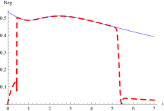
Figure 6: Comparison of the Negativity ${\cal N}(\rho^{2-}(x))$ (solid blue line) with the Negativity of the thermal state (dashed red line) evaluated for $c=6\omega_{0}$ and $k_{B}T=0.01\omega_{0}$, both vs $x$. In the region $0.5<x<5.5$ (where $\left|\Psi_{2}^{-}\right\rangle$ is the ground state) the two curves coincide.

It could be interesting to compare the behavior of the tripartite negativity with the values of the three concurrences related to the three couples of spins that can be extracted tracing over one of them: ${\cal C}_{23}={\cal C}(\textrm{Tr}_{1}\rho^{2-})$, ${\cal C}_{12}={\cal C}(\textrm{Tr}_{3}\rho^{2-})$, ${\cal C}_{13}={\cal C}(\textrm{Tr}_{2}\rho^{2-})$. Figure 7 shows that around $x=0.5$ and $x=5.5$ there are abrupt changes in the values of the concurrences (in the same points where the tripartite negativity exhibits the same behavior), due to rapid changes of the ground state. It is worth noting that in the region $3.5-5.5$ the concurrences $C_{12}$ and $C_{23}$ are vanishing while the tripartite negativity (and hence all the three relevant bipartite Negativity functions) is not. This apparent contradiction reflects the very different meanings of these quantities. Indeed, for example, while the concurrence $C_{12}$ measures the entanglement between spins $1$ and $2$, without considering the spin $3$ that has been preliminarily traced over, the negativity ${\cal N}_{1-23}$ takes into account the correlations between spin $1$ and the whole couple made of the two spins $2$ and $3$. Therefore, in that region, we can talk about correlations between spin $1$ and the couple $(2,3)$ without correlations between $1$ and any of the other two spins, after the third has been traced over. We think this is an important result, since it underlines the difference between ${\cal N}$ and ${\cal C}$.

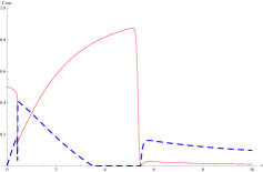
Figure 7: The three concurrences $C_{12}=C_{23}$ (dashed blue line) and $C_{13}$ (solid red line) vs $x$. Abrupt changes are very well visible around $x=0.5$ and $x=5.5$, where the negativity exhibits the same feature. For $x=1$ the three concurrences assume the same value ($\approx 0.33$).

Figure 8 shows the complete dependence of $\mathcal{N}_{123}$ on temperature and coupling parameter, for $x=3$. We observed (by performing other plots, which we are not reporting here) that the qualitative behavior of $\mathcal{N}_{123}$ is independent on the specific value of $x$, provided it is neither too small nor too big. It is quite evident that the trend with respect to temperature is the usual one. At low temperature the dependence of $\mathcal{N}_{123}$ on $c$ exhibits only the step trend due to level crossings. The highest step involves the energy levels $E_{4}^{-}(c,x=3)=-c\sqrt{11}-\omega_{0}$ and $E_{2}^{-}(c,x=3)=-\left(3+\sqrt{17}\right)c/2$ (see Appendix A), and it is quite easy to find that the crossing occurs at $c_{t}\approx 4.08\omega_{0}$ where $E_{4}^{-}=E_{2}^{-}$ while $E_{4}^{-}<E_{2}^{-}$ for $c<c_{t}$ and $E_{2}^{-}<E_{4}^{-}$ for $c>c_{t}$.

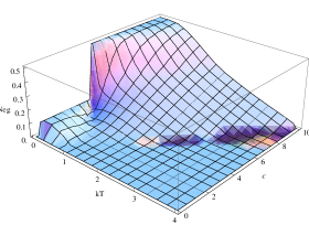
Figure 8: Negativity $\mathcal{N}_{123}$ as a functions of temperature ($k_{B}T$) and coupling parameter ($c$) at $x=3$, for the inhomogeneous model of type A, both $k_{B}T$ and $c$ are in units of $\omega_{0}$. With respect to $c$, at low temperature, there are abrupt changes traceable back to the occurrence of level crossings.

To conclude the analysis of the inhomogeneous model of type A, in Fig. 9 we have plotted the complete dependence of $\mathcal{N}_{123}$ on coupling and inhomogeneity parameters, fixing the value of temperature at $k_{B}T=0.01\omega_{0}$. The dependence on the coupling parameter is qualitatively the same as for the previous case (see Fig. 8). Indeed, we observe a step trend caused by a level crossing between the two lowest energy levels. As a function of $x$, $\mathcal{N}_{123}$ exhibits both smooth decreasing, due to increasing separability of spins $1$ and $3$, and fast variations traceable back to a level crossing amongst the two lowest energy levels $E_{2}^{-}$ and $E_{4}^{-}$. In fact, we verified that the big step observed in Fig. 9 corresponds to the locus of points of the plane $(c,x)$ in which the two lowest levels have the same energy. Thanks to the simple form of the eigenvalues of our model, one can find a simple analytical expression of this curve:

$$c(x)=\frac{x^{2}+4+\alpha(x)}{4x}+\frac{1}{2}\sqrt{\frac{x^{2}+5+\alpha(x)}{2}}\quad,$$ (13)

where $\alpha(x)$ is

$$\alpha(x)=\sqrt{16+10x^{2}+x^{4}}\quad.$$ (14)

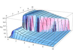
Figure 9: Negativity $\mathcal{N}_{123}$, at low temperature ($k_{B}T=0.01\omega_{0}$), versus coupling parameter ($c$, in units of $\omega_{0}$) and inhomogeneity parameter ($x$), for the inhomogeneous model of type A. Both smooth decreasing and fast variations occur with respect to $x$. Dependence on $c$ exhibits a stepwise behavior.

IV.2 Model with inhomogeneity of type B

The second type of inhomogeneity we decided to study is characterized by the coupling constants $c_{1}=c$, $c_{2}=c\>x$ and $c_{3}=c\>x^{2}$. Also for this model we have considered the dependence on $T$, $c$ and $x$. Surprisingly, what we have found is that the behavior of negativity in the presence of inhomogeneity of type B is not different from what we have found in the presence of inhomogeneity of type A. The diminishing for increasing temperature, the abrupt changes at low temperature in connection with level crossings and the presence of a maximum for $x\not=1$ are all present also in this model of inhomogeneity. Since for type B we do not have an explicit analytical diagonalization of the Hamiltonian, we also miss an analytical expression of the state of the system in the nearby of the maximum. In fact, we have only numerical results, according to which, for example, for $T=0.01\,\omega_{0}/k_{B}$ and $c=6\,\omega_{0}$ the maximum of negativity occurs at $x=x_{M}\approx 1.91$, where the ground state of the system is approximately: $\left|\Psi_{M}^{(B)}\right\rangle=0.292\left(\left|1100\right\rangle-\left|0011\right\rangle\right)+0.471\left(\left|1001\right\rangle-\left|0110\right\rangle\right)+0.439\left(\left|1010\right\rangle-\left|0101\right\rangle\right)$.

V Conclusions

In this paper we have analyzed the thermal correlations in a spin-star system consisting of a central spin interacting with three outer ones, all immersed in a magnetic field. In the absence of a tripartite entanglement measure, we have decided to exploit the tripartite negativity, which is at least able to put in evidence the lack of separability and simple bi-separability of a mixed quantum state of a tripartite system.

We started from considering the homogeneous model in which the three peripheral spins interact in the same way with the central one, showing the appearance of a significant degree of inseparability revealed by a non vanishing tripartite negativity ${\cal N}_{123}$. Typical behavior of thermal correlations reflects the behavior of ${\cal N}_{123}$, which decreases to zero-value as temperature increases and, instead, exhibits both appreciable values and abrupt changes at very low temperature. These occurrences show in a very clear way the role of thermal entanglement mediator played by the central spin. Further we have considered the presence of inhomogeneity, meant as differences in the coupling constants between the outer spins and the central one, focusing on two special cases. In the first case (inhomogeneity of type A) two spins interact in the same way with the central one and the third has a different coupling constant. In the second case (inhomogeneity of type B) all the three outer spins are characterized by different coupling strengths. Though some differences are visible, the qualitative behaviors of ${\cal N}_{123}$ are quite similar for the two inhomogeneous models and even for the homogeneous one. This suggests the idea that the thermal quantum correlations mediated by the central spin are not very much damaged by a certain lack of homogeneity that could characterize a more realistic situation, provided the degree of inhomogeneity is not high.

A remarkable point is that we have singled out the presence of maxima of tripartite negativity corresponding to inhomogeneous models, i.e. for the values of the inhomogeneous parameter quite larger than $1$. Though the differences between a maximum value of negativity and its values in the nearby (even up to the homogeneous case, i.e. up to $x=1$) is not very big, we think that it is conceptually important the fact that a higher degree of symmetry in the system does not guarantee a higher degree of correlations between all its parts.

Another important point is that we have found some regions of the parameter space where it happens that two concurrences, say ${\cal C}_{12}$ and ${\cal C}_{23}$, are vanishing, meaning that there is no entanglement between $1$ and $2$ and between $2$ and $3$, while the relevant negativity ${\cal N}_{2-13}$ is non-vanishing, meaning that there is a correlation between $2$ and the couple made of $1$ and $3$. This fact points out in a very transparent way the different meanings of concurrence and negativity.

Appendix A

In this appendix we give eigenvalues and eigenvectors of the Hamiltonian of the inhomogeneous model of type A ($c_{1}=c$, $c_{2}=c\>x$, $c_{3}=c$), as functions of $x>0$, $c>0$, $\omega_{0}$. The special case $x=1$ gives the solutions for the homogeneous model.

$$\begin{array}[]{ll}\textrm{Energies}&\textrm{Eigenstates}\\ E_{1}^{\pm}=\pm c\>x\,,&\left|\Psi_{1}^{\pm}\right\rangle=\frac{1}{2}\left[\left(\left|0011\right\rangle\pm\left|1100\right\rangle\right)-\left(\left|0110\right\rangle\pm\left|1001\right\rangle\right)\right]\,,\\ E_{2}^{\pm}=\pm\frac{c}{2}\left[x+\left(8+x^{2}\right)^{\frac{1}{2}}\right]\,,&\left|\Psi_{2}^{\pm}\right\rangle=\frac{1}{K_{1}}\>\left[\left(\left|0011\right\rangle\pm\left|1100\right\rangle\right)+\left(\left|0110\right\rangle\pm\left|1001\right\rangle\right)\right.\\ &\left.+\frac{\sqrt{8+x^{2}}-x}{2}\left(\left|0101\right\rangle\pm\left|1010\right\rangle\right)\right]\,,\\ E_{3}^{\pm}=\pm\frac{c}{2}\left[x-\left(8+x^{2}\right)^{\frac{1}{2}}\right]\,,&\left|\Psi_{3}^{\pm}\right\rangle=\frac{1}{K_{1}}\>\left[\left(\left|0011\right\rangle\pm\left|1100\right\rangle\right)+\left(\left|0110\right\rangle\pm\left|1001\right\rangle\right)\right.\\ &\left.-\frac{\sqrt{8+x^{2}}+x}{2}\left(\left|0101\right\rangle\pm\left|1010\right\rangle\right)\right]\,,\\ E_{4}^{\pm}=\pm\left[c\left(2+x^{2}\right)^{\frac{1}{2}}+\omega_{0}\right]\,,&\left|\Psi_{4}^{\pm}\right\rangle=\frac{1}{K_{2}}\left[\sqrt{2+x^{2}}\left|0111\right\rangle\right.\\ &\left.\pm\left(\left|1011\right\rangle+x\left|1101\right\rangle+\left|1110\right\rangle\right)\right]\,,\\ E_{5}^{\pm}=\pm\left[c\left(2+x^{2}\right)^{\frac{1}{2}}-\omega_{0}\right]\,,&\left|\Psi_{5}^{\pm}\right\rangle=\frac{1}{K_{2}}\left[\left(\left|0100\right\rangle+x\left|0010\right\rangle+\left|0001\right\rangle\right)\right.\\ &\left.\pm\sqrt{\left(2+x^{2}\right)}\left|1000\right\rangle\right]\,,\\ E_{6}=-\omega_{0}\,,&\left|\Psi_{6}^{A}\right\rangle=\frac{1}{K_{3}}\left[\frac{1}{x}\left|0001\right\rangle+\left|0010\right\rangle-\left(\frac{1}{x}+x\right)\left|0100\right\rangle\right]\,,\\ &\left|\Psi_{6}^{B}\right\rangle=\frac{1}{\sqrt{1+x^{2}}}\left(\left|0010\right\rangle-x\left|0001\right\rangle\right)\,,\\ E_{7}=\omega_{0}\,,&\left|\Psi_{7}^{A}\right\rangle=\frac{1}{K_{3}}\left[\frac{1}{x}\left|1011\right\rangle+\left|1101\right\rangle-\left(\frac{1}{x}+x\right)\left|1110\right\rangle\right]\,,\\ &\left|\Psi_{7}^{B}\right\rangle=\frac{1}{\sqrt{1+x^{2}}}\left(\left|1101\right\rangle-x\left|1011\right\rangle\right)\,,\\ E_{8}=-2\omega_{0}\,,&\left|\Psi_{8}\right\rangle=\left|0000\right\rangle\,,\\ E_{9}=2\omega_{0}\,,&\left|\Psi_{9}\right\rangle=\left|1111\right\rangle\,,\\ \end{array}$$

where $K_{1}$, $K_{2}$ and $K_{3}$ are:

$${K_{1}}^{2}=4+2\left(\frac{\sqrt{8+x^{2}}-x}{2}\right)^{2}\,,$$

$${K_{2}}^{2}=2\left(2+x^{2}\right)\,,$$

$${K_{3}}^{2}=\frac{2}{x^{2}}+3+x^{2}\,.$$

References

- (1) Arnesen M C, Bose S, Vedral V 2001 Phys. Rev. Lett. 87 017901.
- (2) Osterloh A et al 2002 Nature 416, 608.
- (3) Osborne T J and Nielsen M A 2002 Phys. Rev. A 66 032110
- (4) Vedral V 2004 New. J. Phys. 6 102.
- (5) Wiesniak M, Vedral V and Brukner C 2005 New J. Phys. 7 258.
- (6) Vedral V 2008 Nature 453, 1004.
- (7) Shou-Shu Gong and Gang Su 2009 Phys. Rev. A 80 012323.
- (8) Hao Wang, Sanqiu Liu, and Jizhou He 2009 Phys. Rev. E 79 041113.
- (9) Amit Kumar Pal and Indrani Bose 2010 J. Phys.: Cond. Matt. 22 016004.
- (10) Werlang T and Rigolin G 2010 Phys. Rev. A 81 044101
- (11) Souza A M et al 2009 Phys. Rev. B 79 054408.
- (12) Yue Zhou et al 2009 Europhys. Lett. 86 50004.
- (13) Makhlin Y, Schoen G, Shnirman A 1999, Nature 398, 305
- (14) Cirac J I, Zoller P 2000 Nature 404 579
- (15) Keane B E 1998 Nature 393 133
- (16) Hutton A, Bose S 2004 Phys. Rev. A 69 042312.
- (17) Wan-Li Y, Hua W, Mang F, Jun-Hong A 2009 Chinese Phys. B 18 3677.
- (18) Wootters W K 1998 Phys. Rev. Lett. 80 2245.
- (19) For a review on entanglement in multipartite systems, see: Amico L, Fazio R, Osterloh A and Vedral V 2008 Rev. Mod. Phys. 80 517.
- (20) Sabin C, Garcia-Alcaine G 2008 Eur. Phys. J. D 48, 435.
- (21) Coffman V, Kundu J, Wootters W K 2000 Phys. Rev. A 61 052306.
- (22) Wong A and Christensen N 2001 Phys. Rev. A 63 044301.
- (23) Meyer D A and Wallach N R 2002 J. Math. Phys. 43 4273
- (24) Facchi P, Florio G, Marzolino U, Parisi G and Pascazio S 2009 J. Phys. A: Math. Theor. 42 055304
- (25) Horodecki M, Horodecki P and Horodecki R, 1996 Phys. Lett. A 223 1; Terhal B, Phys. lett. A 2000 271 319.
- (26) Lin Chen and Yi-Xin Chen 2007 Phys. Rev. A 76, 022330.
- (27) Wiesiak M, Vedral V, Brukner C 2005 New J. Phys. 7 258.
- (28) Brandão Fernando G S L 2005, Phys. Rev. A 72 022310.
- (29) Coffman V, Kund J, Wootters W K 2000 Phys. Rev. A 61 052306.
- (30) Jung E, Park D, Son J 2009 Phys. Rev. A 80 010301(R).
- (31) Zyczkowski K, Horodecki P, Sanpera A, Lewenstein M, 1998, Phys. Rev. A 58 883.
- (32) Vidal G, Werner R F 2002 Phys. Rev. A 65 032314.