Improving quantum entanglement through single-qubit operations

Abstract

We show that the entanglement of a $2\times 2$ bipartite state can be improved and maximized probabilistically through single-qubit operations only. An experiment is proposed and it is numerically simulated.

Introduction.— Quantum entanglement plays a central role in quantum information and also in the foundations of quantum physics. Thus, it has been extensively studied (see, e.g., amico ; horodecki ; pv ; Yutin ; sci ; nor ). One important topic here is how to improve quantum entanglement of a bipartite quantum state bennett . As is well known, quantum entanglement can be improved through entanglement purification bennett where a bipartite state is first transformed to a Werner state and then two-qubit operations at each sides are needed to improve the quantum entanglement probabilistically.

In this letter, we shall present a theorem (Theorem 2) to maximize the entanglement of a two-qubit mixed state through single-qubit operations only. The theorem can be used to efficiently improve the quantum entanglement of a mixed state without the difficult 2-qubit operations. Explicitly, given a two-qubit mixed state $\rho_{\textrm{in}}=\rho_{12}$, by taking local (non-trace-preserving Italy ) maps on qubit 1 and qubit 2 separately, what is the maximally achievable entanglement of the normalized outcome state, and what are the specific maps needed on each qubits.

To make a clear picture of our work we consider the following example with a pure state $\rho_{\textrm{in}}=|\chi\rangle\langle\chi|$ and $|\chi\rangle=a|00\rangle+b|11\rangle$ first. Take the following specific non-trace-preserving map on the first qubit:

$$\varepsilon\otimes I(\rho_{{\rm in}})=\hat{M}(\tilde{a},\tilde{b})\otimes I\cdot\rho_{{\rm in}}\cdot\hat{M}(\tilde{a},\tilde{b})\otimes I,$$ (1)

where $\hat{M}(\tilde{a},\tilde{b})=\tilde{a}|0\rangle\langle 0|+\tilde{b}|1\rangle\langle 1|$, and $|\tilde{a}|^{2}+|\tilde{b}|^{2}=1$. We have

$$\varepsilon\otimes I(\rho_{{\rm in}})=\gamma|\chi^{\prime}\rangle\langle\chi^{\prime}|,$$ (2)

and $\gamma=\sqrt{|a\tilde{a}|^{2}+|b\tilde{b}|^{2}}$, $|\chi^{\prime}\rangle=\frac{a\tilde{a}}{\gamma}|00\rangle+\frac{b\tilde{b}}{\gamma}|11\rangle$. The entanglement concurrence of the outcome state is

$$C(|\chi^{\prime}\rangle\langle\chi^{\prime}|)=\frac{2|a\tilde{a}b\tilde{b}|}{|a\tilde{a}|^{2}+|b\tilde{b}|^{2}}.$$ (3)

Setting $|\tilde{a}|=|b|$ and $|\tilde{b}|=|a|$, we shall obtain the maximum output entangled state $|\phi^{+}\rangle=\frac{1}{\sqrt{2}}(|00\rangle+|11\rangle)$ state (up to a normalization factor). Physically, the map $\hat{M}(\tilde{a},\tilde{b})$ can be easily realized. For example qip , one can use a polarization-dependent attenuator, with transmittance proportional to $\tilde{a}$ for a horizontally polarized photon (state $|0\rangle$) and transmittance proportional to $\tilde{b}$ for a vertically polarized photon (state $|1\rangle$). Once we find a photon at the outcome port of the attenuator, the initial state $|\chi\rangle\langle\chi|$ has been mapped to the outcome state $|\chi^{\prime}\rangle\langle\chi^{\prime}|$.

Outline of our work.— Our goal is to look for the largest achievable entanglement through local operations, i.e., among all physical maps $\varepsilon\otimes\varepsilon^{\prime}:\rho_{\textrm{out}}=\varepsilon\otimes\varepsilon^{\prime}(\rho_{\textrm{in}})$, which map gives out the largest entanglement of the outcome state $\rho_{\textrm{out}}$. Most generally, any local map $\varepsilon\otimes\varepsilon^{\prime}$ can be represented in the form of Kruss operators Italy :

$$\rho_{\textrm{out}}=\sum_{i}{\Gamma_{i}\otimes\Gamma_{i}^{\prime}\cdot\rho_{\textrm{in}}\cdot(\Gamma_{i}\otimes\Gamma_{i}^{\prime})^{\dagger}}=\sum_{i}p_{i}\rho_{i},$$ (4)

where $p_{i}\rho_{i}=\Gamma_{i}\otimes\Gamma_{i}^{\prime}\rho_{\textrm{in}}(\Gamma_{i}\otimes\Gamma_{i}^{\prime})^{\dagger}$. Denote $C(\rho)$ as the entanglement concurrence Wooters of state $\rho$. Suppose $C(\rho_{m})$ is the largest among all $\{C(\rho_{i})\}$. Obviously,

$$C(\rho_{\textrm{out}})\;\leq\;\sum_{i}p_{i}C(\rho_{i})\;\leq\;C(\rho_{m}).$$ (5)

Therefore, to find the largest entanglement concurrence of the outcome state among all local maps, we only need to seek it in the following special class of maps: $\rho_{\textrm{out}}=\mathcal{Q}\otimes\mathcal{Q^{\prime}}\rho_{\textrm{in}}(\mathcal{Q}\otimes\mathcal{Q^{\prime}})^{\dagger}$ where $\mathcal{Q},\mathcal{Q}^{\prime}$ are $2\times 2$ positive matrices. According to the singular-value decomposition, the positive matrix $\mathcal{Q}$($\mathcal{Q^{\prime}}$) can be decomposed into $\mathcal{Q}=U_{1}DU$($\mathcal{Q^{\prime}}=U_{1}^{\prime}D^{\prime}U^{\prime}$) where $U_{1},U$($U_{1}^{\prime},U^{\prime}$) are unitary matrices and $D$($D^{\prime}$) is a positive-definite diagonal matrix. Since a unitary transformation plays no role in the entanglement, we only need to consider the positive matrices in the form of $DU$ ($D^{\prime}U^{\prime}$).

As shown in Lemma 2, any two-qubit state $\rho_{\textrm{in}}$ can be generated from the maximally-entangled state $|\phi^{+}\rangle$ acted by a one-sided map $I\otimes\varepsilon^{\prime}$, i.e., $\rho_{\textrm{in}}=I\otimes\varepsilon^{\prime}(|\phi^{+}\rangle\langle\phi^{+}|)$. Therefore, we can start with entanglement evolution and maximization under non-trace-preserving one-sided maps and then apply the result to the general problem of improving and maximizing quantum entanglement through single-qubit operations.

Entanglement evolution and maximization under non-trace-preserving maps.— A non-trace-preserving one-sided map $I\otimes\varepsilon^{\prime}$ is fully characterized by $\rho_{\varepsilon^{\prime}}=I\otimes\varepsilon^{\prime}(|\phi^{+}\rangle\langle\phi^{+}|)$ liusky . We assume

$$I\otimes\varepsilon^{\prime}(|\phi^{+}\rangle\langle\phi^{+}|)=f\rho_{\varepsilon^{\prime}},\;I\otimes\varepsilon^{\prime}(|\psi\rangle\langle\psi|)=f^{\prime}\rho_{\psi}\;,$$ (6)

where $f={\rm tr}\left[I\otimes\varepsilon^{\prime}(|\phi^{+}\rangle\langle\phi^{+}|)\right]$, $f^{\prime}={\rm tr}\left[I\otimes\varepsilon^{\prime}(|\psi\rangle\langle\psi|)\right]$.

A $2\times 2$ pure state $|\chi\rangle=a|00\rangle+b|11\rangle$ can be rewritten in the form $|\chi\rangle\langle\chi|=2\hat{M}(a,b)\otimes I(|\phi^{+}\rangle\langle\phi^{+}|)\hat{M}(a,b)\otimes I$. From Eq. (6) we have $I\otimes\varepsilon^{\prime}(|\chi\rangle\langle\chi|)=2f\hat{M}(a,b)\otimes I\rho_{\varepsilon^{\prime}}\hat{M}(a,b)\otimes I=f^{\prime}\rho_{\chi}$. We emphasize here that even though $\rho_{\varepsilon^{\prime}}$ is normalized, the operator $2\hat{M}(a,b)\otimes I\rho_{\varepsilon^{\prime}}\hat{M}(a,b)\otimes I$ is not necessarily normalized. Define the following function $C$ of an arbitrary non-negative definite $4\times 4$ matrix (operator) $N$

$$C(N)=\rm{max}\{0,\sqrt{\xi}_{1}-\sqrt{\xi}_{2}-\sqrt{\xi}_{3}-\sqrt{\xi}_{4}\},$$ (7)

where $\{\xi_{i}\}$ are the eigenvalues of $N\cdot\tilde{N}$, in descending order, with $\tilde{N}=\sigma_{y}\otimes\sigma_{y}N^{*}\sigma_{y}\otimes\sigma_{y}$, and $N^{*}$ is the complex conjugate of $N$. If $N$ is a density matrix of a $2\times 2$ system, $C(N)$ is just the entanglement concurrence of the system Wooters . With this definition of $C$, we can summarize the major result, equation (5) in Ref. 1 as:
Lemma 1. Given any density matrix $\rho_{\varepsilon^{\prime}}$, if $N=2\hat{M}(a,b)\otimes I\rho_{\varepsilon^{\prime}}\hat{M}^{\dagger}(a,b)\otimes I$, then

$$C(N)\;=\;C(|\chi\rangle\langle\chi|)\cdot C(\rho_{\varepsilon^{\prime}})\;=\;2|ab|C(\rho_{\varepsilon^{\prime}}).$$ (8)

However, this is not the entanglement concurrence of $\rho_{\chi}$ because $N$ is not necessarily normalized, even though $\rho_{\varepsilon^{\prime}}$ is. Now denote $N=g\rho_{\chi}$, and $g={\rm tr}N$. According to the definition of $C$ and $\rho_{\psi}$ in Eq. (6),

$$C(\rho_{\chi})\ =\ C(N)/g\ =\ 2|ab|C(\rho_{\varepsilon^{\prime}})/g$$ (9)

where $g={\rm tr}N=2{\rm tr}[\hat{M}(a,b)\otimes I\rho_{\varepsilon^{\prime}}\hat{M}^{\dagger}(a,b)\otimes I]$. To avoid meaningless results, we assume $C(\rho_{\varepsilon}^{\prime})>0$ throughout this paper. Assume that the density matrix of the first qubit of $\rho_{\varepsilon^{\prime}}$ is $\rho_{0}=\rm{tr}_{2}\rho_{\varepsilon^{\prime}}=\left(\begin{array}[]{cc}c_{1}&\alpha\\ \alpha^{*}&c_{2}\end{array}\right)=K_{0}$, where $\rm{tr}_{2}$ is the partial trace over the subspace of the second qubit and $c_{1}=\langle 0|{\rm tr}_{2}\rho_{\varepsilon^{\prime}}|0\rangle,\;c_{2}=\langle 1|{\rm tr}_{2}\rho_{\varepsilon^{\prime}}|1\rangle.$ Consequently,

$$g=2{\rm tr}[M(a,b)\rho_{0}M^{\dagger}(a,b)]=2|a|^{2}c_{1}+2|b|^{2}c_{2}.$$ (10)

Therefore, the value of output entanglement

$$C(\rho_{\chi})=\frac{2|ab|C(\rho_{\varepsilon^{\prime}})}{(|a|^{2}c_{1}+|b|^{2}c_{2})},$$ (11)

is maximized when $|a|=\sqrt{c_{2}},\;|b|=\sqrt{c_{1}}$, with the maximum value

$$C(\rho_{\chi})=\frac{C(\rho_{\varepsilon^{\prime}})}{2\sqrt{c_{1}c_{2}}}.$$ (12)

More generally, the initial pure state can be

$$|\psi\rangle=I\otimes U|\chi\rangle=\sqrt{2}\hat{M}(a,b)\otimes U|\phi\rangle,$$ (13)

where $U$ is an arbitrary unitary operator. Given the fact that $U^{*}\otimes U|\phi^{+}\rangle=|\phi^{+}\rangle$ for any unitary $U$, we have

$$\sqrt{2}\hat{M}(a,b)\otimes U|\phi^{+}\rangle=\sqrt{2}\hat{M}(a,b)U^{T}\otimes I|\phi^{+}\rangle.$$ (14)

In such a case, we obtain

$$C(\rho_{\psi})=2|ab|\cdot C(\rho_{\varepsilon^{\prime}})/g^{\prime}$$ (15)

and $g^{\prime}={\rm tr}[\hat{M}(a,b)U^{T}\otimes I\rho_{\varepsilon^{\prime}}U^{*}\hat{M}(a,b)\otimes I]$. To maximize $C(\rho_{\psi})$, we first fix $U$ and maximize it with $a,b$. Assume $U^{T}K_{0}U^{*}=\left(\begin{array}[]{cc}c_{1}^{\prime}&\alpha^{\prime}\\ \alpha^{\prime*}&c_{2}^{\prime}\end{array}\right).$ The largest value for $C(\rho_{\psi})$ is ${C(\rho_{\varepsilon^{\prime}})}/{2\sqrt{c_{1}^{\prime}c_{2}^{\prime}}}$, as shown already. To maximize the value over all $U$, we only need to minimize $c_{1}^{\prime}c_{2}^{\prime}$. Since $U$ is unitary, $\det(U^{T}K_{0}U^{*})=\det K_{0}$. Therefore $c_{1}^{\prime}c_{2}^{\prime}=\det K_{0}+|\alpha^{\prime}|^{2}$, which is minimized when $\alpha^{\prime}=0$. Namely, $C(\rho_{\psi})$ is maximized when $U^{T}K_{0}U^{*}$ is diagonalized and $\sqrt{a}=c_{2}^{\prime},~{}\sqrt{b}=c_{1}^{\prime}$, i.e., $\hat{M}(a,b)U^{T}\left({\rm tr}_{2}\rho_{\varepsilon^{\prime}}\right)U^{*}\hat{M}(a,b)={\rm diag}[1/2,1/2]$. We obtain
Theorem 1. Denote $\mathcal{Q}$ to be a $2\times 2$ positive-definite matrix. Given the inseparable two-qubit density matrix $\rho_{\textrm{in}}=\rho_{\varepsilon^{\prime}}=I\otimes\varepsilon^{\prime}(|\phi^{+}\rangle\langle\phi^{+}|)$, the entanglement of the normalized density matrix $\rho_{1}=\mathcal{Q}\otimes I\rho_{\textrm{in}}(\mathcal{Q}\otimes I)^{\dagger}$ maximizes when $\mathcal{Q}\left({\rm tr_{2}}\rho_{\textrm{in}}\right){\mathcal{Q}}^{\dagger}={\rm diag}[1/2,1/2]$ and the entanglement concurrence is:

$$C_{M}=\frac{C(\rho_{\varepsilon^{\prime}})}{2\sqrt{\det\left[{\rm tr}_{2}\rho_{\varepsilon^{\prime}}\right]}}.$$ (16)

Improving and maximizing quantum entanglement through single-qubit operations.— To apply our theorem, we need the following lemma:

Lemma 2. Given any $2\times 2$ bipartite mixed state $\rho_{12}$, there exists a map $\varepsilon^{\prime}$ such that $\rho_{\textrm{in}}=I\otimes\varepsilon^{\prime}(|\phi^{+}\rangle\langle\phi^{+}|)$.

Note that map $\varepsilon^{\prime}$ here is in general non-trace-preserving. Since any two-qubit density matrix $\rho_{\textrm{in}}$ can be decomposed into the mixture of a few pure states, say $\rho_{\textrm{in}}=\sum_{i}\lambda_{i}|\psi_{i}\rangle\langle\psi_{i}|$. Obviously, for any bipartite pure state $|\psi_{i}\rangle$, there always exists a positive operator $\hat{M}_{i}^{\prime}$ such that $|\psi_{i}\rangle=I\otimes\hat{M}_{i}^{\prime}|\phi^{+}\rangle$. Therefore, we have $\rho_{\textrm{in}}=\sum_{i}\lambda_{i}I\otimes\hat{M}_{i}^{\prime}|\phi^{+}\rangle\langle\phi^{+}|I\otimes\hat{M}_{i}^{\prime\dagger}$. Denoting $I\otimes\varepsilon^{\prime}(|\phi^{+}\rangle\langle\phi^{+}|)=\sum_{i}I\otimes\sqrt{\lambda}_{i}\hat{M}_{i}^{\prime}|\phi^{+}\rangle\langle\phi^{+}|I\otimes\sqrt{\lambda}_{i}\hat{M}_{i}^{\prime\dagger}$ completes the proof.

With Theorem 1 and Lemma 2, we can improve the quantum entanglement of any 2-qubit state $\rho_{\textrm{in}}$ (here and after, the 2-qibit states are normalized) step by step, with single-qubit operations only. Denote $K_{1}={\rm tr}_{2}\rho_{\textrm{in}}$, if $\det K_{1}<1/4$, we construct $\hat{M}_{1}(\tilde{a}_{1},\tilde{b}_{1})$ and local unitary $U_{1}$ such that $\hat{M}_{1}U_{1}K_{1}U_{1}^{\dagger}\hat{M}_{1}^{\dagger}={\rm diag[1/2,1/2]}$. The local operation on qubit 1 transforms state $\rho_{\textrm{in}}$ into the outcome state $\rho_{1}=\hat{M}_{1}U_{1}\otimes I\rho_{\textrm{in}}U_{1}^{\dagger}\hat{M}_{1}^{\dagger}\otimes I$. According to Theorem 1, the entanglement concurrence of the outcome state is $C(\rho_{1})=C(\rho_{\textrm{in}})/(2\sqrt{\det{K_{1}}})>C(\rho_{\textrm{in}})$. The normalized density matrix of qubit 1 is $\textrm{tr}_{2}\rho_{1}={\rm diag}[1/2,1/2]$ now, but in general the normalized density operator of qubit 2 is not ${\rm diag}[1/2,1/2]$ now. Using Lemma 2, we know $\rho_{1}$ can be written in the form of $\rho_{1}=\varepsilon\otimes I(|\phi^{+}\rangle\langle\phi^{+}|)$. We can now apply Theorem 1 again to further improve the quantum entanglement through operation on qubit 2. Denote $K_{1}^{\prime}={\rm{tr}_{1}}\rho_{1}$. If $\det(K_{1}^{\prime})<1/4$, we construct new operators $\hat{M}_{1}^{\prime}$ and $U_{1}^{\prime}$ such that the density matrix of qubit 2 is ${\rm diag}[1/2,1/2]$ after the operation, i.e., $\hat{M}_{1}^{\prime}U_{1}^{\prime}({\rm tr}_{1}\rho_{1})U_{1}^{{}^{\prime}\dagger}\hat{M}_{1}^{{}^{\prime}\dagger}={\rm diag}[1/2,1/2]$. The operation on qubit 2 leads to a new outcome state $\rho_{1}^{\prime}=I\otimes\hat{M}_{1}^{\prime}U_{1}^{\prime}\rho_{1}I\otimes U_{1}^{{}^{\prime}\dagger}\hat{M}_{1}^{{}^{\prime}\dagger}$. The operation on qubit 2 improves the entanglement concurrence to $C(\rho_{1}^{\prime})=C(\rho_{1})/(2\sqrt{\det K_{1}^{\prime}})>C(\rho_{1})$. After the non-trace-preserving operation above on qubit 2, we have $K_{1}^{\prime}=\textrm{tr}_{1}\rho_{1}^{\prime}={\rm diag}[1/2,1/2]$, but in general the density matrix of qubit 1 is not ${\rm diag}[1/2,1/2]$, i.e. $K_{2}=\textrm{tr}_{2}\rho_{1}^{\prime}\not={\rm diag}[1/2,1/2]$ now. We can construct new operators $\hat{M}_{2}$ and $U_{2}$ to improve the entanglement of $\rho_{1}^{\prime}$. The process will continue step by step until the determinant of two reduced density matrices are all equal to $1/4$ after many steps of iterations. Since the entanglement concurrence of a two-qubit state can never be greater than 1 and the entanglement always increases during the iteration process above, there must exist a limit value of the entanglement in the process say, after many steps of iterations, the process gives out the largest entanglement concurrence. This also means that after many steps of iterations, the process always produces a two-qubit state where the reduced density matrices of each qubit are ${\rm diag}[1/2,1/2]$ simultaneously. Therefore the process that transfers the reduced density matrix of qubit 1 and the reduced density matrix of qubit 2 into ${\rm diag}[1/2,1/2]$ simultaneously always exists and can be written in the following form:

$$\rho_{f}=\prod_{k=1}^{\infty}{\hat{M}_{k}U_{k}\otimes\hat{M}_{k}^{\prime}U_{k}^{\prime}}\cdot\rho_{\textrm{in}}\cdot\prod_{k=1}^{\infty}{U_{k}^{\dagger}\hat{M}_{k}^{\dagger}\otimes U_{k}^{{}^{\prime}\dagger}\hat{M}_{k}^{{}^{\prime}\dagger}}.$$ (17)

At the same time, the final state $\rho_{f}$ satisfies the following condition:

$${\rm tr_{1}}\rho_{f}={\rm tr_{2}}\rho_{f}=I/2.$$ (18)

As an example, consider the imperfect entangled state

$$\tilde{\rho}=0.1|\varphi^{\prime}\rangle\langle\varphi^{\prime}|+0.12|\varphi^{\prime\prime}\rangle\langle\varphi^{\prime\prime}|+0.78|\phi^{+}\rangle\langle\phi^{+}|,$$ (19)

where $|\varphi^{\prime}\rangle=\hat{R}(\theta_{1})\otimes I|00\rangle$, $|\varphi^{\prime\prime}\rangle=\hat{R}(\theta_{2})\otimes I|11\rangle$ with $\theta_{1}=\pi/5,\theta_{2}=-3\pi/10$ and $\hat{R}(\theta)=\left(\begin{array}[]{cc}\cos\theta&\sin\theta\\ \sin\theta&-\cos\theta\end{array}\right)$. The entanglement increase through 7 steps of iteration is shown in Fig. 1.

Figure 1: (color online) The concurrence $C$ versus number of iterations of single-qubit operation.

The remaining task is to show that, starting from the same state $\rho_{\textrm{in}}$, all final states satisfying Eq. (18) have the same value for entanglement concurrence.
Lemma 3. If state $\rho_{f}$ satisfies Eq. (18), then state $\rho_{f}^{\prime}=U\otimes U^{\prime}\rho_{f}U^{\dagger}\otimes{U^{\prime}}^{\dagger}$ also satisfies Eq. (18). Here $U,U^{\prime}$ are any two unitary operators.

This conclusion is obvious since a unity density operator remains to be unity after any local unitary transformation.

Assume we have two different final states $\rho_{u},\rho_{v}$ obtained by using different processes from the same initial state, and they satisfy Eq. (18). Suppose

$$\rho_{u}=\prod_{k=1}^{\infty}{\hat{\mathcal{M}}_{k}\mathcal{U}_{k}\otimes\hat{\mathcal{M}}_{k}^{\prime}\mathcal{U}_{k}^{\prime}}\cdot\rho_{\textrm{in}}\cdot\prod_{k=1}^{\infty}{\mathcal{U}_{k}^{\dagger}\hat{\mathcal{M}}_{k}^{\dagger}\otimes\mathcal{U}_{k}^{{}^{\prime}\dagger}\hat{\mathcal{M}}_{k}^{{}^{\prime}\dagger}},$$

$$\rho_{v}=\prod_{k=1}^{\infty}{\hat{\mathcal{N}}_{k}\mathcal{V}_{k}\otimes\hat{\mathcal{N}}_{k}^{\prime}\mathcal{V}_{k}^{\prime}}\cdot\rho_{\textrm{in}}\cdot\prod_{k=1}^{\infty}{\mathcal{V}_{k}^{\dagger}\hat{\mathcal{N}}_{k}^{\dagger}\otimes\mathcal{V}_{k}^{{}^{\prime}\dagger}\hat{\mathcal{N}}_{k}^{{}^{\prime}\dagger}},$$

where $\hat{\mathcal{M}}_{k},\hat{\mathcal{M}}_{k}^{\prime},\hat{\mathcal{N}}_{k},\hat{\mathcal{N}}_{k}^{\prime}$ are projective operators and $\mathcal{U}_{k},\mathcal{U}_{k}^{\prime},\mathcal{V}_{k},\mathcal{V}_{k}^{\prime}$ are unitary operators. By using singular-value decomposition, We have

$$\rho_{v}=\tilde{\mathcal{W}}\mathcal{P}\mathcal{W}\otimes\tilde{\mathcal{W}}^{\prime}\mathcal{P}^{\prime}\mathcal{W}^{\prime}\cdot\rho_{u}\cdot\mathcal{W}^{\dagger}\mathcal{P}^{\dagger}\tilde{\mathcal{W}}^{\dagger}\otimes{\mathcal{W}^{\prime\dagger}}{\mathcal{P}^{\prime}}^{\dagger}{\tilde{\mathcal{W}}^{\prime\dagger}},$$ (20)

where $\tilde{\mathcal{W}},\mathcal{W},\tilde{\mathcal{W}}^{\prime},\mathcal{W}^{\prime}$ are unitary operators and $\mathcal{P},\mathcal{P}^{\prime}$ are projective operators defined in Eq. (1). Denote $\tilde{\rho}_{w}=\tilde{\mathcal{W}}^{\dagger}\otimes{\tilde{\mathcal{W}}^{\prime\dagger}}\rho_{v}\tilde{\mathcal{W}}\otimes\tilde{\mathcal{W}}^{\prime}$ and ${\rho}_{w}=\mathcal{W}\otimes\mathcal{W}^{\prime}\rho_{u}\mathcal{W}^{\dagger}\otimes{\mathcal{W}^{\prime\dagger}}$. We have

$$\tilde{\rho}_{w}=\mathcal{P}\otimes\mathcal{P}^{\prime}\rho_{w}\mathcal{P}^{\dagger}\otimes{\mathcal{P}^{\prime\dagger}}.$$ (21)

According to Lemma 3, we know that $\tilde{\rho}_{w},\rho_{w}$ satisfy Eq. (18). Thus $\mathcal{P}$ and $\mathcal{P}^{\prime}$ must be either identity or $\textrm{diag}[1,i]$. This indicates that $\mathcal{P}$ and $\mathcal{P}^{\prime}$ are unitary therefore the entanglement concurrence of $\tilde{\rho}_{w}$ and $\rho_{w}$ must be same. We now obtain the major result of this letter:
Theorem 2. Given any inseparable two-qubit initial state $\rho_{\textrm{in}}$, the entanglement concurrence can be improved through single-qubit operations provided that the reduced density matrix of any one qubit is not ${\rm diag[1/2,1/2]}$. Among all out-come states $\{\rho_{\textrm{out}}|\rho_{\textrm{out}}=\varepsilon\otimes\varepsilon^{\prime}(\rho_{\textrm{in}})\}$ through positive-definite local maps, the state $\rho_{\textrm{out}}=\mathcal{Q}\otimes\mathcal{Q^{\prime}}\rho_{\textrm{in}}\mathcal{Q}^{\dagger}\otimes\mathcal{Q^{\prime}}^{\dagger}$ has the largest entanglement concurrence if the density matrices of each qubit of the outcome state are $I/2$. The corresponding local maps at each side are simply positive-definite matrices $\mathcal{Q},\mathcal{Q^{\prime}}$ which can be constructed by Eq. (17), i.e., $\mathcal{Q}=\prod_{k=1}^{\infty}{\hat{M}_{k}U_{k}},\mathcal{Q^{\prime}}=\prod_{k=1}^{\infty}{\hat{M}_{k}^{\prime}U_{k}^{\prime}}$ where ${\hat{M}_{k}U_{k}}$ ($\hat{M}_{k}^{\prime}U_{k}^{\prime}$) diagonalize the state of the first (second) qubit into the form of $I/2$ at the corresponding step. Specifically, $\textrm{tr}_{2}[(\hat{M}_{k}U_{k}\otimes I)\rho_{k-1}^{\prime}(\hat{M}_{k}U_{k}\otimes I)^{\dagger}]=I/2$ and $\textrm{tr}_{1}[(I\otimes\hat{M}_{k}^{\prime}U_{k}^{\prime})\rho_{k}(I\otimes\hat{M}_{k}^{\prime}U_{k}^{\prime})^{\dagger}]=I/2$ where $\rho_{k}^{\prime}=\prod_{i=1}^{k}{(\hat{M}_{i}U_{i}\otimes\hat{M}_{i}^{\prime}U_{i}^{\prime})\rho_{\textrm{in}}(\hat{M}_{i}U_{i}\otimes\hat{M}_{i}^{\prime}U_{i}^{\prime})^{\dagger}}$ and $\rho_{k}=\hat{M}_{k}U_{k}\otimes I\rho_{k-1}^{\prime}(\hat{M}_{k}U_{k})^{\dagger}\otimes I$.
Remark: In the theorem, we have presented a mathematical way to construct $\mathcal{Q},\mathcal{Q^{\prime}}$ by iteration. We emphasize that, in applying our theorem in a real experiment, one can compute $\mathcal{Q},\mathcal{Q^{\prime}}$ and then realize the physical process in only one step.

Proposed experiment and numerical simulation.— We propose to test Theorem 2 with the initial state $\tilde{\rho}$ as defined in Eq. (19). With many iterations, we have $\mathcal{Q}=\prod_{k}\hat{M}_{k}U_{k}=\left(\begin{array}[]{cc}0.5875&-0.8090\\ 0.0130&0.0095\end{array}\right)$ and $\mathcal{Q^{\prime}}=\prod_{k}{\hat{M}^{\prime}}_{k}U_{k}^{\prime}=\left(\begin{array}[]{cc}0.0106&-0.0145\\ 0.8091&0.5874\end{array}\right)$. Then we find that the entanglement concurrence of the final state $\mathcal{Q}\otimes\mathcal{Q}^{\prime}\tilde{\rho}\mathcal{Q}^{\dagger}\otimes{\mathcal{Q}^{\prime}}^{\dagger}$ is 0.8858. Changing matrices $\mathcal{Q}$ and $\mathcal{Q^{\prime}}$, the outcome entanglement is always smaller than 0.8858. Numerical results are presented in Fig.(2) and Fig.(3).

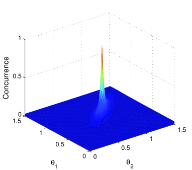
Figure 2: (color online) The concurrence $C$ versus $\theta_{1}$ and $\theta_{2}$. Here we have $\mathcal{Q}=\hat{M}(a_{1},b_{1})U(\theta_{1}),\mathcal{Q^{\prime}}=\hat{M}(a_{2},b_{2})U(\theta_{2})$ with $a_{1}=0.99987,a_{2}=0.01797,U(\theta)=\hat{R}(\theta)\sigma_{z}$ and $\sigma_{z}$ is the Pauli-$z$ matrix. The peak point indicates the maximum concurrence 0.8858 with $\theta_{1}=0.9427$ and $\theta_{2}=0.9428$.

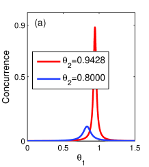
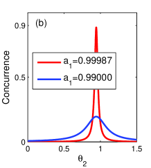
Figure 3: (color online) The concurrence $C$ versus $\theta_{1}$ [in (a)] and $\theta_{2}$ [in (b)]. Here we have $\mathcal{Q}=\hat{M}(a_{1},b_{1})U(\theta_{1}),\mathcal{Q^{\prime}}=\hat{M}(a_{2},b_{2})U(\theta_{2})$ where $U(\theta)=\hat{R}(\theta)\sigma_{z}$. We set $a_{1}=0.99987,a_{2}=0.01797$ [in (a)] and $a_{2}=0.01797,\theta_{1}=0.9427$ [in (b)]. The peak points indicate the maximum concurrence 0.8858 with $\theta_{1}=0.9427$ [in (a)] and $\theta_{2}=0.9428$ [in (b)].

Concluding remark.— In summary, we have presented explicit results on probabilistically improving and maximizing the quantum entanglement of a mixed state through single-qubit operations only. Testing schemes are proposed with numerical simulations. The local operator maximize the outcome entanglement concurrence and can be constructed numerically by iteration. It is interesting to construct the operators directly from the initial $\rho_{\textrm{in}}$ analytically.

References

• (1) L. Amico et al., Rev. Mod. Phys. 80, 517 (2008)
• (2) R. Horodecki et al., Rev. Mod. Phys. 81, 865 (2009)
• (3) M.B. Plenio, V. Vedral, Contemp. Phys. 39, 431 (1998).
• (4) T. Yu, J.H. Eberly, Science 323, 598 (2009).
• (5) O. Jimenez Farias et al., Science, 324, 1414, (2009).
• (6) J. Ma, X. Wang, C. P. Sun, F. Nori, Phys. Reports, in press (2011); arXiv:1011.2978v2
• (7) C.H. Bennett et al., Phys. Rev. Lett. 70, 1895 (1993); M. Zukowski et al., Phys. Rev. Lett. 71, 4287 (1993); J.W. Pan et al., Phys. Rev. Lett. 80, 3891 (1998).
• (8) See e.g., I. Bongioanni et al., arXiv: 1008.5334v1
• (9) M. Tiersch et al., Quantum Inf. Process. 8, 523 (2009).
• (10) W.K. Wootters, Phys. Rev. Lett. 80, 2245 (1998).
• (11) A. Jamiolkowski, Rep. Math. Phys. 3, 275 (1972).
• (12) T. Konrad et al., Nature Physics 4, 99 (2008).