Efficient delay-tolerant particle filtering

Abstract

This paper proposes a novel framework for delay-tolerant particle filtering that is computationally efficient and has limited memory requirements. Within this framework the informativeness of a delayed (out-of-sequence) measurement (OOSM) is estimated using a lightweight procedure and uninformative measurements are immediately discarded. The framework requires the identification of a threshold that separates informative from uninformative; this threshold selection task is formulated as a constrained optimization problem, where the goal is to minimize tracking error whilst controlling the computational requirements. We develop an algorithm that provides an approximate solution for the optimization problem. Simulation experiments provide an example where the proposed framework processes less than 40% of all OOSMs with only a small reduction in tracking accuracy.

I Introduction

Tracking is frequently performed using multiple sensor platforms, with measurements being relayed to a central fusion site over a wireless network. This can lead to some measurements being delayed through packet losses or processing delays. The fusion centre is then faced with out-of-sequence measurements (OOSMs). For some highly non-linear tracking tasks, the particle filter significantly outperforms the Extended or Unscented Kalman Filter (EKFs/UKFs). Incorporating delayed measurements into a particle filter in an efficient manner can be a challenging task. The goal is to retain tracking accuracy while minimizing storage and computational requirements.

In this paper, we propose a novel framework for delay-tolerant particle filtering that is computationally efficient and has limited memory requirements. To derive the framework we formulate a constrained optimization problem of selectively processing only the most informative OOSMs (those that provide the most reduction in tracking error), where the constraint specifies a maximum allowable average computational expenditure. We develop an algorithm that addresses an approximation of this optimization problem. The method combines a Gaussian approximation of the current particle filter distribution and a linearization of the dynamics (similar to the EKF) to derive a procedure for rapidly predicting the anticipated mean squared error reduction associated with processing each OOSM. We then derive a threshold for selecting the “best” OOSMs while respecting the average processing cost constraint. Any measurements which are deemed insufficiently informative are thus immediately discarded.

We report simulation results for an example tracking scenario where the proposed algorithm processes only 40% of all delayed measurements. The algorithm achieves an accuracy that is almost equivalent to that achievable by re-running the particle filter each time a delayed measurement is received, but reduces the computational cost by a factor of almost two.

I-A Related Work

There has been substantial work on the efficient incorporation of out-of-sequence measurements OOSMs in Kalman filters [1, 2, 3, 4, 5, 6, 7, 8, 9]. Fewer techniques have been proposed for processing delayed measurements using particle filters. In [10], Orton et al. propose an approach that stores sets of particles for the last $\ell$ time steps, where $\ell$ is the predetermined maximum delay. The algorithm samples new particles at the time step of the delayed measurement and uses these to update the current particle weights. This method was improved with a Markov chain Monte Carlo (MCMC) smoothing step to mitigate the potential problem of degeneracy in [11]. When a large number of particles is needed for accurate tracking, the algorithm has an excessive storage requirement.

Mallick et al. propose an approximate OOSM particle filter based on retrodiction in [12]. When the filter receives an OOSM, it retrodicts (predicts backwards) the particles to the time step of the delayed measurement and uses these particles to update the current weights. The algorithm in [13] also uses retrodiction, but employs the Gaussian particle filter of [14]. Retrodiction requires a backwards information filter, i.e. a filter that runs backwards in time. Constructing such a filter is possible for linear state dynamics, and these are the systems that are studied in [12, 13]. Recent advances in particle smoothing [15, 16, 17] can be adopted to extend the applicability of these techniques to non-linear systems. However, running the backwards information filter remains a computationally intensive exercise, equivalent to re-running the particle filter from the time of the delayed measurement.

In [15], Orguner et al. develop strategies to reduce both the memory requirements and computational complexity of OOSM particle filters. They propose a “storage efficient particle filter” that only stores statistics (single mean and covariance) of the particle set, rather than the particles themselves, at previous time steps. Auxiliary fixed point smoothers are then employed to determine the likelihood of the delayed measurement conditioned on each particle in the current set, and this likelihood is used to update the weight of each particle. The algorithm can only adjust particle weights, not change particle locations; this can lead to a particle degeneracy problem if an OOSM is highly informative and should induce a significant change in the filtering distribution. Orguner et al. propose a heuristic of ignoring OOSMs that lead to filter degeneracy, but this is not satisfactory, since the highly informative OOSMs are often the most important to process.

The algorithm we propose in this paper involves selective processing of OOSMs. This was first discussed by Orton and Marrs in [10]; they advocated a heuristic approach of discarding all measurements that are delayed beyond a constant time, with the constant to be determined through experiment. More recently, selective OOSM processing has been considered by Tasoulis et al. in [18] and in our previous work [19]. Tasoulis et al. proposed a number of heuristic metrics to estimate the utility of delayed measurements and develop threshold-based tests to discard measurements of low utility. They incorporate these tests into three Kalman filtering algorithms that are designed to process delayed measurements. In [19] we proposed a threshold based procedure to discard uninformative delayed measurements, calculating their informativeness using mutual information and Kullback-Leibler distance metrics. We applied our approach in the general non-linear setting, using a combination of the storage-efficient particle filter proposed in [15] and a re-run particle filter.

The approach proposed by Tasoulis et al. is developed for the Kalman Filter and it is difficult to extend to more general filtering problems with non-linearities. The proposed utility metrics are heuristic and do not truly capture the potential that each delayed measurement has to improve the tracking performance. The latter issue is also a failing of our own work in [19]; although mutual information and Kullback-Leibler distance metrics measure the potential for information gain, they do not directly assess the potential reduction in estimation error. Perhaps most importantly, neither [18] nor [19] identifies a procedure for threshold selection, despite the fact that the choice of this threshold can have a major impact on performance and the appropriate value is a highly application-sensitive quantity.

I-B Paper Organization

The rest of the paper is organized as follows. Section II provides a formal problem statement. Section III describes memory efficient OOSM particle filters. Section IV presents the proposed novel framework for selecting informative OOSMs. In Section V we explore the approximations made in the derivation of the framework and present a theorem identifying asymptotic conditions under which one of the key approximations becomes exact. Section VI presents a concrete OOSM particle filtering algorithm based on the selection framework and Section VII describes simulation experiments for an example tracking scenario. We make concluding remarks in Section VIII.

II Problem Statement

We now provide a formal statement of the OOSM filtering problem that we address and formulate the optimization task. We consider the general discrete-time Markov state-space model with state dynamics and measurement models both defined by non-linear maps. The innovation and observation noises are modelled as additive Gaussian. At each timestep $k$, there is an active set of distributed sensors, $\mathcal{V}_{k}$, that make measurements and $K=\sup_{k\geq 1}|\mathcal{V}_{k}|$ is the maximal number of active sensors. These measurements are relayed to the fusion centre. A subset of them $\mathcal{S}_{k}$ experience minimal delay and can be processed at time $k$. Other measurements are delayed and only become available for processing at later timesteps. Measurements delayed by more than $\ell$ timesteps are discarded.

The system is described by the following state-space model:

$$X_{k} =\mathit{f}_{k}(X_{k-1})+\vartheta_{k}$$ (1)

$$Y_{k}^{s} =\mathit{h}_{k}^{s}(X_{k})+\zeta_{k}^{s}\quad(\forall s\in\mathcal{V}_{k})$$ (2)

$$\mathcal{Y}_{k} =\{Y_{k}^{\mathcal{S}_{k}}:\ \mathcal{S}_{k}\subseteq\mathcal{V}_{k}\}$$ (3)

$$\mathcal{Z}_{k} =\{Y_{k-\ell}^{\mathcal{S}_{k-\ell,k}},Y_{k-\ell+1}^{\mathcal{S}_{k-\ell+1,k}},\ldots,Y_{k-1}^{\mathcal{S}_{k-1,k}}\}$$ (4)

Here $\{X_{k}\}$ denotes the state sequence, which is a Markov diffusion process with initial distribution $X_{0}\sim p(x_{0})$, and $\{Y_{k}^{s}\}$ denotes the measurement sequence at the $s$-th sensor, with $Y_{k}^{\mathcal{S}_{k}}=\{Y_{k}^{s}:s\in\mathcal{S}_{k}\}$. $\vartheta_{k}$ is the innovation noise with Gaussian distribution $\mathcal{N}(0,{\mathbf{V}}_{k})$, and $\zeta_{k}^{s}$ is the measurement noise with Gaussian distribution $\mathcal{N}(0,{\mathbf{Q}}^{s}_{k})$. The functions $\mathit{f}_{k}:\mathbb{R}^{d}\rightarrow\mathbb{R}^{d}$ and $\mathit{h}^{s}_{k}:\mathbb{R}^{d}\rightarrow\mathbb{R}^{m_{s}}$ are the state transition and measurement maps. $\mathcal{Y}_{k}$ denotes the set of non-delayed measurements received at time $k$. $\mathcal{Z}_{k}$ denotes the set of OOSMs received at time $k$. The set $\mathcal{S}_{\tau,k}$ is the subset of active sensors at time $\tau$ whose measurements are received at time step $k$ ($\mathcal{S}_{k,k}\equiv\mathcal{S}_{k}$); $Y_{\tau}^{\mathcal{S}_{\tau,k}}$ is the set of measurements made at time $\tau$ that arrive at the fusion centre at time $k$.

II-1 OOSM Filtering

Let $\mathcal{W}_{i:j,k}$ denote the set of measurements generated in the interval $[i,j]$ available at the fusion centre by time $k$. This includes all the non-delayed measurements $\mathcal{Y}_{i:j}=\bigcup_{m=i}^{j}\mathcal{Y}_{m}$ and OOSMs $\mathcal{Z}_{i:j,k}=\{Z_{\tau,m}^{s}\in\mathcal{Z}_{m}:\tau\in[i,j],s\in\mathcal{S}_{\tau,m},m\in[i+1,k]\}$, where $Z_{\tau,m}^{s}$ is the OOSM that was acquired at time $\tau$ by the sensor $s\in\mathcal{S}_{\tau,m}\subseteq\mathcal{V}_{\tau}$ and was received at the fusion centre at time $m$. Let $\widetilde{\mathcal{W}}_{i:j,k}=\mathcal{W}_{i:j,k}\setminus\mathcal{Z}_{k}=\{\mathcal{W}_{i:j,k-1},\mathcal{Y}_{k}\}$, i.e. the set of all measurements available at time $k$ except those in $\mathcal{Z}_{k}$. Lastly, note that $\mathcal{Z}_{\tau,k}\equiv\mathcal{Z}_{\tau:\tau,k}$, $\mathcal{W}_{\tau,k}\equiv\mathcal{W}_{\tau:\tau,k}$ and $\widetilde{\mathcal{W}}_{\tau,k}\equiv\widetilde{\mathcal{W}}_{\tau:\tau,k}$.

The sequential OOSM filtering task involves calculating an estimate $\widehat{X}_{k}$ of the current state, given all available measurements at time $k$, $\mathcal{W}_{1:k,k}$. In this work, we form the estimate by calculating an approximate expectation of the state by sequentially calculating a particle representation of the posterior distribution.

II-2 Selective Processing for Computational Constraints

In this paper we are interested in reducing computational requirements by processing only the informative OOSMs. We formulate this problem as an optimization problem that involves minimizing the mean-squared error (with respect to an $L_{2}$ norm) subject to satisfying a constraint ($C_{ave}$) on the expected computation at each time step.

Let $b_{\tau,k}^{s}\in\{0,1\}$ be the indicator of OOSM $Z_{\tau,k}^{s}$ arrival and denote by $p_{\tau,k}^{s}$ the expected value of $b_{\tau,k}^{s}$, conditioned on all the measurements received prior to time $k$. Denote by $C_{\tau,k}^{s}$ the computational cost associated with processing the OOSM $Z_{\tau,k}^{s}$. Let $d_{\tau,k}^{s}\in\{0,1\}$ be our decision to process or reject measurement $Z_{\tau,k}^{s}$ and $\mathcal{D}_{k}=\bigcup_{\tau=k-\ell}^{k-1}\bigcup_{s\in\mathcal{S}_{\tau,k}}\{d_{\tau,k}^{s}\}$ be the current set of all possible decisions. Decisions must be made sequentially, prior to the arrivals of the OOSMs at time $k$ due to the real-time nature of the tracking task. The goal is to ensure that the computational constraint is obeyed on average at each time step, i.e. in expectation with respect to all possible arrivals of OOSMs.

We thus address the following optimization task for each $k$ over the tracking period:

$$\min_{\mathcal{D}_{k}\in\{0,1\}^{\sum_{\tau}|\mathcal{V}_{\tau}|}}{\mathbb{E}}\left\{|X_{k}-\widehat{X}_{k}|^{2}\right\}$$

$$\text{subject to}\quad\sum_{k=1}^{K}\sum_{\tau=k-\ell}^{k-1}\sum_{s\in\mathcal{D}_{\tau,k}}d_{\tau,k}^{s}p_{\tau,k}^{s}C_{\tau,k}^{s}\leq KC_{\mathrm{ave}}$$ (5)

III OOSM Particle Filters

Previously proposed OOSM particle filters primarily differ in how they incorporate the OOSMs from the set $\mathcal{Z}_{k}$. The simplest approach is to discard them, but this often results in poor tracking performance. Another obvious approach is to restart the filter at the time step immediately prior to the time step associated with the earliest OOSM in $\mathcal{Z}_{k}$ and re-run to the current time step $k$. This requires that we record all the particles, weights and the measurements for the maximal delay window. We call this approach the “OOSM re-run particle filter” and consider it to be an accuracy benchmark. This method has two unattractive qualities: the storage requirements can be immense and the computation cost is high.

As discussed in Section I-A, several methods have been proposed to alleviate these costs. In this section, we provide a brief review of the storage efficient particle filter of [15] and describe a relatively obvious alternative algorithm that we introduced in [19]. In both algorithms, the memory requirements are reduced by storing statistics of the particle sets from past time steps instead of the particles themselves. The past particle distributions are approximated by Gaussian approximations. The stored information is then the mean and covariance matrix of particles at each time step from $k-\ell-1$ to $k$. Denote, respectively, by ${\bm{\xi}}_{k}$, ${\bm{\omega}}_{k}$ the sets of the values and weights of particles at time $k$, and let ${\bm{\mu}}_{k}$, ${\mathbf{R}}_{k}$ denote their mean and covariance. The stored information is then

$${\mathbf{\Omega}}_{k} =\{{\bm{\mu}}_{k-\ell:k},{\mathbf{R}}_{k-\ell:k},\mathcal{W}_{k-\ell-1:k,k}\},$$ (6)

Here ${\bm{\mu}}_{k-\ell-1:k}$ and ${\mathbf{R}}_{k-\ell-1:k}$ denote, respectively, the means and covariances of the particle sets for time-steps ranging from $k-\ell-1$ to $k$.

A generic storage efficient OOSM particle filtering algorithm is summarized in Algorithm 1. If there are no OOSMs at time $k$, we write $\mathcal{Z}_{k}=\emptyset$.

At time $k$

Input: $\mathcal{Z}_{k}$, ${\mathbf{\Omega}}_{k-1}$, ${\bm{\xi}}_{k-1}$, ${\bm{\omega}}_{k-1}$,$\mathcal{Y}_{k}$

(${\bm{\xi}}_{k}$, ${\bm{\omega}}_{k}$) $\leftarrow$ ParticleFilter($\mathcal{Y}_{k}$, ${\bm{\xi}}_{k-1}$, ${\bm{\omega}}_{k-1}$) ;

(${\bm{\mu}}_{k}$, ${\mathbf{R}}_{k}$) $\leftarrow$ SaveGauss(${\bm{\xi}}_{k}$, ${\bm{\omega}}_{k}$) ;

if $\mathcal{Z}_{k}\neq\emptyset$ then

(${\bm{\xi}}_{k}$, ${\bm{\omega}}_{k}$, ${\mathbf{\Omega}}_{k}$) $\leftarrow$ ProcessOOSM($\mathcal{Z}_{k}$, ${\bm{\xi}}_{k}$, ${\bm{\omega}}_{k}$, ${\mathbf{\Omega}}_{k}$);

Algorithm 1 Generic OOSM Particle Filter

In this algorithm, the function ParticleFilter can be any standard particle filtering method. If $\mathcal{Y}_{k}=\emptyset$, ParticleFilter only propagates the particles and skips the measurement processing step. The function SaveGauss calculates the maximum likelihood estimates of the mean and covariance given the weighted sample set ${\bm{\xi}}_{k}$, ${\bm{\omega}}_{k}$ and stores these in ${\mathbf{\Omega}}_{k}$:

$${\bm{\mu}}_{k} =\sum_{i=1}^{N}{\bm{\omega}}_{k}^{(i)}{\bm{\xi}}_{k}^{(i)}$$ (7)

$${\mathbf{R}}_{k} =\sum_{i=1}^{N}{\bm{\omega}}_{k}^{(i)}({\bm{\xi}}_{k}^{(i)}-{\bm{\mu}}_{k})({\bm{\xi}}_{k}^{(i)}-{\bm{\mu}}_{k})^{T}$$ (8)

The function ProcessOOSM specifies how OOSMs are processed and varies depending on the specific algorithm.

11

11

11

11

11

11

11

11

11

11

11

III-A Gaussian Approximation Re-run Particle Filter (OOSM-GARP)

A simple modification of the re-run particle filter involves storing only Gaussian approximations of the particle distributions at previous timesteps. When a batch of OOSMs arrives, the particle filter is re-run from the time step preceding the earliest OOSM. Since the particle set from that time step is unavailable, particles are generated from the stored approximation.

When OOSM-GARP receives $\mathcal{Z}_{k}$ at time $k$, it returns to the time step $\widetilde{\tau}_{k}-1$ (let $\widetilde{\tau}_{k}$ denote the earliest time step of all OOSMs in $\mathcal{Z}_{k}$). It samples particles from $\mathcal{N}({\bm{\mu}}_{\widetilde{\tau}_{k}-1},{\mathbf{R}}_{\widetilde{\tau}_{k}-1})$, propagates them to the time step $\widetilde{\tau}_{k}$ and runs the filter as standard particle filter using all stored measurements. At each step, it updates the mean and covariance matrix in the stored set ${\mathbf{\Omega}}_{k}$ as described in Algorithm 2.

Input: $\mathcal{Z}_{k}$, ${\mathbf{\Omega}}_{k}$

$\widetilde{\tau}_{k}=\min\limits_{\tau}\{\tau:y_{\tau}\in\mathcal{Z}_{k}\}$ ;

$\{{\bm{\xi}}_{\widetilde{\tau}_{k}-1}^{(i)}\}_{i=1}^{N}$ $\sim$ $\mathcal{N}(x_{\widetilde{\tau}_{k}-1},{\bm{\mu}}_{\widetilde{\tau}_{k}-1},{\mathbf{R}}_{\widetilde{\tau}_{k}-1})$ ;

${\bm{\omega}}_{\widetilde{\tau}_{k}-1}^{(i)}=1/N,\ i=1\ldots N$ ;

for $j=\widetilde{\tau}_{k},\ldots,k$ do

(${\bm{\xi}}_{j}$, ${\bm{\omega}}_{j}$) $\leftarrow$ ParticleFilter($\mathcal{W}_{j,k}$, ${\bm{\xi}}_{j-1}$, ${\bm{\omega}}_{j-1}$);

(${\bm{\mu}}_{j}$, ${\mathbf{R}}_{j}$) $\leftarrow$ SaveGauss(${\bm{\xi}}_{j}$, ${\bm{\omega}}_{j}$) ;

endfor

Algorithm 2 ProcessOOSM-GARP

13

13

13

13

13

13

13

13

13

13

13

13

13

In many tracking tasks, the Gaussian provides a reasonable approximation to the particle distributions. In OOSM-GARP, the Gaussian is only used to re-start the particle filter (to draw initial samples), so the impact of approximation errors on filtering performance is relatively small. OOSM-GARP thus performs almost as well as the basic re-run particle filter but requires much less memory. However, OOSM-GARP is relatively computationally complex since it reprocesses all the particles for $k-\widetilde{\tau}_{k}+1$ steps. Note that the cost to process OOSMs corresponding to a single time step, $\mathcal{Z}_{j,k}$, is approximately equal to that of processing the whole batch of OOSMs $\mathcal{Z}_{j:k-1,k}$ since we have to execute the particle filter from time $j$ to time $k$ in both cases. This cost is proportional to the total computational complexity of functions ParticleFilter and SaveGauss multiplied by a factor of $k-j$.

III-B Storage Efficient Particle Filter with EKS (SEPF-EKS)

We now provide a brief review of the storage efficient OOSM particle filter from [15]. Orguner et al. described three versions of the filter, which differed according to the auxiliary fixed-point smoother they employed. We focus on the filter that employs Extended Kalman Smoother, since it is the least computationally demanding but has comparable tracking performance.

The SEPF is based on the following weight-update equation:

$${\bm{\omega}}_{k}^{(i)} \propto p(\mathcal{Z}_{\tau,k}|{\bm{\xi}}_{k}^{(i)},\widetilde{\mathcal{W}}_{{1:k},k}){\bm{\omega}}_{k,\bar{\tau}}^{(i)}.$$ (9)

Here ${\bm{\omega}}_{k,\bar{\tau}}^{(i)}$ and ${\bm{\omega}}_{k}^{(i)}$ denote the weights before and after processing $\mathcal{Z}_{\tau,k}$. The SEPF estimates this likelihood expression in two stages. First it approximates $p(x_{\tau}|{\bm{\xi}}_{k}^{(i)},\widetilde{\mathcal{W}}_{{1:k},k})$ by applying an augmented-state extended Kalman smoother [20], treating the current particle ${\bm{\xi}}_{k}^{(i)}$ as a measurement. The SEPF then employs an EKF approximation of $p(\mathcal{Z}_{\tau,k}|x_{\tau})$ to construct an estimate of the likelihood $p(\mathcal{Z}_{\tau,k}|{\bm{\xi}}_{k}^{(i)},\widetilde{\mathcal{W}}_{{1:k},k})$.

Although the original algorithm was designed to treat individual OOSMs, it can be easily extended to treat batches of OOSMs by running a separate update for each time-step. This extended algorithm is presented as Algorithm 3.

Input: $\mathcal{Z}_{k}$, ${\mathbf{\Omega}}_{k}$, ${\bm{\omega}}_{k,\bar{\tau}}$, ${\bm{\xi}}_{k}$

for $\mathcal{Z}_{\tau,k}\in\mathcal{Z}_{k}$ do

Compute approximation $p(\mathcal{Z}_{\tau,k}|{\bm{\xi}}_{k}^{(i)},\widetilde{\mathcal{W}}_{{1:k},k})$ for all $i$;

${\bm{\omega}}_{k}^{(i)}$ $\leftarrow$ ${\bm{\omega}}_{k,\bar{\tau}}^{(i)}p(\mathcal{Z}_{\tau,k}|{\bm{\xi}}_{k}^{(i)},\widetilde{\mathcal{W}}_{{1:k},k})$ $\forall i$ ;

endfor

${\bm{\omega}}_{k}={\bm{\omega}}_{k}/\sum_{i}{\bm{\omega}}_{k}^{(i)}$ ;

Algorithm 3 ProcessSEPF-EKS

11

11

11

11

11

11

11

11

11

11

11

SEPF-EKS achieves significant computational savings because the filtering operations for step $2$ are common to all $N$ particles except for a single time-step. This means that the effective computational cost is equivalent to running one time step of a particle filter, and is therefore usually less than that of the OOSM-GARP filter. The advantage diminishes when it is common for OOSMs to arrive in batches with different delays because of the seemingly unavoidable loop in the algorithm.

IV Selective OOSM Processing

The computational cost of processing an OOSM is relatively high and frequently it is wasted effort, resulting in minimal change to the filtering distribution or the tracking accuracy. In this section we design a procedure for addressing the optimization problem posed in Section II, that of minimizing the mean squared error while controlling the computational effort.

The optimization problem is challenging and generating an exact solution would be more costly than simply processing all OOSMs with a re-run particle filter. We therefore strive to approximate the problem so that we can develop an efficient procedure for selecting the informative OOSMs. The complexity of this procedure must not depend on the number of particles in the filter.

Our method employs a Gaussian approximation of the joint distribution of the current state and the current set of OOSMs. We derive this approximation using an EKF-type linear approximation of the general state-space model. Second, we model the OOSMs from different sensors or different times as approximately unconditionally independent. This second approximation allows us to disentangle the effects of processing different OOSMs on the filtering error. In section V we study asymptotic conditions under which this assumption holds exactly. This provides a solid theoretical justification for our choice of this simplifying approximation and we consider that it is sufficiently accurate in practice for our purpose of selecting the informative OOSMs. It is important to stress that these approximations are only used for the purpose of selecting the measurements to process; they are not employed within the filter itself.

IV-A Tracking MSE Under Gaussian Approximation

We employ the well known EKF-type linear approximation of the general state-space model:

$$X_{k} =f_{k}(\mu_{X_{k-1}})+{\mathbf{F}}_{k}(X_{k-1}-\mu_{X_{k-1}})+\vartheta_{k}$$ (10)

$$Y_{k}^{s} =h_{k}^{s}(\mu_{X_{k}})+{\mathbf{H}}_{k}^{s}(X_{k}-\mu_{X_{k}})+\zeta_{k}^{s},\quad\quad\quad s\in\mathcal{V}_{k}$$ (11)

Here ${\mathbf{F}}_{k}$ and ${\mathbf{H}}_{k}^{s}$ are linearizations (through Taylor expansion at $\mu_{X_{k-1}}$ and $\mu_{X_{k}}$, respectively) of the non-linear dynamic and measurement maps.

Let ${\mathbf{P}}_{k}$ and $\mu_{k}$ be the covariance matrix and the mean of the Gaussian approximation of the joint probability distribution of the current state and the current set of OOSMs conditioned on all available measurements. The covariance matrix and the mean have the following structure:

$${\mathbf{P}}_{k}=\begin{pmatrix}{\mathbf{R}}_{X_{k}X_{k}|\widetilde{\mathcal{W}}_{1:k,k}}&{\mathbf{R}}_{X_{k}\mathcal{Z}_{k}|\widetilde{\mathcal{W}}_{1:k,k}}\\ {\mathbf{R}}_{\mathcal{Z}_{k}X_{k}|\widetilde{\mathcal{W}}_{1:k,k}}&{\mathbf{R}}_{\mathcal{Z}_{k}\mathcal{Z}_{k}|\widetilde{\mathcal{W}}_{1:k,k}}\end{pmatrix},\,\mu_{k}=\begin{pmatrix}\mu_{X_{k}|\widetilde{\mathcal{W}}_{1:k,k}}\\ \mu_{\mathcal{Z}_{k}|\widetilde{\mathcal{W}}_{1:k,k}}\end{pmatrix}$$ (12)

where ${\mathbf{R}}_{X_{k}X_{k}|\widetilde{\mathcal{W}}_{1:k,k}}$ is the current state covariance, ${\mathbf{R}}_{X_{k}\mathcal{Z}_{k}|\widetilde{\mathcal{W}}_{1:k,k}}$ and ${\mathbf{R}}_{\mathcal{Z}_{k}X_{k}|\widetilde{\mathcal{W}}_{1:k,k}}={\mathbf{R}}_{X_{k}\mathcal{Z}_{k}|\widetilde{\mathcal{W}}_{1:k,k}}^{T}$ is the state-measurement cross-covariance and ${\mathbf{R}}_{\mathcal{Z}_{k}\mathcal{Z}_{k}|\widetilde{\mathcal{W}}_{1:k,k}}$ is the measurement set covariance. Note that the means and covariances are conditioned on $\widetilde{\mathcal{W}}_{1:k,k}$ which includes the current set of undelayed measurements $\mathcal{Y}_{k}$ as well as all the OOSMs and undelayed measurements that have been incorporated up to time $k$. In the following discussion, we will often skip this conditioning to avoid unnecessarily complicated notation, but this conditioning is implied unless explicitly stated otherwise.

The optimal MMSE estimator $\widehat{X}_{k}$ of the state is known to be the conditional mean $\mu_{X_{k}|\widetilde{\mathcal{W}}_{1:k,k},\mathcal{Z}_{k}}$, which in the case of our Gaussian approximation is simply:

$$\widehat{X}_{k}=\mu_{X_{k}}+{\mathbf{R}}_{X_{k}\mathcal{Z}_{k}}{\mathbf{R}}_{\mathcal{Z}_{k}\mathcal{Z}_{k}}^{-1}(\mathcal{Z}_{k}-\mu_{\mathcal{Z}_{k}}).$$ (13)

Let $\mathcal{B}_{k}=\bigcup_{\tau=k-\ell}^{k-1}\bigcup_{s\in\mathcal{S}_{\tau,k}}\{b_{\tau,k}^{s}\}$ be the set of random variables that indicate OOSM arrivals at time $k$. This set defines the structure of the set $\mathcal{Z}_{k}$ along with the associated mean $\mu_{\mathcal{Z}_{k}}$ and (cross-)covariance terms ${\mathbf{R}}_{X_{k}\mathcal{Z}_{k}}$ and ${\mathbf{R}}_{\mathcal{Z}_{k}\mathcal{Z}_{k}}$. By the law of total variance the variance of the the estimator can be expressed as:

$$\mathrm{var}(X_{k}-\widehat{X}_{k})= {\mathbb{E}}\{\mathrm{var}(X_{k}-\widehat{X}_{k}|\mathcal{B}_{k})\}+\mathrm{var}({\mathbb{E}}\{X_{k}-\widehat{X}_{k}|\mathcal{B}_{k}\}).$$ (14)

Since, according to our linearization, ${\mathbb{E}}\{X_{k}|\mathcal{B}_{k}\}=f_{k}(\mu_{X_{k-1}})$ and ${\mathbb{E}}\{\widehat{X}_{k}|\mathcal{B}_{k}\}=\mu_{X_{k}}=f_{k}(\mu_{X_{k-1}})$ we have for any realization of $\mathcal{B}_{k}$: ${\mathbb{E}}\{X_{k}-\widehat{X}_{k}|\mathcal{B}_{k}\}=0$. Thus the variance of the MMSE estimator is equal to the expectation of its variance conditioned on the realization of indicators $\mathcal{B}_{k}$:

$$\mathrm{var}(X_{k}-\widehat{X}_{k})={\mathbb{E}}\{\mathrm{var}(X_{k}-\widehat{X}_{k}|\mathcal{B}_{k})\}.$$ (15)

For a specific realization of indicators $\mathcal{B}_{k}$ this variance is defined by the components of the joint covariance matrix (recall that $\mathcal{Z}_{k}$ is a function of $\mathcal{B}_{k}$):

$$\mathrm{var}(X_{k}-\widehat{X}_{k}|\mathcal{B}_{k})={\mathbf{R}}_{X_{k}X_{k}}-{\mathbf{R}}_{X_{k}\mathcal{Z}_{k}}{\mathbf{R}}_{\mathcal{Z}_{k}\mathcal{Z}_{k}}^{-1}{\mathbf{R}}_{\mathcal{Z}_{k}X_{k}}$$ (16)

The mean squared error of estimating the state $X_{k}$ conditioned on the OOSM set $\mathcal{Z}_{k}$ (as well as all the previous measurements) is thus given by

$$\operatorname{tr}\mathrm{var}(X_{k}-\widehat{X}_{k}) ={\mathbb{E}}\{\operatorname{tr}\mathrm{var}(X_{k}-\widehat{X}_{k}|\mathcal{B}_{k})\}$$ (17)

$$=\operatorname{tr}{\mathbf{R}}_{X_{k}X_{k}}-{\mathbb{E}}\{\operatorname{tr}{\mathbf{R}}_{X_{k}\mathcal{Z}_{k}}{\mathbf{R}}_{\mathcal{Z}_{k}\mathcal{Z}_{k}}^{-1}{\mathbf{R}}_{\mathcal{Z}_{k}X_{k}}\}$$ (18)

Under the assumption that the measurements made by different sensors (or the same sensor at different times) are approximately unconditionally independent, ${\mathbf{R}}_{\mathcal{Z}_{k}\mathcal{Z}_{k}}$ is approximately block-diagonal. This implies that we can approximate the above expression as follows:

$$\operatorname{tr}\mathrm{var}(X_{k}-\widehat{X}_{k})\approx\operatorname{tr}{\mathbf{R}}_{X_{k}X_{k}}-{\mathbb{E}}\left\{\sum_{\tau=k-\ell}^{k-1}\sum_{s\in\mathcal{V}_{\tau}}d_{\tau,k}^{s}b_{\tau,k}^{s}\operatorname{tr}{\mathbf{R}}_{X_{k}Y_{\tau}^{s}}{\mathbf{R}}_{Y_{\tau}^{s}Y_{\tau}^{s}}^{-1}{\mathbf{R}}_{Y_{\tau}^{s}X_{k}}\right\}.$$ (19)

Here the expectation is taken with respect to the measurement arrival indicators $b_{\tau,k}^{s}$, ${\mathbf{R}}_{Y_{\tau}^{s}Y_{\tau}^{s}}=\mathrm{var}(Y_{\tau}^{s})$ is measurement covariance and ${\mathbf{R}}_{Y_{\tau}^{s}X_{k}}=\mathrm{cov}(Y_{\tau}^{s},X_{k})$ is the state-measurement cross covariance. If we denote

$$R_{\tau,k}^{s}=\operatorname{tr}{\mathbf{R}}_{X_{k}Y_{\tau}^{s}}{\mathbf{R}}_{Y_{\tau}^{s}Y_{\tau}^{s}}^{-1}{\mathbf{R}}_{Y_{\tau}^{s}X_{k}},$$ (20)

the factor that we will refer to as the measurement utility then the expression for the MSE can be further simplified:

$$\operatorname{tr}\mathrm{var}(X_{k}-\widehat{X}_{k})\approx\operatorname{tr}{\mathbf{R}}_{X_{k}X_{k}}-\sum_{\tau=k-\ell}^{k-1}\sum_{s\in\mathcal{V}_{\tau}}d_{\tau,k}^{s}p_{\tau,k}^{s}R_{\tau,k}^{s}.$$ (21)

where $p_{\tau,k}^{s}={\mathbb{E}}\left\{b_{\tau,k}^{s}\right\}$ is the probability that the measurement acquired by sensor $s$ at time $\tau$ arrives at time $k$ (conditioned on the measurement arrivals up to time $k$). The above expression is a natural objective function to be minimized to assure the best tracking quality. The minimal value of the objective is reached when all measurements are processed ($d_{\tau,k}^{s}=1,\forall\,\tau,s$) since $R_{\tau,k}^{s}\geq 0$.

IV-B One-step Constrained Minimization of Approximate MSE

Given the discussion above and the identified approximations, the constrained optimization problem posed in Section II can be formulated as follows:

$$\min_{\mathcal{D}_{k}\in\{0,1\}^{\sum_{\tau}|\mathcal{V}_{\tau}|}}\operatorname{tr}\mathrm{var}(X_{k}-\widehat{X}_{k})$$

$$\quad\text{subject to}\quad\sum_{\tau=k-\ell}^{k-1}\sum_{s\in\mathcal{D}_{\tau,k}}d_{\tau,k}^{s}p_{\tau,k}^{s}C_{\tau,k}^{s}\leq C_{\mathrm{ave}}$$ (22)

The unconstrained objective to be minimized can be formulated using Lagrange relaxation with Lagrange multiplier $\gamma_{k}$:

$$J(\mathcal{D}_{k}) =\operatorname{tr}\mathrm{var}(X_{k}-\widehat{X}_{k})+\gamma_{k}\left(\sum_{\tau=k-\ell}^{k-1}\sum_{s\in\mathcal{V}_{\tau}}d_{\tau,k}^{s}p_{\tau,k}^{s}C_{\tau,k}^{s}-C_{\mathrm{ave}}\right)$$

$$=\operatorname{tr}{\mathbf{R}}_{X_{k}X_{k}}-\sum_{\tau=k-\ell}^{k-1}\sum_{s\in\mathcal{V}_{\tau}}d_{\tau,k}^{s}p_{\tau,k}^{s}(R_{\tau,k}^{s}-\gamma_{k}C_{\tau,k}^{s})-\gamma_{k}C_{\mathrm{ave}}.$$ (23)

For a fixed $\gamma_{k}$ the optimal solution can be found by optimizing each $d_{\tau,k}^{s}$ independently since the contribution of each term under the sum corresponding to a particular $d_{\tau,k}^{s}$ is independent of all other variables to be optimized. It is clear that setting $d_{\tau,k}^{s}=1$ whenever $R_{\tau,k}^{s}-\gamma_{k}C_{\tau,k}^{s}\geq 0$ and $d_{\tau,k}^{s}=0$ whenever $R_{\tau,k}^{s}-\gamma_{k}C_{\tau,k}^{s}<0$ produces the smallest value of the objective function for a given $\gamma_{k}$. Substituting this solution into the constraint we obtain

$$\sum_{\tau=k-\ell}^{k-1}\sum_{s\in\mathcal{V}_{\tau}}{\textbf{1}}_{\{R_{\tau,k}^{s}-\gamma_{k}C_{\tau,k}^{s}\}}p_{\tau,k}^{s}C_{\tau,k}^{s}\leq C_{\mathrm{ave}},$$ (24)

where ${\textbf{1}}_{\{\cdot\}}$ is the indicator function. If we denote $\widetilde{R}_{\tau,k}^{s}=R_{\tau,k}^{s}/C_{\tau,k}^{s}$, the measurement utility diminished by the processing cost incurred, the above is equivalent to

$$\sum_{\{s,\tau:\widetilde{R}_{\tau,k}^{s}\geq\gamma_{k}\}}p_{\tau,k}^{s}C_{\tau,k}^{s}\leq C_{\mathrm{ave}}.$$ (25)

The optimal value of $\gamma_{k}$ is thus the smallest value for which (25) holds. A simple practical algorithm can be devised to identify this value of $\gamma_{k}$. The algorithm, summarized in Algorithm 4, assumes that we can evaluate $p_{\tau,k}^{s}$, which is usually possible given sufficient knowledge about the measurement apparatus and the network delay profile.

Input: $\{\widetilde{R}_{\tau,k}^{s}\}$, $\{p_{\tau,k}^{s}\}$, $\{C_{\tau,k}^{s}\}$ of cardinality $T=\sum_{\tau=k-\ell}^{k-1}|\mathcal{V}_{\tau}|$ and $C_{\mathrm{ave}}$ ;

Order set $\{\widetilde{R}_{\tau,k}^{s}\}$ by decreasing value, output ordered sequence $\{R_{n}^{o}\}_{n=1}^{T}$ ;

Construct sequences $\{p_{n}^{o}\}_{n=1}^{T}$, $\{C_{n}^{o}\}_{n=1}^{T}$ using mapping $(\tau,s)\mapsto n$ used for the previous set ;

Construct sequence $\{\Psi_{n}^{o}\}_{n=1}^{T}$ with elements $\Psi_{n}^{o}=\sum_{j=1}^{n}p_{j}^{o}C_{j}^{o}$

Identify $n^{*}=\arg\max_{n}\Psi_{n}^{o}:\Psi_{n}^{o}\leq C_{ave}$

Output: $\gamma_{k}=R_{n^{*}}^{o}$ ;

Algorithm 4 Threshold selection algorithm

9

9

9

9

9

9

9

9

9

We can now describe the operation of the proposed OOSM selection algorithm. At every filtering step the selection algorithm first calculates the measurement utilities diminished by the processing cost, $\widetilde{R}_{\tau,k}^{s}$, along with probabilities of arrival for all possible OOSMs, $p_{\tau,k}^{s}$. It then identifies a threshold $\gamma_{k}$ such that the expected processing cost does not exceed $C_{ave}$ (step 4 in Algorithm 4). The final step of the algorithm is to select arriving OOSMs with utility $\widetilde{R}_{\tau,k}^{s}$ surpassing the calculated threshold.

To execute the proposed algorithm we need expressions for the (cross-) covariance matrices ${\mathbf{R}}_{X_{k}Y_{\tau}^{s}}$ and ${\mathbf{R}}_{Y_{\tau}^{s}Y_{\tau}^{s}}$. These matrices can be calculated online using the extended Kalman smoother (EKS) algorithm. We employ the Rauch-Tung-Striebel (RTS) backward recursion realization [21]. We apply the RTS recursion starting from the Gaussian approximation of the posterior at the current time $k$ and moving backwards in time until time step $k-\ell$. As a result, we obtain a sequence of smoother means $\mu_{X_{\tau}|\widetilde{\mathcal{W}}_{1:k,k}}$ and covariance matrices ${\mathbf{R}}_{X_{\tau}X_{\tau}}$ for $k-\ell\leq\tau<k$.

At time $k$ we have the set of measurements $\widetilde{\mathcal{W}}_{1:k,k}$, so the linearizations (10) can be made more general (and, hopefully, accurate) with the use of the EKS statistics $\mu_{X_{\tau}|\widetilde{\mathcal{W}}_{1:k,k}},\tau<k-1$:

$$X_{\tau} =f_{\tau}(\mu_{X_{\tau-1}|\widetilde{\mathcal{W}}_{1:k,k}})+{\mathbf{F}}_{\tau}(X_{\tau-1}-\mu_{X_{\tau-1}|\widetilde{\mathcal{W}}_{1:k,k}})+\vartheta_{\tau}$$ (26)

$$Y_{\tau}^{s} =h_{\tau}^{s}(\mu_{X_{\tau}|\widetilde{\mathcal{W}}_{1:k,k}})+{\mathbf{H}}_{\tau}^{s}(X_{\tau}-\mu_{X_{\tau}|\widetilde{\mathcal{W}}_{1:k,k}})+\zeta_{\tau}^{s},\ s\in\mathcal{V}_{\tau}.$$ (27)

Here the Jacobians ${\mathbf{F}}_{\tau}$ and ${\mathbf{H}}_{\tau}^{s}$ are evaluated at the points defined by the respective EKS means. With the use of the above linearization, calculation of the required approximate covariance matrices becomes straightforward. Noting that ${\mathbb{E}}\{Y_{\tau}^{s}\}=h_{\tau}^{s}(\mu_{X_{\tau}})$, and observing the independence of $\zeta_{\tau}^{s}$ and $X_{\tau}-\mu_{X_{\tau}}$, we can derive

$${\mathbf{R}}_{Y_{\tau}^{s}Y_{\tau}^{s}}={\mathbf{H}}_{\tau}^{s}{\mathbf{R}}_{X_{\tau}X_{\tau}}{{\mathbf{H}}_{\tau}^{s}}^{T}+{\mathbf{R}}_{\zeta_{\tau}^{s}\zeta_{\tau}^{s}}.$$ (28)

Note that ${\mathbf{R}}_{X_{\tau}X_{\tau}}$ is the covariance of the extended Kalman smoother.

Next, we calculate the cross-covariance ${\mathbf{R}}_{X_{k}Y_{\tau}^{s}}$. Since ${\mathbb{E}}\{X_{\tau}\}=f_{\tau}(\mu_{X_{\tau-1}})$, we have for any $\tau<k$:

$$X_{k}-{\mathbb{E}}\{X_{k}\} ={\mathbf{F}}_{k}(X_{k-1}-\mu_{X_{k-1}})+\vartheta_{k}$$ (29)

$$={\mathbf{F}}_{k}({\mathbf{F}}_{k-1}(X_{k-2}-\mu_{X_{k-2}})+\vartheta_{k-1})+\vartheta_{k}$$ (30)

$$={\mathbf{F}}_{k}{\mathbf{F}}_{k-1}({\mathbf{F}}_{k-2}(X_{k-3}-\mu_{X_{k-3}})+\vartheta_{k-2})+{\mathbf{F}}_{k}\vartheta_{k-1}+\vartheta_{k}$$ (31)

$$={\mathbf{F}}_{k,\tau}(X_{\tau}-\mu_{X_{\tau}})+\sum_{j=\tau+1}^{k}{\mathbf{F}}_{k,j}\vartheta_{j}$$ (32)

where we have introduced the notation ${\mathbf{F}}_{k,\tau}=\prod_{j=\tau+1}^{k}{\mathbf{F}}_{j}$ and ${\mathbf{F}}_{k,k}={\mathbf{I}}$. We can thus evaluate the cross-covariance using the expression:

$${\mathbf{R}}_{X_{k}Y_{\tau}^{s}}={\mathbf{F}}_{k,\tau}{\mathbf{R}}_{X_{\tau}X_{\tau}}{{\mathbf{H}}_{\tau}^{s}}^{T}.$$ (33)

V Asymptotic Optimality of the Proposed Algorithm

In this section we will consider the conditions under which the unconditional measurement independence approximation made in the previous section is expected to hold, assuming that the Gaussian approximation is accurate. The assumption simplifies the algorithm derivation and reduces its computational requirements, but it leads to sub-optimality of the derived constrained MSE minimization algorithm. The conditions established in this section help us understand when the performance of the proposed sub-optimal algorithm is expected to approach that of the optimal OOSM selection algorithm, assuming that the Gaussian approximation and linearization are accurate.

The following theorem specifies that, under mild regularity assumptions, if an asymptotic condition on the minimal eigenvalues of the noise matrices holds, then the block-diagonal approximation employed to derive the OOSM selection algorithm in the previous section holds exactly. The proof is provided in Appendix A.

Theorem 1.

Let ${\mathbf{R}}_{\mathcal{Z}_{k}\mathcal{Z}_{k}}$, ${\mathbf{R}}_{X_{k}\mathcal{Z}_{k}}$ be defined as in (12) and let ${\mathbf{B}}_{\mathcal{Z}_{k}\mathcal{Z}_{k}}$ be the block-diagonal matrix whose diagonal blocks match those of ${\mathbf{R}}_{\mathcal{Z}_{k}\mathcal{Z}_{k}}$ (the covariances of measurements from the same sensor at the same time). Suppose that the following assumptions hold:

• $\rho({\mathbf{R}}_{X_{n}X_{n}})<\infty$, $\forall k-\ell\leq n<k$

• $\rho({\mathbf{H}}_{m}^{s}{{\mathbf{H}}_{m}^{s}}^{T})^{1/2}<\infty$ and $\rho({{\mathbf{H}}_{m}^{s}}^{T}{\mathbf{H}}_{m}^{s})^{1/2}<\infty$, $\forall k-\ell\leq m<k$ and $\forall s\in\mathcal{V}_{m}$

• $\rho({\mathbf{F}}_{m,n}{\mathbf{F}}_{m,n}^{T})^{1/2}<\infty$, $\forall k-\ell\leq n\leq m$ and $k-\ell\leq m\leq k$

Then we have for any $\ell,K<\infty$, $\mathcal{Z}_{k}$ and $k>1$:

$$\min_{s,m}\lambda_{\min}({\mathbf{R}}_{\zeta_{m}^{s}\zeta_{m}^{s}})\rightarrow\infty\Rightarrow|\operatorname{tr}{\mathbf{R}}_{X_{k}\mathcal{Z}_{k}}{\mathbf{R}}_{\mathcal{Z}_{k}\mathcal{Z}_{k}}^{-1}{\mathbf{R}}_{\mathcal{Z}_{k}X_{k}}-\operatorname{tr}{\mathbf{R}}_{X_{k}\mathcal{Z}_{k}}{\mathbf{B}}_{\mathcal{Z}_{k}\mathcal{Z}_{k}}^{-1}{\mathbf{R}}_{\mathcal{Z}_{k}X_{k}}|\rightarrow 0,$$ (34)

where $\lambda_{\min}(\cdot)=\min_{i}\lambda_{i}(\cdot)$

The regularity conditions imposed in Theorem 1 are mild and natural. Assumption $\mathcal{A}_{1}$ requires the extended Kalman smoother covariance ${\mathbf{R}}_{X_{n}X_{n}}$ to have finite spectral radius. Thus assumption $\mathcal{A}_{1}$ basically requests the stability (including the numerical stability) of the EKS. Assumption $\mathcal{A}_{2}$ and $\mathcal{A}_{3}$ require the spectral radia of matrices ${\mathbf{H}}_{m}^{s}{{\mathbf{H}}_{m}^{s}}^{T}$, ${{\mathbf{H}}_{m}^{s}}^{T}{\mathbf{H}}_{m}^{s}$ and ${\mathbf{F}}_{m,n}{\mathbf{F}}_{m,n}^{T}$ to be finite. If the measurement and transition functions, $h_{k}^{s}(\cdot)$ and $f_{k}(\cdot)$, are differentiable (sufficiently smooth), leading to ${\mathbf{F}}_{m}$ and ${\mathbf{H}}_{m}^{s}$ with finite elements, then assumptions $\mathcal{A}_{2}$ and $\mathcal{A}_{3}$ hold by the Gershgorin disc theorem [22]. Any scenario when the EKS functions normally and can be implemented leads to the assumptions being satisfied.

The asymptotics in the theorem are with respect to $\min_{s,m}\lambda_{\min}({\mathbf{R}}_{\zeta_{m}^{s}\zeta_{m}^{s}})\rightarrow\infty$. The implications are best illustrated by way of example. If ${\mathbf{R}}_{\zeta_{m}^{s}\zeta_{m}^{s}}$ is scalar for all sensors at all times and ${\mathbf{R}}_{\zeta_{m}^{s}\zeta_{m}^{s}}={\sigma^{2}}_{m}^{s}$, then $\lambda_{\min}({\mathbf{R}}_{\zeta_{m}^{s}\zeta_{m}^{s}})={\sigma^{2}}_{m}^{s}$. The asymptotic condition thus implies that the measurement noise variance approaches infinity for all sensors at all times, or, equivalently, that all measurements become utterly uninformative. If, on the other hand, ${\mathbf{R}}_{\zeta_{m}^{s}\zeta_{m}^{s}}$ is $2\times 2$ with equal component variances, for all sensors at all times:

$${\mathbf{R}}_{\zeta_{m}^{s}\zeta_{m}^{s}}={\sigma^{2}}_{m}^{s}\begin{pmatrix}1&r_{m}^{s}\\ r_{m}^{s}&1\end{pmatrix}$$ (35)

then $\lambda_{\min}({\mathbf{R}}_{\zeta_{m}^{s}\zeta_{m}^{s}})={\sigma^{2}}_{m}^{s}(1-|r_{m}^{s}|)$. Thus the asymptotic specifies that measurement components are not absolutely (positively or negatively) correlated ($|r_{m}^{s}|\neq 1,\forall m,s$), and that they have asymptotically large variance.

VI Selective OOSM Particle Filter

In this section we specify an OOSM particle filter that employs the general OOSM selection framework presented in Section IV. For clarity, we describe the filter in the context of a specific application scenario, but it can be easily adapted to different delay models and OOSM processing costs.

We consider a situation when there are several sensors sending measurements (e.g. bearing or range) of the target to a common fusion centre. All sensors are assumed to have communication issues leading to OOSMs. An OOSM arrives at the fusion centre from a given sensor with probability $p_{osm}$ and delay $d$. The delay $d$ is uniformly distributed in the interval $[0,\ell]$. The probability $1-p_{osm}$ characterizes the events that (i) the OOSM is dropped in the network; reaches the fusion centre at all. For example, this corresponds to the scenario when OOSMs delayed by more than $\ell$ are automatically dropped by the network.

We implement the proposed OOSM processing framework using the SEPF-EKS algorithm of [15]. In this case the OOSMs with the same time stamp arriving from different sensors can be processed in one sweep of SEPF-EKS algorithm (see Algorithm 3 and associated discussion). Instead of a single OOSM $Z_{\tau,k}^{s}$ we thus consider a set $\mathbf{Z}_{\tau,k}^{\{\mathcal{I}\}}$ consisting of $\{Z_{\tau,k}^{s}\}$ and designated by the ordered index set $\mathcal{I}=\{0,1\}^{|V_{\tau}|}$ such that $Z_{\tau,k}^{s}\in\mathbf{Z}_{\tau,k}^{\{\mathcal{I}\}}$ if and only if the element corresponding to sensor s, $\mathcal{I}(s)=1$.

We set the cost to process $\mathbf{Z}_{\tau,k}^{\{\mathcal{I}\}}$ as $C_{\tau,k}^{\{\mathcal{I}\}}=1$, (the cost to run the SEPF-EKS algorithm on a given hypothetical realization $\mathbf{Z}_{\tau,k}^{\{\mathcal{I}\}}$), irrespective of the particular combination of $Z_{\tau,k}^{s}$. We make this choice because the computational complexity of the SEPF-EKS algorithm is approximately the same as one timestep of the particle filter. The average cost constraint analogous to (22) is then:

$$\sum_{\mathcal{I}\in\mathfrak{I}}d_{\tau,k}^{\{\mathcal{I}\}}p_{\tau,k}^{\{\mathcal{I}\}}\leq C_{\mathrm{ave}},$$ (36)

where $d_{\tau,k}^{\{\mathcal{I}\}}$ is the decision whether or not to process a given realization $\mathbf{Z}_{\tau,k}^{\{\mathcal{I}\}}$ and $\mathcal{J}$ is the set of all possible realizations of $\mathcal{I}$. $C_{\mathrm{ave}}$ can be interpreted as the average number of SEPF-EKS algorithm sweeps per filtering step or, in other words, the average additional overhead caused by OOSM processing.

We have an expression for the MSE analogous to (21):

$$\operatorname{tr}\mathrm{var}(X_{k}-\widehat{X}_{k})=\operatorname{tr}{\mathbf{R}}_{X_{k}X_{k}}-\sum_{m=k-\ell}^{k-1}\sum_{\mathcal{I}\in\mathfrak{I}}d_{\tau,k}^{\{\mathcal{I}\}}p_{\tau,k}^{\{\mathcal{I}\}}R_{\tau,k}^{\{\mathcal{I}\}}.$$ (37)

Here $R_{\tau,k}^{\{\mathcal{I}\}}$ is calculated similarly to (20) with $Y_{m}^{\{\mathcal{I}\}}$ being the vector constructed from those $Y_{m}^{s}$ for which $\mathcal{I}(s)=1$:

$$R_{m,k}^{\{\mathcal{I}\}}=\operatorname{tr}{\mathbf{R}}_{X_{k}Y_{m}^{\{\mathcal{I}\}}}{\mathbf{R}}_{Y_{m}^{\{\mathcal{I}\}}Y_{m}^{\{\mathcal{I}\}}}^{-1}{\mathbf{R}}_{Y_{m}^{\{\mathcal{I}\}}X_{k}}.$$ (38)

The probability $p_{\tau,k}^{\{\mathcal{I}\}}$ that an OOSM with a given sensor combination $\mathcal{I}$ active at time $\tau$ arrives at time $k$ can be calculated as:

$$p_{\tau,k}^{\{\mathcal{I}\}}=\prod_{s\in\mathcal{V}_{\tau}:\mathcal{I}(s)=1}p_{\tau,k}^{s}\prod_{j\in\mathcal{V}_{\tau}:\mathcal{I}(j)=0}(1-p_{\tau,k}^{j}).$$ (39)

Here $p_{\tau,k}^{s}=0$ if the measurements from sensor $s$ at time $\tau$ have already arrived. If not, then:

$$p_{\tau,k}^{s}=\Pr\{\Delta_{\tau}^{s}=k-\tau|b_{\tau,k-1}^{s}=0,\ldots,b_{\tau,\tau}^{s}=0\}$$ (40)

where $\Delta_{\tau}^{s}$ is the delay that the OOSM from sensor $s$ experiences at time $\tau$. For the case of the uniform delay distribution and probability of successful transmission $p_{osm}$, we have:

$$p_{\tau,k}^{s}=\frac{p_{osm}}{\ell+1-(k-\tau)}$$ (41)

Equipped with the expressions above we can calculate $\widetilde{R}_{\tau,k}^{\{\mathcal{I}\}}$, the analog of $\widetilde{R}_{\tau,k}^{s}$, and apply a slightly modified version of Algorithm 4 to set the threshold $\gamma_{k}$. This algorithm employs a similar measurement covariance matrix block-diagonality approximation as in the general framework described in Section IV. In this case, however, the blocks are larger and consist of matrices ${\mathbf{R}}_{Y_{m}^{\{\mathcal{I}\}}Y_{m}^{\{\mathcal{I}\}}}$, rather than ${\mathbf{R}}_{Y_{m}^{s}Y_{m}^{s}}$. The modified approximation is thus that blocks ${\mathbf{R}}_{Y_{m}^{\{\mathcal{I}\}}Y_{n}^{\{\mathcal{J}\}}}$ are close to zero for all combinations of sensors $\mathcal{I}$ and $\mathcal{J}$ and any $m\neq n$.

As a final heuristic refinement of the algorithm we use the OOSM-GARP algorithm to process those OOSMs for which the SEPF-EKS algorithm performs poorly, namely the highly informative measurements that should induce significant shifts in the current filtering distribution. We add a test to check whether the effective number of samples in the particle filter drops significantly after the application of the SEPF-EKS processing; if this occurs, we reprocess the OOSM using the OOSM-GARP filter. This allows the algorithm to adjust both weights and locations of particles to account for the new information embedded in the OOSMs. We have observed that this step greatly improves the performance of the filter in difficult situations at a minimal cost.

The OOSM particle filtering algorithm based on the above discussion is presented in Algorithm 5. This algorithm describes only the OOSM processing procedure corresponding to ProcessOOSM in Algorithm 1 (Algorithm 1 presents the complete high level OOSM particle filter pseudocode). In Algorithm 5, as we discussed in Section IV, we first calculate the sequence of EKS means and covariance matrices, which are further used to compute the Jacobians and the utilities $\{\widetilde{R}_{\tau,k}\}$. These are used in CalcGamma (a minor modification of Algorithm 4), which has the task of setting the current value of threshold $\gamma_{k}$. This threshold is used to determine which OOSMs should be processed with the function ProcessSEPF-EKS summarized in Algorithm 3. The failure of this algorithm, which is expressed through particle degeneracy, is detected via the second threshold test (where the value of $\nu$ should be small, e.g. $1/40$). If a failure is detected, the algorithm switches to recalculate the current particle set via function ProcessOOSM-GARP summarized in Algorithm 2.

At time $k$

Input: $\mathcal{Z}_{k}$, ${\bm{\xi}}_{k}$, ${\bm{\omega}}_{k}$, ${\mathbf{\Omega}}_{k}$, $C_{\mathrm{ave}}$

(${\bm{\mu}}_{X_{k-\ell:k}}$, ${\mathbf{R}}_{X_{k-\ell:k}X_{k-\ell:k}}$) $\leftarrow$ EKS(${\mathbf{\Omega}}_{k}$) ;

($\gamma_{k}$, $\{\widetilde{R}_{\tau,k}\}$) $\leftarrow$ CalcGamma(${\bm{\mu}}_{X_{k-\ell:k}}$, ${\mathbf{R}}_{X_{k-\ell:k}X_{k-\ell:k}}$, $C_{\mathrm{ave}}$) ;

EKSfailed = 0 ;

for $\tau:\mathbf{Z}_{\tau,k}\in\mathcal{Z}_{k}$ do

if $\widetilde{R}_{\tau,k}\geq\gamma_{k}$ then

($N_{\mathrm{prior}}$) $\leftarrow$ $1/\|{\bm{\omega}}_{k}\|_{2}^{2}$ ;

(${\bm{\omega}}_{k}$) $\leftarrow$ ProcessSEPF-EKS($\mathbf{Z}_{\tau,k}$, ${\bm{\xi}}_{k}$, ${\bm{\omega}}_{k}$, ${\mathbf{\Omega}}_{k}$) ;

($N_{\mathrm{post}}$) $\leftarrow$ $1/\|{\bm{\omega}}_{k}\|_{2}^{2}$ ;

if $N_{\mathrm{post}}<\nu N_{\mathrm{prior}}$ then

EKSfailed = 1 ;

break ;

endif

endif

endfor

if EKSfailed then

(${\bm{\omega}}_{k}$, ${\bm{\xi}}_{k}$, ${\mathbf{\Omega}}_{k}$) $\leftarrow$ ProcessOOSM-GARP($\mathcal{Z}_{k}$, ${\mathbf{\Omega}}_{k}$) ;

Algorithm 5 Particle Filter with selective OOSM processing (ProcessOOSM)

30

30

30

30

30

30

30

30

30

30

30

30

30

30

30

30

30

30

30

30

30

30

30

30

30

30

30

30

30

30

VII Numerical Experiments

In our simulations we consider a two-dimensional scenario with a single target that makes a clockwise coordinated turn of radius $500m$ with a constant speed $200km/h$. It starts in the y-direction with initial position $[-500m,500m]$ and is tracked for $40$ seconds.

The target motion is modeled in the filters by the nearly coordinated turn model [23] with unknown constant turn rate and cartesian velocity. The state of the target is given as $x_{k}=[p_{k}^{x},p_{k}^{y},v_{k}^{x},v_{k}^{y},\omega_{k}]^{T}$, where $p,v$ and $\omega$ denote the position, velocity and turn rate respectively. The dynamic model for the coordinated turn model is

$$X_{k+1}=\begin{pmatrix}1&0&\frac{\sin(\omega_{k})}{\omega_{k}}&\frac{\cos(\omega_{k})-1}{\omega_{k}}&0\\ 0&1&\frac{1-\cos(\omega_{k})}{\omega_{k}}&\frac{\sin(\omega_{k})}{\omega_{k}}&0\\ 0&0&\cos(\omega_{k})&-\sin(\omega_{k})&0\\ 0&0&\sin(\omega_{k})&\cos(\omega_{k})&0\\ 0&0&0&0&1\end{pmatrix}X_{k}+\vartheta_{k+1}$$

where $\vartheta_{k+1}$ is Gaussian process noise, $\vartheta_{k+1}\sim\mathcal{N}(0,{\mathbf{V}}_{k+1})$, ${\mathbf{V}}_{k+1}=\textrm{diag}([30^{2},30^{2},10^{2},10^{2},0.1^{2}])$, and the sampling period is $1$ second. We assume that the filter initially knows little about the state of the target and therefore it is initialized with the state value $\mu_{X_{0}}=[0,0,0,0,0]^{T}$ and a large covariance ${\mathbf{R}}_{X_{0}X_{0}}=\textrm{diag}([1000^{2},1000^{2},30^{2},30^{2},0.1^{2}])$.

There are three sensors S1, S2 and S3 sending bearing-only measurements of the target to a common fusion centre. The sensor locations are $[S_{1}^{x},S_{1}^{y}]=[-200,0]$, $[S_{2}^{x},S_{2}^{y}]=[200,0]$, $[S_{3}^{x},S_{3}^{y}]=[-750,750]$ and the bearings-only measurement function is:

$$\mathit{h}_{k}^{j}(x_{k})=\arctan(\frac{p_{k}^{y}-S_{j}^{y}}{p_{k}^{x}-S_{j}^{x}})\quad\quad j=1,2,3.$$ (42)

The measurements from the sensors are corrupted with additive independent Gaussian noises with zero mean and standard deviation $\sigma_{s}=0.05$. An OOSM arrives at the fusion centre from a given sensor with probability $p_{osm}$ and delay $d$. The delay $d$ is uniformly distributed in the interval $[0,5]$. The probability $p_{osm}$ that an OOSM reaches the fusion centre at all is set to $0.7$.

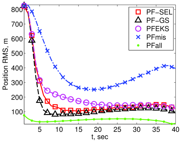
(a) Position RMSE versus time

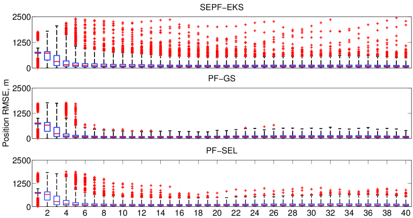
(b) Boxplots of position RMSEs versus time (seconds)

Figure 1: Tracking performance of the particle filters as a function of time using RMS error as a performance metric. (a) The curves show the means of 5000 Monte-Carlo trials. (b) Errorbars showing the variation of position RMS for SEPF-EKS, PF-GS and PF-SEL, when they use 2000 particles. The box has lines at the lower quartile, median(red line), and upper quartile values. Outliers (red ’+’) are values beyond the range of 5 times the interquartile range from the ends of the box.

VII-A Benchmarked Filters

We have implemented five different particle filters, all based on the Sampling Importance Resampling (SIR) filtering paradigm [24]. The prior distribution is used as the importance function. The filters were implemented in Matlab and the code was highly optimized.

PFall: collects all measurements from all active sensors (no OOSMs). This is an idealized filter that provides a performance benchmark; a real-time implementation is impossible.

PFmis: discards all OOSMs and therefore only processes the measurements with zero delay.

SEPF-EKS: Storage efficient particle filter using EKS smoothing as described in [15] (Algorithm 3).

PF-GS: The OOSM-GARP algorithm described in Algorithm 2.

PF-SEL: Selective OOSM processing based on the proposed framework and described in Algorithm 5.

We use the root mean-squared (RMS) position error to compare the performances of the particle filters. Let $({p_{k}^{x}},{p_{k}^{y}})$ and $(\hat{p}_{k,i}^{x},\hat{p}_{k,i}^{y})$ denote the true and estimated target positions at time step $k$ for the $i$-th of $M$ Monte-Carlo runs. The RMS position error at $k$ is calculated as

$$\textrm{RMS}_{k}=\sqrt{\frac{1}{M}\sum_{i=1}^{M}(\hat{p}_{k,i}^{x}-{p_{k}^{x}})^{2}+(\hat{p}_{k,i}^{y}-{p_{k}^{y}})^{2}}$$ (43)

VII-B Results and Discussion

In our first experiment we fix the computational cost $C_{\mathrm{ave}}=0.6$. We thus allow $0.6$ sweeps of the SEPF-EKS algorithm to be performed on average per filtering step. Over an extended period of time of sufficiently large length $L$ this leads to an additional OOSM processing overhead of $\sim 0.6LC_{EKS}$ where $C_{EKS}$ is the cost of one sweep of the SEPF-EKS algorithm. If we do not apply the proposed procedure and process all the available OOSMs this cost in our application scenario is approximately $1.5LC_{EKS}$. This implies that we process only approximately $40\%$ of all measurements.

In Fig. 1, we plot the respective RMS position performance for the tracking period of $40s$ for the algorithms with these settings. Corresponding error-bar plots of the RMS performance are shown in Fig. 1(b). The actual number of individual OOSMs processed by the SEPF-EKS after application of the first threshold $\gamma_{k}$ measured in our experiment is $40.04\%$. After the second threshold $\nu=1/40$ the percentage of most informative OOSMs processed by rerunning the particle filter using OOSM-GARP is $1.57\%$.

Fig. 1 indicates that despite processing only a relatively small fraction of the OOSMs, the proposed algorithm performs almost as well as the much more complex OOSM-GARP algorithm (PF-GS). The calculation of the selection criterion has minimal overhead, so discarding the uninformative measurements results in significant computational savings. Thus the proposed filter is more computationally efficient than the SEPF-EKS filter and yet, as can be seen from Fig. 1, it has better RMS performance. Fig. 1(b) indicates that the performance of SEPF-EKS is not as stable as that of PF-GS and PF-SEL. In the proposed algorithm the increased robustness and performance stability is achieved by using the second threshold to detect situations when reweighting particles induces sample degeneracy problems.

In our next experiment we study the computational complexity versus accuracy trade-off for the proposed algorithm. We illustrate this by varying the computational complexity of the proposed algorithm by adjusting $C_{\mathrm{ave}}$ and plotting the RMS error vs. computational load measured in MATLAB. We use the following values to control the OOSM processing overhead: $C_{\mathrm{ave}}=\{0,0.1,0.2,0.4,0.5,0.6,0.8,1,1.3,2\}$, $\gamma_{2}=1/40$. These results are reported in Fig. 2. In this figure we show the relationship between complexity and performance for the proposed algorithm with ten values of $C_{\mathrm{ave}}$ and results of 10 simulations for other algorithms. Each simulation involves 1000 Monte Carlo runs. We compare the performance of all particle filters when they use $2000$ particles; qualitatively similar results were observed for $1000$ and $5000$ particles. When the thresholds are chosen so that the proposed filter has the same computational complexity as SEPF-EKS, it achieves significantly better tracking performance. Alternatively, for the same fixed RMS error performance, the selective processing algorithm reduces the computational load by $30-40\%$. Compared to the OOSM-GARP algorithm, a $50\%$ reduction in computational requirements leads to only a small increase in estimation error. The results illustrate that we can adjust $C_{\mathrm{ave}}$ to control the trade-off between the average computational load or power supply consumption and the tracking performance.

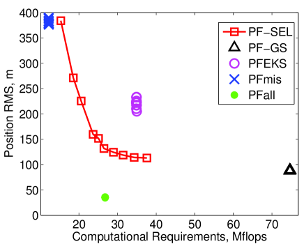
(a) $N=2000$, $t=10$

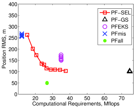
(b) $N=2000$, $t=20$

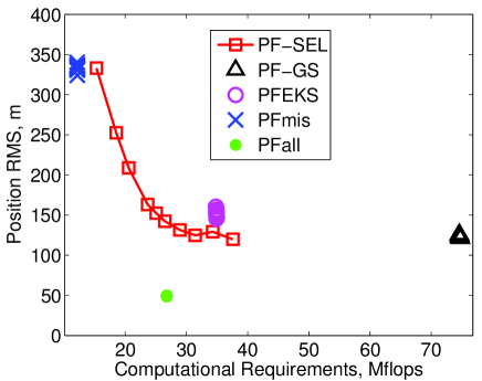
(c) $N=2000$, $t=30$

Figure 2: RMS vs Complexity from $10$ simulations with different $C_{\mathrm{ave}}$. Each simulation shows the average of $1000$ MC runs.We select three timesteps, $t=10,20,30$ for filters with $2000$ and $5000$ particles. The complexity is measured by running time for tracking $40$s of each filter. The results are run on a Dell laptop with Genuine Intel(R) CPU T2400 1.83GHz, 0.99GB RAM and Win-XP OS.

VIII Conclusions

This paper presents a framework for selective processing of the out-of-sequence measurements. Based on this framework we develop a computationally efficient algorithm for delay-tolerant particle filtering that has limited memory requirements. By identifying and discarding the uninformative delayed measurements, the algorithm reduces the computational requirements. By processing the most informative measurements with a re-run particle filter, the algorithm achieves better tracking performance than the storage efficient particle filter of [15].

In our framework, the threshold to discard uninformative measurements is set by minimizing the one-step MSE calculated from the Gaussian approximation of posterior at every filtering time instant. The threshold setting could be improved by employing a finite horizon dynamic programming technique to take into account the MSE reduction over several forthcoming steps. It is also interesting to explore whether the fusion centre can provide feedback to the sensor nodes so that they can locally assess measurement informativeness. This would allow sensor nodes to avoid unnecessary energy expenditure by discarding uninformative measurements prior to transmission.

Appendix A Proof of Theorem 1

We here provide a proof of Theorem 1.

We first state a lemma that is employed within the main proof. Denote the spectral radius of a matrix by $\rho(\cdot)=\max_{i}|\lambda_{i}(\cdot)|$. The proof of the lemma involves expanding the variational characterization of the spectral radius in terms of the blocks of ${\mathbf{A}}$ and applying the Cauchy-Schwarz inequality to each term in the expansion.

Lemma 1.

Let ${\mathbf{A}}\in\mathbb{R}^{K\times K}$ be a block matrix consisting of blocks ${\mathbf{A}}_{i,j}\in\mathbb{R}^{K_{i}\times M_{j}}$. Then $\rho({\mathbf{A}})\leq\sum_{i,j}\rho({\mathbf{A}}_{i,j}^{T}{\mathbf{A}}_{i,j})^{1/2}$.

Proof:

Let $\{{\mathbf{x}}_{i}\}$ and $\{{\mathbf{y}}_{j}\}$ be two partitionings of vector ${\mathbf{X}}\in\mathbb{R}^{K}$ such that ${\mathbf{X}}^{T}=[{\mathbf{x}}_{1}^{T},{\mathbf{x}}_{2}^{T},\ldots]$, ${\mathbf{x}}_{i}\in\mathbb{R}^{K_{i}},\forall i$ and ${\mathbf{X}}^{T}=[{\mathbf{y}}_{1}^{T},{\mathbf{y}}_{2}^{T},\ldots]$, ${\mathbf{y}}_{j}\in\mathbb{R}^{M_{j}},\forall j$. Write the variational characterization of the spectral radius and expand it in terms of blocks:

$$\rho({\mathbf{A}}) =\max_{{\mathbf{X}}\neq 0}\frac{|{\mathbf{X}}^{T}{\mathbf{A}}{\mathbf{X}}|}{{\mathbf{X}}^{T}{\mathbf{X}}}$$ (44)

$$=\max_{{\mathbf{X}}\neq 0}\frac{|\sum_{i,j}{\mathbf{x}}_{i}^{T}{\mathbf{A}}_{i,j}{\mathbf{y}}_{j}|}{{\mathbf{X}}^{T}{\mathbf{X}}}$$ (45)

$$\leq\max_{{\mathbf{X}}\neq 0}\frac{\sum_{i,j}|{\mathbf{x}}_{i}^{T}{\mathbf{A}}_{i,j}{\mathbf{y}}_{j}|}{{\mathbf{X}}^{T}{\mathbf{X}}}$$ (46)

$$\leq\sum_{i,j}\max_{{\mathbf{X}}\neq 0}\frac{|{\mathbf{x}}_{i}^{T}{\mathbf{A}}_{i,j}{\mathbf{y}}_{j}|}{{\mathbf{X}}^{T}{\mathbf{X}}}.$$ (47)

Now, for every summand use the Cauchy-Schwarz inequality and take into account the fact that ${\mathbf{x}}_{i}^{T}{\mathbf{x}}_{i}/{\mathbf{X}}^{T}{\mathbf{X}}\leq 1,\forall i$:

$$\max_{{\mathbf{X}}\neq 0}\frac{|{\mathbf{x}}_{i}^{T}{\mathbf{A}}_{i,j}{\mathbf{y}}_{j}|}{{\mathbf{X}}^{T}{\mathbf{X}}} \leq\max_{{\mathbf{X}}\neq 0}\frac{|{\mathbf{x}}_{i}^{T}{\mathbf{x}}_{i}|^{1/2}}{|{\mathbf{X}}^{T}{\mathbf{X}}|^{1/2}}\frac{|{\mathbf{y}}_{j}^{T}{\mathbf{A}}_{i,j}^{T}{\mathbf{A}}_{i,j}{\mathbf{y}}_{j}|^{1/2}}{|{\mathbf{X}}^{T}{\mathbf{X}}|^{1/2}}$$ (48)

$$\leq\max_{{\mathbf{X}}\neq 0}\frac{|{\mathbf{y}}_{j}^{T}{\mathbf{A}}_{i,j}^{T}{\mathbf{A}}_{i,j}{\mathbf{y}}_{j}|^{1/2}}{|{\mathbf{X}}^{T}{\mathbf{X}}|^{1/2}}.$$ (49)

Similarly, note the fact that ${\mathbf{y}}_{j}^{T}{\mathbf{y}}_{j}\leq{\mathbf{X}}^{T}{\mathbf{X}},\forall j$:

$$\max_{{\mathbf{X}}\neq 0}\frac{|{\mathbf{y}}_{j}^{T}{\mathbf{A}}_{i,j}^{T}{\mathbf{A}}_{i,j}{\mathbf{y}}_{j}|^{1/2}}{|{\mathbf{X}}^{T}{\mathbf{X}}|^{1/2}} \leq\max_{{\mathbf{X}}\neq 0}\frac{|{\mathbf{y}}_{j}^{T}{\mathbf{A}}_{i,j}^{T}{\mathbf{A}}_{i,j}{\mathbf{y}}_{j}|^{1/2}}{|{\mathbf{y}}_{j}^{T}{\mathbf{y}}_{j}|^{1/2}}$$ (50)

$$=\left(\max_{{\mathbf{y}}_{j}\neq 0}\frac{|{\mathbf{y}}_{j}^{T}{\mathbf{A}}_{i,j}^{T}{\mathbf{A}}_{i,j}{\mathbf{y}}_{j}|}{|{\mathbf{y}}_{j}^{T}{\mathbf{y}}_{j}|}\right)^{1/2}.$$ (51)

This is the variational characterization of $\rho({\mathbf{A}}_{i,j}^{T}{\mathbf{A}}_{i,j})^{1/2}$. Substituting it into (44) completes the proof. ∎

Proof:

Employing the EKF linear approximation in (10) and using the independence of measurement and diffusion noises from each other and from the state and independence of $\zeta_{m}^{s}$ and $\zeta_{n}^{j}$ for any $m\neq n$ or $s\neq j$, we have for $m>n$ and any $s,j$:

$${\mathbf{R}}_{Y_{m}^{s}Y_{n}^{j}} ={\mathbf{H}}_{m}^{s}{\mathbf{F}}_{m,n}{\mathbf{R}}_{X_{n}X_{n}}{{\mathbf{H}}_{n}^{j}}^{T}$$ (52)

Note that for $m<n$ ${\mathbf{R}}_{Y_{m}^{s}Y_{n}^{j}}={\mathbf{R}}_{Y_{n}^{s}Y_{m}^{j}}^{T}={\mathbf{H}}_{m}^{s}{\mathbf{R}}_{X_{m}X_{m}}{\mathbf{F}}_{n,m}^{T}{{\mathbf{H}}_{n}^{j}}^{T}$.

Recall that ${\mathbf{B}}_{\mathcal{Z}_{k}\mathcal{Z}_{k}}$ is the block-diagonal matrix whose blocks match the diagonal blocks of ${\mathbf{R}}_{\mathcal{Z}_{k}\mathcal{Z}_{k}}$. We now establish finite upper bounds on two spectral radii, $\rho({\mathbf{B}}_{\mathcal{Z}_{k}\mathcal{Z}_{k}}-{\mathbf{R}}_{\mathcal{Z}_{k}\mathcal{Z}_{k}})$ and $\rho({\mathbf{R}}_{X_{k}\mathcal{Z}_{k}}{\mathbf{R}}_{\mathcal{Z}_{k}X_{k}})$. Throughout the proof we employ the fact that $\rho({\mathbf{C}}^{T}{\mathbf{A}}{\mathbf{C}})\leq\rho({\mathbf{A}})\rho({\mathbf{C}}^{T}{\mathbf{C}})$ for a square matrix ${\mathbf{A}}$ and an arbitrary real matrix ${\mathbf{C}}$. This follows from the variational characterization of spectral radius:

$$\rho({\mathbf{C}}^{T}{\mathbf{A}}{\mathbf{C}}) =\max_{{\mathbf{x}}\neq 0}\frac{|{\mathbf{x}}^{T}{\mathbf{C}}^{T}{\mathbf{A}}{\mathbf{C}}{\mathbf{x}}|}{{\mathbf{x}}^{T}{\mathbf{x}}}=\max_{{\mathbf{x}}\neq 0}\left(\frac{|{\mathbf{x}}^{T}{\mathbf{C}}^{T}{\mathbf{A}}{\mathbf{C}}{\mathbf{x}}|}{{\mathbf{x}}^{T}{\mathbf{C}}^{T}{\mathbf{C}}{\mathbf{x}}}\frac{{\mathbf{x}}^{T}{\mathbf{C}}^{T}{\mathbf{C}}{\mathbf{x}}}{{\mathbf{x}}^{T}{\mathbf{x}}}\right)$$ (53)

$$\leq\max_{{\mathbf{x}}\neq 0}\left(\max_{{\mathbf{y}}\neq 0}\frac{|{\mathbf{y}}^{T}{\mathbf{A}}{\mathbf{y}}|}{{\mathbf{y}}^{T}{\mathbf{y}}}\frac{{\mathbf{x}}^{T}{\mathbf{C}}^{T}{\mathbf{C}}{\mathbf{x}}}{{\mathbf{x}}^{T}{\mathbf{x}}}\right)$$ (54)

$$\leq\rho({\mathbf{A}})\rho({\mathbf{C}}^{T}{\mathbf{C}}),$$ (55)

Since all the diagonal blocks of ${\mathbf{B}}_{\mathcal{Z}_{k}\mathcal{Z}_{k}}-{\mathbf{R}}_{\mathcal{Z}_{k}\mathcal{Z}_{k}}$ are zero, we have from Lemma 1 and (52):

$$\rho( {\mathbf{B}}_{\mathcal{Z}_{k}\mathcal{Z}_{k}}-{\mathbf{R}}_{\mathcal{Z}_{k}\mathcal{Z}_{k}})$$

$$\leq\sum_{m=k-\ell}^{k-1}\sum_{s\in\mathcal{S}_{m,k}}\left(\sum_{n=k-\ell,n\neq m}^{k-1}\sum_{j\in\mathcal{S}_{n,k}}\rho({\mathbf{R}}_{Y_{m}^{s}Y_{n}^{j}}{\mathbf{R}}_{Y_{n}^{j}Y_{m}^{s}})^{1/2}+\sum_{j\in\mathcal{S}_{m,k},j\neq s}\rho({\mathbf{R}}_{Y_{m}^{s}Y_{m}^{j}}{\mathbf{R}}_{Y_{m}^{j}Y_{m}^{s}})^{1/2}\right)$$

$$\leq K\ell(K\ell-1)\max_{s,m}\max_{j\neq s\vee n\neq m}\rho({\mathbf{R}}_{Y_{m}^{s}Y_{n}^{j}}{\mathbf{R}}_{Y_{n}^{j}Y_{m}^{s}})^{1/2}$$

$$\leq K\ell(K\ell-1)\max_{s,m}\max_{j\neq s\vee n\neq m}\max[\rho({\mathbf{H}}_{m}^{s}{\mathbf{F}}_{m,n}{\mathbf{R}}_{X_{n}X_{n}}{{\mathbf{H}}_{n}^{j}}^{T}{{\mathbf{H}}_{n}^{j}}{\mathbf{R}}_{X_{n}X_{n}}{\mathbf{F}}_{m,n}^{T}{{\mathbf{H}}_{m}^{s}}^{T})^{1/2},$$

$$\quad\quad\quad\rho({\mathbf{H}}_{n}^{j}{\mathbf{F}}_{n,m}{\mathbf{R}}_{X_{m}X_{m}}{{\mathbf{H}}_{m}^{s}}^{T}{{\mathbf{H}}_{m}^{j}}{\mathbf{R}}_{X_{m}X_{m}}{\mathbf{F}}_{n,m}^{T}{{\mathbf{H}}_{n}^{j}}^{T})^{1/2}]$$

$$\leq K\ell(K\ell-1)\max_{n}\rho({\mathbf{R}}_{X_{n}X_{n}})\max_{s,m}\rho({\mathbf{H}}_{m}^{s}{{\mathbf{H}}_{m}^{s}}^{T})^{1/2}\max_{s,m}\rho({{\mathbf{H}}_{m}^{s}}^{T}{\mathbf{H}}_{m}^{s})^{1/2}\max_{n\leq m}\rho({\mathbf{F}}_{m,n}{\mathbf{F}}_{m,n}^{T})^{1/2}$$ (56)

Observing that ${\mathbf{R}}_{X_{k}\mathcal{Z}_{k}}{\mathbf{R}}_{\mathcal{Z}_{k}X_{k}}=\sum_{s,m}{\mathbf{R}}_{X_{k}Y_{m}^{s}}{\mathbf{R}}_{X_{k}Y_{m}^{s}}^{T}$ and recalling (33) we can write:

$$\rho({\mathbf{R}}_{X_{k}\mathcal{Z}_{k}}{\mathbf{R}}_{\mathcal{Z}_{k}X_{k}}) \leq\sum_{s,m}\rho({\mathbf{R}}_{X_{k}Y_{m}^{s}}{\mathbf{R}}_{X_{k}Y_{m}^{s}}^{T})$$ (57)

$$\leq K\ell\max_{s,m}\rho({\mathbf{F}}_{k,m}{\mathbf{F}}_{k,m}^{T})\rho({{\mathbf{H}}_{m}^{s}}^{T}{{\mathbf{H}}_{m}^{s}})\rho({\mathbf{R}}_{X_{m}X_{m}})^{2}.$$ (58)

Assumptions $\mathcal{A}_{1}$-$\mathcal{A}_{3}$ ensure that the bounds in (A) and (57) are finite.

We now develop an upper bound for $\rho({\mathbf{R}}_{\mathcal{Z}_{k}\mathcal{Z}_{k}}^{-1}-{\mathbf{B}}_{\mathcal{Z}_{k}\mathcal{Z}_{k}}^{-1})$

$$\rho({\mathbf{R}}_{\mathcal{Z}_{k}\mathcal{Z}_{k}}^{-1}-{\mathbf{B}}_{\mathcal{Z}_{k}\mathcal{Z}_{k}}^{-1}) =\rho({\mathbf{R}}_{\mathcal{Z}_{k}\mathcal{Z}_{k}}^{-1}({\mathbf{B}}_{\mathcal{Z}_{k}\mathcal{Z}_{k}}-{\mathbf{R}}_{\mathcal{Z}_{k}\mathcal{Z}_{k}}){\mathbf{B}}_{\mathcal{Z}_{k}\mathcal{Z}_{k}}^{-1})$$

$$\leq\rho({\mathbf{R}}_{\mathcal{Z}_{k}\mathcal{Z}_{k}}^{-1})\rho({\mathbf{B}}_{\mathcal{Z}_{k}\mathcal{Z}_{k}}-{\mathbf{R}}_{\mathcal{Z}_{k}\mathcal{Z}_{k}})\rho({\mathbf{B}}_{\mathcal{Z}_{k}\mathcal{Z}_{k}}^{-1})$$

$$=\lambda_{\min}^{-1}({\mathbf{R}}_{\mathcal{Z}_{k}\mathcal{Z}_{k}})\lambda_{\min}^{-1}({\mathbf{B}}_{\mathcal{Z}_{k}\mathcal{Z}_{k}})\rho({\mathbf{B}}_{\mathcal{Z}_{k}\mathcal{Z}_{k}}-{\mathbf{R}}_{\mathcal{Z}_{k}\mathcal{Z}_{k}}).$$ (59)

Since the eigenvalues of the block-diagonal matrix are the eigenvalues of its blocks we have: $\lambda_{\min}({\mathbf{B}}_{\mathcal{Z}_{k}\mathcal{Z}_{k}})=\min_{s,m}\lambda_{\min}({\mathbf{R}}_{Y_{m}^{s}Y_{m}^{s}})$. This implies:

$$\lambda_{\min}({\mathbf{B}}_{\mathcal{Z}_{k}\mathcal{Z}_{k}}) =\min_{s,m}\lambda_{\min}({\mathbf{H}}_{m}^{s}{\mathbf{R}}_{X_{m}X_{m}}{{\mathbf{H}}_{m}^{s}}^{T}+{\mathbf{R}}_{\zeta_{m}^{s}\zeta_{m}^{s}})$$

$$\geq\min_{s,m}\lambda_{\min}({\mathbf{R}}_{\zeta_{m}^{s}\zeta_{m}^{s}}).$$ (60)

The last inequality holds because (i) for any matrices ${\mathbf{A}}$ and ${\mathbf{C}}$ $\lambda_{\min}({\mathbf{A}}+{\mathbf{C}})\geq\lambda_{\min}({\mathbf{A}})+\lambda_{\min}({\mathbf{C}})$ and (ii) ${{\mathbf{H}}_{m}^{s}}{\mathbf{R}}_{X_{m}X_{m}}{{\mathbf{H}}_{m}^{s}}^{T}$ is positive semidefinite.

Similarly, since ${\mathbf{R}}_{\mathcal{Z}_{k}\mathcal{Z}_{k}}$ is a covariance matrix and as such is positive semidefinite we deduce:

$$\lambda_{\min}({\mathbf{R}}_{\mathcal{Z}_{k}\mathcal{Z}_{k}}) =\lambda_{\min}({\mathbf{B}}_{\mathcal{Z}_{k}\mathcal{Z}_{k}}+({\mathbf{R}}_{\mathcal{Z}_{k}\mathcal{Z}_{k}}-{\mathbf{B}}_{\mathcal{Z}_{k}\mathcal{Z}_{k}}))$$ (61)

$$\geq\max[0,\lambda_{\min}({\mathbf{B}}_{\mathcal{Z}_{k}\mathcal{Z}_{k}})+\lambda_{\min}({\mathbf{R}}_{\mathcal{Z}_{k}\mathcal{Z}_{k}}-{\mathbf{B}}_{\mathcal{Z}_{k}\mathcal{Z}_{k}})]$$ (62)

$$\geq\min_{s,m}\lambda_{\min}({\mathbf{R}}_{\zeta_{m}^{s}\zeta_{m}^{s}})-\rho({\mathbf{B}}_{\mathcal{Z}_{k}\mathcal{Z}_{k}}-{\mathbf{R}}_{\mathcal{Z}_{k}\mathcal{Z}_{k}})$$ (63)

The last line is valid provided $\min_{s,m}\lambda_{\min}({\mathbf{R}}_{\zeta_{m}^{s}\zeta_{m}^{s}})>\rho({\mathbf{B}}_{\mathcal{Z}_{k}\mathcal{Z}_{k}}-{\mathbf{R}}_{\mathcal{Z}_{k}\mathcal{Z}_{k}})$, which holds for sufficiently large $\lambda_{\min}$ due to the finite bound derived for the spectral radius in (A).

We can now derive the following bound on the expression of interest in the theorem, employing the relationship $\operatorname{tr}(\cdot)=\sum_{i}\lambda_{i}(\cdot)$:

$$|\operatorname{tr}{\mathbf{R}}_{X_{k}\mathcal{Z}_{k}}{\mathbf{R}}_{\mathcal{Z}_{k}\mathcal{Z}_{k}}^{-1}{\mathbf{R}}_{\mathcal{Z}_{k}X_{k}} -\operatorname{tr}{\mathbf{R}}_{X_{k}\mathcal{Z}_{k}}{\mathbf{B}}_{\mathcal{Z}_{k}\mathcal{Z}_{k}}^{-1}{\mathbf{R}}_{\mathcal{Z}_{k}X_{k}}|$$ (64)

$$=|\operatorname{tr}{\mathbf{R}}_{X_{k}\mathcal{Z}_{k}}({\mathbf{R}}_{\mathcal{Z}_{k}\mathcal{Z}_{k}}^{-1}-{\mathbf{B}}_{\mathcal{Z}_{k}\mathcal{Z}_{k}}^{-1}){\mathbf{R}}_{\mathcal{Z}_{k}X_{k}}|$$ (65)

$$\leq K\ell\rho({\mathbf{R}}_{X_{k}\mathcal{Z}_{k}}({\mathbf{R}}_{\mathcal{Z}_{k}\mathcal{Z}_{k}}^{-1}-{\mathbf{B}}_{\mathcal{Z}_{k}\mathcal{Z}_{k}}^{-1}){\mathbf{R}}_{\mathcal{Z}_{k}X_{k}}),$$ (66)

$$\leq K\ell\rho({\mathbf{R}}_{\mathcal{Z}_{k}\mathcal{Z}_{k}}^{-1}-{\mathbf{B}}_{\mathcal{Z}_{k}\mathcal{Z}_{k}}^{-1})\rho({\mathbf{R}}_{X_{k}\mathcal{Z}_{k}}{\mathbf{R}}_{\mathcal{Z}_{k}X_{k}}),$$ (67)

$$\leq K\ell\lambda_{\min}^{-1}({\mathbf{R}}_{\mathcal{Z}_{k}\mathcal{Z}_{k}})\lambda_{\min}^{-1}({\mathbf{B}}_{\mathcal{Z}_{k}\mathcal{Z}_{k}})\rho({\mathbf{B}}_{\mathcal{Z}_{k}\mathcal{Z}_{k}}-{\mathbf{R}}_{\mathcal{Z}_{k}\mathcal{Z}_{k}})\rho({\mathbf{R}}_{X_{k}\mathcal{Z}_{k}}{\mathbf{R}}_{\mathcal{Z}_{k}X_{k}}),$$ (68)

$$\leq\frac{K\ell\rho({\mathbf{R}}_{X_{k}\mathcal{Z}_{k}}{\mathbf{R}}_{\mathcal{Z}_{k}X_{k}})\rho({\mathbf{B}}_{\mathcal{Z}_{k}\mathcal{Z}_{k}}-{\mathbf{R}}_{\mathcal{Z}_{k}\mathcal{Z}_{k}})}{(\min_{s,m}\lambda_{\min}({\mathbf{R}}_{\zeta_{m}^{s}\zeta_{m}^{s}})-\rho({\mathbf{B}}_{\mathcal{Z}_{k}\mathcal{Z}_{k}}-{\mathbf{R}}_{\mathcal{Z}_{k}\mathcal{Z}_{k}}))\min_{s,m}\lambda_{\min}({\mathbf{R}}_{\zeta_{m}^{s}\zeta_{m}^{s}})}.$$ (69)

The finite bounds on the expressions in the numerator lead us to the conclusion that $\min_{s,m}\lambda_{\min}({\mathbf{R}}_{\zeta_{m}^{s}\zeta_{m}^{s}})\rightarrow\infty\Rightarrow|\operatorname{tr}{\mathbf{R}}_{X_{k}\mathcal{Z}_{k}}{\mathbf{R}}_{\mathcal{Z}_{k}\mathcal{Z}_{k}}^{-1}{\mathbf{R}}_{\mathcal{Z}_{k}X_{k}}-\operatorname{tr}{\mathbf{R}}_{X_{k}\mathcal{Z}_{k}}{\mathbf{B}}_{\mathcal{Z}_{k}\mathcal{Z}_{k}}^{-1}{\mathbf{R}}_{\mathcal{Z}_{k}X_{k}}|\rightarrow 0$, completing the proof.

∎

References

• [1] R. D. Hilton, D. A. Martin, and W. D. Blair, “Tracking with time-delayed data in multisensor systems,” Naval Surface Warfare Center, Dahlgren,VA, Tech. Rep. NSWCD/TR-93/351, August 1993.
• [2] M. Mallick, S. Coraluppi, and C. Carthel, “Advances in asynchronous and decentralized estimation,” in Proc. IEEE Aerospace Conf., vol. 4, Mar. 2001, pp. 1873–1888.
• [3] Y. Bar-Shalom, “Update with out-of-sequence measurements in tracking: Exact solution,” IEEE Trans. Aerosp. Electron. Syst., vol. 38, no. 3, pp. 769–778, Mar. 2002.
• [4] S. Challa, R. J. Evans, and X. Wang, “A Bayesian solution and its approximations to out-of-sequence measurement problems,” Information Fusion, vol. 4, no. 3, pp. 185 – 199, 2003.
• [5] Y. Bar-Shalom, H. Chen, and M. Mallick, “One-step solution for the multistep out-of-sequence-measurement problem in tracking,” IEEE Trans. Aerosp. Electron. Syst., vol. 40, no. 1, pp. 27–37, Jan. 2004.
• [6] K. Zhang, X. Li, and Y. Zhu, “Optimal update with out-of-sequence measurements,” IEEE Trans. Signal Process., vol. 53, no. 6, pp. 1992–2004, June 2005.
• [7] S. R. Maskell, R. G. Everitt, R. Wright, and M. Briers, “Multi-target out-of-sequence data association: Tracking using graphical models,” Information Fusion, vol. 7, no. 4, pp. 434 – 447, Dec. 2006.
• [8] X. Shen, Y. Zhu, E. Song, and Y. Luo, “Optimal centralized update with multiple local out-of-sequence measurements,” IEEE Trans. Signal Process., vol. 57, no. 4, pp. 1551–1562, Apr. 2009.
• [9] S. Zhang, Y. Bar-Shalom, and G. Watson, “Tracking with multisensor out-of-sequence measurements with residual biases,” in Proc. ISIF Int. Conf. Information Fusion,, Edinburgh, UK, Jul. 2010.
• [10] M. Orton and A. Marrs, “Storage efficient particle filters for the out of sequence measurement problem,” in Proc. IEE Colloqium on Target Tracking: Algorithms and Applications, Enschede, The Netherlands, Oct. 2001.
• [11] ——, “Particle filters for tracking with out-of-sequence measurements,” IEEE Trans. Aerosp. Electron. Syst., vol. 41, no. 2, pp. 693–702, Feb. 2005.
• [12] M. Mallick, T. Kirubarajan, and S. Arulampalam, “Out-of-sequence measurement processing for tracking ground target using particle filters,” in Proc. IEEE Aerospace Conf., vol. 4, Mar. 2002, pp. 1809–1818.
• [13] W. Zhang, X. Huang, and M. Wang, “Out-of-sequence measurement algorithm based on Gaussian particle filter,” Information Technology Journal, vol. 9, no. 5, pp. 942–948, May 2010.
• [14] J. Kotecha and P. Djuric, “Gaussian particle filtering,” IEEE Trans. Signal Process., vol. 51, no. 10, pp. 2592 – 2601, Oct. 2003.
• [15] U. Orguner and F. Gustafsson, “Storage efficient particle filters for the out of sequence measurement problem,” in Proc. ISIF Int. Conf. Information Fusion, Cologne, Germany, July 2008.
• [16] P. Fearnhead, D. Wyncoll, and J. Tawn, “A sequential smoothing algorithm with linear computational cost,” Biometrika, vol. 97, no. 2, pp. 447–464, June 2010.
• [17] M. Briers, A. Doucet, and S. Maskell, “Smoothing algorithms for state–space models,” Annals of the Institute of Statistical Mathematics, vol. 62, no. 1, pp. 61–89, Feb. 2010.
• [18] D. K. Tasoulis, N. M. Adams, and D. J. Hand, “Selective fusion of out-of-sequence measurements,” Information Fusion, vol. 11, no. 2, pp. 183 – 191, Apr. 2010.
• [19] X. Liu, B. N. Oreshkin, and M. J. Coates, “Efficient delay-tolerant particle filtering through selective processing of out-of-sequence measurements,” in Proc. ISIF Int. Conf. Information Fusion, Edinburgh, UK, Jul. 2010.
• [20] K. K. Biswas and A. Mahalana, “Suboptimal algorithms for nonlinear smoothing,” IEEE Trans. Aerosp. Electron. Syst., vol. 9, no. 4, pp. 529–534, Apr. 1973.
• [21] H. E. Rauch, F. Tung, and C. Striebel, “Maximum likelihood estimates of linear dynamic systems,” AIAA, vol. 3, no. 8, pp. 1445–50, Aug 1965.
• [22] R. Horn and C. Johnson, Matrix analysis.   Cambridge Univ Pr, 1990.
• [23] Y. Bar-Shalom, X. R. Li, and T. Kirubarajan, Estimation with Applications to Tracking and Navigation, 1st ed.   Wiley-Interscience, Jun. 2001.
• [24] N. J. Gordon, D. J. Salmond, and A. F. M. Smith, “Novel approach to nonlinear/non-Gaussian Bayesian state estimation,” Radar and Signal Processing, IEEE Proceedings F, vol. 140, no. 2, pp. 107–113, Apr. 1993.