Lattice String Field Theory

Abstract:

String field theory is a candidate for a full non-perturbative definition of string theory. We aim to define string field theory on a space-time lattice to investigate its behaviour at the quantum level. Specifically, we look at string field theory in a one dimensional linear dilaton background. We report the first results of our simulations.

1 Introduction

Superstring theory is currently the most promising candidate for a theory of everything. Yet, it is not clear what superstring theory is. Moreover, even the perturbation theory of the standard (RNS) formulation of string theory is not yet completely established beyond some loop level, due to complications related to supermoduli spaces [1, 2, 3]. A possible way to define superstring theory that might also resolve the problems with supermoduli spaces, is as a superstring field theory, i.e., as a field theory of strings (see [4] for a recent review). It is natural to expect from a reliable formulation of superstring field theory that it respects the underlying symmetries of string theory, i.e., it should be covariant and, moreover, universal [5]. There are several variants of superstring field theories of this kind, e.g., the heterotic [6] and open [7, 8, 9, 10] theories. However, it was never checked if any of those is really well defined at the quantum level. It is our intention to address this question using lattice techniques.

Some of the formulations of superstring field theory cannot be expected, at this stage, to be consistent at the quantum level, since, e.g., they don’t include a consistent Ramond sector. The fermions of the Ramond sector, as well as the notion of “picture” [11] introduce, in any case, some complications for the theory. Hence, it might be advisable to start with a simpler model, such as that of the bosonic string. The bosonic closed string field theory [12] is much more complicated than the open one [13]. Hence, we concentrate on the later.

It is known that the bosonic string theory is consistent in flat space only in 26 dimensions. Simulating any theory on a 26 dimensional lattice is almost a hopeless task. Moreover, the theory has tachyons, both in the open and in the closed string spectrum. It is by now understood that the open string tachyon is related to a condensation of an unstable D-brane [5, 14, 15, 16]. However, no analogous understanding exists regarding the fate of the closed string tachyon [17, 18, 19]. Both problems can be avoided by considering “non-critical” string theory. The non-critical theory lives at lower dimensions and for $d\leq 2$ the tachyon is absent. On the other hand, a new complication is introduced, namely the theory includes a linear dilaton, which breaks Poincaré invariance. Moreover, all the coupling constants are proportional to the dilaton vacuum expectation value, which runs to infinity in one direction. These issues pose a challenge to a lattice simulation.

A simple consideration of world-sheet gauge symmetry and degrees of freedom reveals that two of the $d$ dimensions in which the string lives are unphysical. Indeed, the two-dimensional string theory is already not a string theory, but a field theory, in the sense that only one physical field out of the infinitely many ones, remains. This field is the “tachyon”, which is now a massless field. Going on to “lower dimensions” is possible. The dimension is replaced by the central charge of the conformal field theory. This is natural, since $d$ flat dimensions correspond to $c=d$, where $c$ is the central charge. The two-dimensional theory includes a single flat scalar field, i.e., a $c=1$ system, coupled to a single linear dilaton direction. Theories with $0\leq c<1$ exist and are well studied. They go under the name of “minimal models” [20, 21]. For simplicity we are starting this study with the simplest model of all, the $c=0$ theory that includes only the one dimensional linear dilaton direction with $c=26$ and the canonical ghost system with $c=-26$.

While minimal models have only a finite number of degrees of freedom, the string field theory that describe them still contains an infinite number of fields. Almost all of the degrees of freedom of the theory should then be removed by the very large gauge symmetry present. This fact raises two further problem that one should address. First, we have to truncate the infinite number of fields to a finite number while taking this number to infinity eventually. Second, we have to address the existence of the gauge symmetry. The first issue of “level truncation” was much employed in the string field theory literature [22, 23, 24], albeit only at the classical level. It is not even a-priori clear that it would be a consistent regularization at the quantum level. Here, we apply an “experimental approach” towards this question. The issue of gauge symmetry arises only at the next level. Since in this report we only concentrate on preliminary results from the lowest level, we ignore this issue for now.

2 Methods

The “level” of level truncation is, up to an additive constant, the eigenvalue of the “Hamiltonian” $L_{0}$ (the zeroth Virasoro generator). As such, the level includes two contributions, that of the field itself, which is different for any of the infinitely many fields of which the string field is composed and a momentum contribution for each possible mode of the field. The former contribution is denoted $l_{0}$ and the total level is given by,

$$l=l_{0}+\alpha^{\prime}p^{2}\,,$$ (1)

where $p$ is the momentum and $\alpha^{\prime}$ is a dimensional constant setting the string scale. We also assumed that the fields were properly redefined, e.g., instead of the canonical “tachyon field” $T(x)$ we consider $\tau(x)=e^{-\frac{Vx}{2}}T(x)$. This is the only field with $l_{0}=0$.

The $l_{0}=0$ level action is

$$S=-\frac{1}{2}\int dx\,\big{(}m_{0}^{2}\tau^{2}+(\nabla\tau)^{2}\big{)}-\frac{g_{o}K^{3\big{(}1-\frac{\alpha^{\prime}V^{2}}{4}\big{)}}}{3}\int dx\,e^{-\frac{V\cdot x}{2}}\tilde{\tau}(x)^{3}\,,$$ (2)

where $K=\frac{3\sqrt{3}}{4}$, $g_{o}$ is the open string coupling constant, $V$ is the dilaton gradient $V=-\sqrt{\frac{25}{6\alpha^{\prime}}}$ and $m_{0}^{2}$ is the mass squared of the “tachyon field”, $m_{0}^{2}=\frac{V^{2}}{4}-\frac{1}{\alpha^{\prime}}=\frac{1}{24\alpha^{\prime}}$. The second term depends on a non-local variant of $\tau$, namely $\tilde{\tau}(x)=K^{\alpha^{\prime}\nabla^{2}}\tau(x)$. This action is both non-local and space-dependent. Furthermore, we cannot use periodic boundary conditions, since this would unphysically glue together the strong-coupling region at large $x$ with the weak-coupling region at small $x$. Instead we choose Dirichlet boundary conditions and expand $\tau(x)$ on an interval $x_{min}<x<x_{max}=x_{min}+L$ in sine waves:

$$\tau(x)=\sqrt{\frac{2}{L}}\sum_{n=1}^{N}\tau_{n}\sin\Big{(}\frac{\pi nx}{L}\Big{)}\,.$$ (3)

Here the level of each mode is given by $l(\tau_{n})=\alpha^{\prime}(\frac{\pi n}{L})^{2}$. We choose $N$ so that all modes have $l<1$ since we are working at zero $l_{0}$ level. We also set $g_{o}=1$, which amounts to a shift in $x$.

In terms of the $\tau_{n}$, the action is

$$S=-\frac{1}{2}\sum_{n=1}^{N}\Big{(}\frac{1}{24\alpha^{\prime}}+\big{(}\frac{\pi n}{L}\big{)}^{2}\Big{)}\tau_{n}^{2}-\frac{g_{o}K^{3\big{(}1-\frac{\alpha^{\prime}V^{2}}{4}\big{)}}}{3}\sum_{n_{1,2,3}=1}^{N}K^{-\alpha^{\prime}\big{(}\frac{\pi}{L}\big{)}^{2}(n_{1}^{2}+n_{2}^{2}+n_{3}^{2})}\tau_{n_{1}}\tau_{n_{2}}\tau_{n_{3}}f_{n_{1},n_{2},n_{3}}\,,$$ (4)

where

$$f_{n_{1},n_{2},n_{3}}=\Big{(}\frac{2}{L}\Big{)}^{\frac{3}{2}}\int_{x_{min}}^{x_{max}}dx\,e^{-\frac{Vx}{2}}\sin\Big{(}\frac{\pi n_{1}x}{L}\Big{)}\sin\Big{(}\frac{\pi n_{2}x}{L}\Big{)}\sin\Big{(}\frac{\pi n_{3}x}{L}\Big{)}.$$ (5)

This is the action we want to consider. Note that the weight of a configuration in the path integral is $e^{S}$ rather than $e^{-S}$ due to the way we Wick-rotated.

We see an immediate problem: the action (4) has a cubic instability. To proceed, we consider the integral $\int d\tau_{n}$ over each mode as a complex integral, and deform the integration contour to be a straight line at an angle $\gamma$ to the real axis. If we choose $\gamma=\pi/6$, the cubic part of the action becomes pure imaginary and so the action is no longer unstable. This is similar to the contour deformation used to consider an analytic continuation of Chern-Simons theory [25].

However, taking the $\tau_{n}$ to be complex introduces another problem; the action also becomes complex and so cannot be interpreted as a weight for a Markov chain. Instead we simulate in the phase-quenched ensemble and reweight. That is, we split $e^{S}$ into an amplitude and a phase:

$$e^{S}=|e^{S}|e^{i\theta},$$ (6)

and calculate the expectation value of an observable $\mathcal{O}$ using the identity

$$\langle\mathcal{O}\rangle = \frac{\int\mathcal{O}|e^{S}|e^{i\theta}}{\int|e^{S}|e^{i\theta}}$$ (7)

$$= \frac{\langle\mathcal{O}e^{i\theta}\rangle_{\mathrm{PQ}}}{\langle e^{i\theta}\rangle_{\mathrm{PQ}}},$$ (8)

where the label $\mathrm{PQ}$ means the expectation value is evaluated in the phase-quenched ensemble, i.e. with the weight $|e^{S}|$. This is a real, positive weight, so can be used in a Monte Carlo simulation.

We generate configurations in the phase-quenched ensemble using a Metropolis algorithm. The observables we measure are the action $S$ and the fields $\tau_{n}$. We estimate errors with the jackknife method.

3 Results

In principle, we expect that the theory will be unstable for all values of the parameters, since there is always a cubic term in the action. However, due to the factor $e^{-\frac{Vx}{2}}$ in $f_{n_{1},n_{2},n_{3}}$, this term can be exponentially small, in which case the theory will be stable for all practical purposes. We have performed scans in parameter space to search for the onset of instability.

The instability can be seen by looking at the imaginary parts of $\langle S\rangle$ and $\langle\tau_{n}\rangle$, which will be zero for a stable set of parameters and will become non-zero as the instability increases. In practice we find that the errors are smaller for the $\langle\tau_{n}\rangle$ than for the action, so we will concentrate on the former from now on; however the behaviour of the action is very similar.

We find that the onset of the instability is rather rapid. We show an example in Fig. 1. Here we have $N=6$, which is the maximum allowed for $L=20$. In each case we observe that the $\langle\tau_{n}\rangle$ oscillate, but at $x_{min}=-20.5$ they have negligible imaginary parts, whereas by $x_{min}=-19.5$ the imaginary parts are as large as the real parts. Hence the instability appears roughly when $x_{max}=0$, that is when we start to include the region $x>0$ where the cubic terms become large. The behaviour for other values of $L$ is very similar, with the instability first appearing around $x_{max}=0$ in each case.

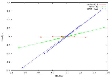
Figure 1: $\langle\tau_{n}\rangle$ in the complex plane for $x_{min}=-20.5$ (red), $-20$ (green), and $-19.5$ (blue). All for $L=20$, $N=6$, $\alpha^{\prime}=1$, $V=-\sqrt{\frac{25}{6\alpha^{\prime}}}$. In each case $\langle\tau_{1}\rangle$ is the point furthest to the left.

Since the action is space-dependent, the meaning of the infinite-volume limit is unclear. It is straightforward to decrease $x_{min}$, since the cubic term becomes exponentially small at small $x$. However, it is not clear if the limit $x_{max}\rightarrow\infty$ is well-defined, since the cubic term continues to get stronger in this direction. Indeed, we find that the imaginary parts of the $\tau_{n}$ continue to increase rapidly when we increase $x_{max}$.

3.1 Continuum limit

In momentum space, the continuum limit is approached by increasing the number of modes $N$. We can only increase $N$ up to a maximum value of $L/\pi\sqrt{\alpha^{\prime}}$ since we require $l<1$. In this range we find that the instability becomes stronger as $N$ is increased, presumably because the number of unstable cubic terms increases rapidly with $N$. We show an example in Fig. 2, where the maximum level increases from 0.05 (where $N=1$) to 0.95 ($N=6$). To approach closer to the continuum limit, we will have to include more fields at higher $l_{0}$-levels. Calculations at level-1 are in progress.

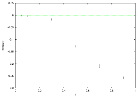
Figure 2: $Im\langle\tau_{1}\rangle$ as a function of level $l$, for $x_{min}=-20$, $L=20$, $\alpha^{\prime}=1$, $V=-\sqrt{\frac{25}{6\alpha^{\prime}}}$.

3.2 Dilaton

Finally, we have considered what happens when we vary the dilaton $V$. In the full string field theory we require $V=-\sqrt{\frac{25}{6\alpha^{\prime}}}$. We might expect that varying $V$ away from this value would increase the instability. However, this is not the case, at least for the level-0 theory. Increasing $V$ above $-\sqrt{\frac{24}{6\alpha^{\prime}}}$ changes the sign of $m_{0}^{2}$, making the theory tachyonic and hence more unstable; on the other hand decreasing $V$ makes $m_{0}^{2}$ larger and the cubic terms smaller and hence decreases the instability. Our results when we vary $V$ are consistent with this picture. However, it should be noted that decreasing $V$ does not remove the instability entirely, and it will always become strong at some sufficiently large value of $x$.

4 Conclusions

We have implemented a Monte Carlo simulation of the 1-d linear dilation truncated to zero $l_{0}$-level. We observe non-trivial quantum effects: the classical solution to the equations of motion is $\tau_{n}=0$, but we observe non-zero $\tau_{n}$. We also find that as expected, the theory is unstable at large $x$, as shown by the large imaginary parts the expectation values of the field develop.

There are several possible explanations for our result. Firstly, it may be that the instability is a real feature of the full, non-truncated theory. This should not be the case for the theory at hand. Another possibility is that the instability is just an artifact of the level-truncation. In this scenario the higher-level fields, which we have not included, would stabilise the theory. Alternatively, it might also be the case that level-truncation is not a consistent regularization of the quantum theory. Finally it is also possible that the instability represents some fundamental problem with open string field theory as a method for quantising string theory. This could be attributed, e.g., to the lack of control over closed string degrees of freedom or to the somewhat singular nature of the star product.

Calculations including level-1 fields are underway. At this level it is not obvious how to deal with the gauge and ghosts degrees of freedom, and there are several possible choices. It will be interesting to see how these compare. A practical issue is that Grassmann-odd fields will appear and will have to be dealt with.

Looking further ahead, it would be interesting to increase the number of dimensions. Ultimately the target would be to work in ten dimensions and to include fermionic degrees of freedom, with the aim of reaching a full quantum, non-perturbative definition of superstring theory.

References

- [1] E. D’Hoker and D. Phong, Lectures on two-loop superstrings, hep-th/0211111.
- [2] S. Grushevsky, Superstring scattering amplitudes in higher genus, arXiv:0803.3469 [hep-th].
- [3] P. Dunin-Barkowski, A. Morozov, and A. Sleptsov, Lattice theta constants vs Riemann theta constants and NSR superstring measures, arXiv:0908.2113 [hep-th].
- [4] E. Fuchs and M. Kroyter, Analytical solutions of open string field theory, arXiv:0807.4722 [hep-th].
- [5] A. Sen, Universality of the tachyon potential, hep-th/9911116.
- [6] N. Berkovits, Y. Okawa and B. Zwiebach, WZW-like action for heterotic string field theory, hep-th/0409018.
- [7] I. Arefeva, P. Medvedev and A. Zubarev, New representation for string field solves the consistency problem for open superstring field theory, Nucl. Phys., B341, 464 (1990).
- [8] C. Preitschopf, C. Thorn and S. Yost, Superstring field theory, Nucl. Phys., B337, 363 (1990)
- [9] N. Berkovits, Super-Poincaré invariant superstring field theory, hep-th/9503099.
- [10] M. Kroyter, Superstring field theory in the democratic picture, arXiv:0911.2962 [hep-th].
- [11] D. Friedan, E. Martinec and S. Shenker, Conformal invariance, supersymmetry and string theory, Nucl. Phys. B271, 93 (1986).
- [12] B. Zwiebach, Closed string field theory: Quantum action and the B-V master equation, hep-th/9206084.
- [13] E. Witten, Noncommutative geometry and string field theory, Nucl. Phys. B268, 253 (1986).
- [14] A. Sen, Descent relations among bosonic D-branes, hep-th/9902105.
- [15] A. Sen, Tachyon condensation in string field theory, hep-th/9912249.
- [16] M. Schnabl, Analytic solution for tachyon condensation in open string field theory, hep-th/0511286.
- [17] H. Yang and B. Zwiebach, Rolling closed string tachyons and the big crunch, hep-th/0506076.
- [18] H. Yang and B. Zwiebach, A closed string tachyon vacuum?, hep-th/0506077.
- [19] N. Moeller and H. Yang, The nonperturbative closed string tachyon vacuum to high level, hep-th/0609208.
- [20] A. A. Belavin, A. M. Polyakov and A. B. Zamolodchikov, Infinite conformal symmetry in two-dimensional quantum field theory, Nucl. Phys. B241, 333 (1984).
- [21] P. Ginsparg and G. Moore, Lectures on 2D gravity and 2D string theory, hep-th/9304011.
- [22] V. A. Kostelecky and S. Samuel, On a nonperturbative vacuum for the open bosonic string, Nucl. Phys. B336, 263 (1990).
- [23] V. A. Kostelecky and S. Samuel, The static tachyon potential in the open bosonic string, Phys. Lett. B207, 169 (1988).
- [24] D. Gaiotto and L. Rastelli, Experimental string field theory, hep-th/0211012.
- [25] E. Witten, Analytic continuation of Chern-Simons theory, arXiv:1001.2933 [hep-th].