On leave from ] Institute of Physics, Slovak Academy of Sciences, Bratislava, Slovakia

Strong-Coupling Theory of Counter-ions at Charged Plates

Abstract

We present an analytical approach to the strong coupling regime of similarly and highly charged plates in the presence of counter-ions. The procedure is physically transparent and based on an exact expansion around the ground state formed by the two-dimensional Wigner crystal of counter-ions. The one plate problem is worked out, together with the two plates situation. Unlike previous approaches, the expansion is free of divergences, and is shown to be in excellent agreement with available data of Monte-Carlo simulations under strong Coulombic couplings. The present results shed light on the like-charge attraction regime.

The behaviour of charged particles in the vicinity of charged interfaces is a central yet elusive problem in the equilibrium statistical mechanics of Coulomb fluids, including colloidal science. A landmark in the field was the realization in the 1980s that similarly charged surfaces may attract each other under strong enough Coulombic couplings, which can be realized in practice increasing the valency of the counter-ions involved Guldbrand84 ; Kjellander84 ; Kekicheff93 . Notorious illustrations of this like-charge attraction are the formation of DNA condensates Bloomfield96 or aggregates of colloidal particles Linse00 .

The weak-coupling limit is described by the Poisson-Boltzmann mean-field approach Andelman06 and by its systematic improvements via the loop expansion Attard88 ; Podgornik90 ; Netz00 . A remarkable achievement of the last decade has been accomplished in the opposite strong-coupling (SC) limit, pioneered by Rouzina and Bloomfield Rouzina96 , substantiated by Shklovskii, Levin and collaborators Shklovskii ; Levin02 , and formalized by Netz et al Moreira00 ; Netz01 ; Boroudjerdi05 . An essential ingredient is that the layer of counter-ions close to a charged wall becomes two-dimensional, and in the field-theoretical method put forward in Moreira00 ; Netz01 , the leading behaviour stems from a single-particle theory, which produces more compact profiles than within mean-field theory Messina09 . Next correction orders correspond to a virial/fugacity expansion in inverse powers of the coupling constant $\Xi$, see the definition (2) below. The method requires a renormalization of infrared divergences via the electroneutrality condition. A comparison with the Monte-Carlo (MC) simulations Moreira01 indicates the adequacy of the leading single-particle theory in the asymptotic SC limit, while capturing the first correction resisted the analysis.

The establishment of an (approximative) interpolation between the Poisson-Boltzmann and SC regimes, based on the idea of a “correlation hole”, was the subject of a series of works Nordholm84 ; Chen06 ; Santangelo06 ; Hatlo10 . The specification of the correlation hole was done empirically in Refs. Chen06 ; Santangelo06 and self-consistently, as an optimization condition for the grand partition function, in Hatlo10 . A relevant observation in Hatlo10 , corroborated by a comparison with the MC simulations, was that the first correction in the SC expansion is proportional to $1/\sqrt{\Xi}$, and not to $1/\Xi$ as suggested by the original SC theory.

The aim of this Letter is to revisit the SC limit and establish an exact expansion which, in light of the previous discussion, has yet to be formulated. The leading term of counter-ion density profiles coincides with the single-particle picture of the SC theory. Our expansion is free of infrared divergences and entails a correction in $1/\sqrt{\Xi}$ to the leading behaviour. Our analytical results are shown to be in excellent agreement with available MC data without adjustable parameters. The procedure is significantly simpler than previous works, and appears versatile. It will in particular be shown to yield new exact results in the like charge attraction regime.

Here, we study a classical system of (equally charged) counter-ions in the vicinity of one or two planar walls bearing a uniform surface charge density, $\sigma e$ ($e$ is the elementary charge and $\sigma>0$), the system as a whole being electro-neutral. The system, at thermal equilibrium at the inverse temperature $\beta=1/(k_{\rm B}T)$, is immersed in a solution of dielectric constant $\epsilon$ containing $q$-valent counter-ions, each thus having charge $-qe$. For simplicity, no image forces are present. Let us describe briefly the original SC theory Moreira00 ; Netz01 for the case of a single wall localized in the $z=0$ plane. The counter-ions are confined to the half-space $z\geq 0$. The relevant length scales in Gaussian units are: The Bjerrum length $\ell_{\rm B}=\beta e^{2}/\epsilon$, i.e. the distance at which two unit charges interact with thermal energy $k_{\rm B}T$, and the Gouy-Chapman length $\mu=1/(2\pi q\ell_{\rm B}\sigma)$, i.e. the distance from the charged wall at which an isolated counter-ion has potential energy equal to thermal energy. All lengths $r$ will be expressed in units of $\mu$, $\tilde{r}=r/\mu$. The counter-ion density profile $\rho(z)$, which only depends on the distance from the wall $z$, will be considered in the rescaled form

$$\tilde{\rho}(\tilde{z})=\frac{\rho(\tilde{z})}{2\pi\ell_{\rm B}\sigma^{2}},$$ (1)

so that the electro-neutrality condition $q\int_{0}^{\infty}dz\rho(z)=\sigma$ simply reads $\int_{0}^{\infty}d\tilde{z}\tilde{\rho}(\tilde{z})=1.$ The coupling parameter quantifying the strength of electrostatic correlations is

$$\Xi=2\pi q^{3}\ell_{\rm B}^{2}\sigma$$ (2)

and is large in the SC regime. According to the SC theory Moreira00 ; Netz01 , the profile of the counter-ion density can be formally expanded as

$$\tilde{\rho}(\tilde{z})=\tilde{\rho}_{0}(\tilde{z})+\frac{1}{\Xi}\tilde{\rho}_{1}(\tilde{z})+{\cal O}(\Xi^{-2}),$$ (3)

where

$$\tilde{\rho}_{0}(\tilde{z})={\rm e}^{-\tilde{z}},\quad\tilde{\rho}_{1}(\tilde{z})={\rm e}^{-\tilde{z}}\left(\frac{\tilde{z}^{2}}{2}-\tilde{z}\right).$$ (4)

The leading term $\tilde{\rho}_{0}(\tilde{z})$ comes from the single-particle picture of counter-ions in the linear surface-charge potential. The MC simulations Moreira01 indicate that the first correction $\tilde{\rho}_{1}(\tilde{z})$ has the expected functional form for $\Xi>10$, however, the value of the prefactor is incorrect. To be more particular, let us subtract the leading SC profile in (3) and express the first correction as

$$\tilde{\rho}_{1}(\tilde{z})=\theta\left[\tilde{\rho}(\tilde{z})-\tilde{\rho}_{0}(\tilde{z})\right],$$ (5)

$\tilde{\rho}(\tilde{z})$ being the density profile obtained from the MC simulations. The factor $\theta$ can be treated as a fitting parameter which, in the original SC theory, should be equal to $\Xi$ plus next-to-leading corrections. The numerical dependence of $\theta$ on $\Xi$ is pictured in the inset of Fig. 1. We see that $\theta$ (symbols) is much smaller than $\Xi$ (dashed line).

Our approach is based on the fact that in the asymptotic strong-coupling limit $\Xi\to\infty$, the counter-ions collapse on the charged surface, creating a 2D hexagonal (equilateral triangular) Wigner crystal Levin02 where every ion has 6 nearest neighbors forming an hexagon. Let us denote by ${\bf R}_{i}=(X_{i},Y_{i})$ the position vectors of the vertices on this hexagonal lattice. Since there are just two triangles per particle, the lattice spacing $a$ of the globally electro-neutral structure is given by $q/\sigma=\sqrt{3}a^{2}/2.$ Note that the strong-coupling limit coincides with the regime in which the distance $a$ between the nearest-neighbor counter-ions is much larger than the distance $\mu$ between the counter-ions and the charged surface Rouzina96 , $\tilde{a}\equiv a/\mu\propto\sqrt{\Xi}\gg 1.$ In the asymptotic limit $\Xi\to\infty$, each vertex ${\bf R}_{i}$ is occupied by a counter-ion $i$ $(i=1,\ldots,N;N\to\infty)$. The ground-state energy of the counter-ion system together with the homogeneous background charge is $E_{0}$. For $\Xi$ large but not infinite, the fluctuations of ions around their lattice positions start to play a role.

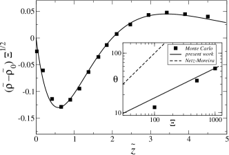
Figure 1: Comparison between the analytical first correction to the strong coupling profile (solid curve) and the Monte Carlo results of Ref. Moreira01 at $\Xi=10^{3}$, for a single charged wall. The inset compares our prediction for the rescaling factor $\theta$ (solid curve given by Eq. (12)) to its Monte Carlo value reported in Moreira01 and to the original prediction $\theta=\Xi$ (dashed line).

Let us first shift one of the particles, say $i=1$, from its lattice position ${\bf R}_{1}$ by a small vector $\delta{\bf R}_{1}=(x,y,z)$ ($\delta R_{1}\equiv|\delta{\bf R}_{1}|\ll a$) and look for the corresponding change in the total energy $\delta E=E-E_{0}\geq 0$. The first contribution to $\delta E$ comes from the interaction of the shifted counter-ion with the potential induced by the homogeneous surface charge density: $\delta E^{(1)}=2\pi qe^{2}\sigma z/\epsilon.$ The second contribution to $\delta E$ comes from the interaction of the particle with all other particles on the 2D hexagonal lattice. This contribution can be expanded as an infinite series in $x$, $y$ and $z$; for our purposes, it is sufficient to consider this expansion up to harmonic terms, which, in the $z$-direction, read

$$\epsilon\delta E^{(2)}_{z}=\sum_{i\neq 1}\left[\frac{(qe)^{2}}{\sqrt{R_{i}^{2}+z^{2}}}-\frac{(qe)^{2}}{R_{i}}\right]\sim-\frac{(qe)^{2}}{2a^{3}}Sz^{2}.$$ (6)

Here, the dimensionless quantity $S=\sum_{i\neq 1}(R_{i}/a)^{-3}$ can be expressed from the general theory of lattice sums Zucker74 ; Zucker75

$$S = \sum_{m,n=-\infty\atop(m,n)\neq(0,0)}^{\infty}\frac{1}{(m^{2}+mn+n^{2})^{3/2}}$$ (7)

$$= \frac{2}{\sqrt{3}}\zeta\left(\frac{3}{2}\right)\left[\zeta\left(\frac{3}{2},\frac{1}{3}\right)-\zeta\left(\frac{3}{2},\frac{2}{3}\right)\right],$$

where $\zeta(z,q)=\sum_{n=0}^{\infty}1/(q+n)^{z}$ is the generalized Riemann zeta function Gradshteyn and $\zeta(z)\equiv\zeta(z,1)$. Explicitly, $S=11.034\ldots$. A shift of the particle simultaneously along all directions does not induce “mixed” harmonic terms of type $xz$ or $yz$. The harmonic term in the $(x,y)$-plane can be computed, and in dimensionless form, we have

$$-\beta\delta E\sim-\tilde{z}+\frac{3^{3/4}}{(4\pi)^{3/2}}\frac{S}{\sqrt{\Xi}}\left[\frac{\tilde{z}^{2}}{2}-\frac{1}{4}\left(\tilde{x}^{2}+\tilde{y}^{2}\right)\right].$$ (8)

This formula reveals a relationship between the order of the expansion of $-\beta\delta E$ in the dimensionless lengths $\tilde{x},\tilde{y},\tilde{z}$ and the SC expansion in $1/\sqrt{\Xi}$. The linear term $-\tilde{z}$, which is the only one which does not vanish in the limit $\Xi\to\infty$, is the leading term. It corresponds to the single-particle picture, in close analogy with the previous SC theory. The harmonic terms turn out to be of the SC order $\beta(qe)^{2}\mu^{2}/a^{3}\propto 1/\sqrt{\Xi}$ and likewise, terms of the $p$th order in the variables $\tilde{x},\tilde{y},\tilde{z}$ are of the SC order $\beta(qe)^{2}\mu^{p}/a^{p+1}\propto 1/\Xi^{(p-1)/2}.$ This scheme constitutes a systematic basis for SC expansions.

The generalization of the above formalism to all particles is straightforward. We shift every particle $i=1,2,\ldots,N$ from its lattice position ${\bf R}_{i}$ by a small vector $\delta{\bf R}_{i}=(x_{i},y_{i},z_{i})$. In what follows however, we shall be interested in the counter-ion density profile which only depends on the $\tilde{z}$ coordinate. Thus, when expanding in statistical averages the Gibbs weight $\exp(-\beta\delta E)$ in powers of $1/\sqrt{\Xi}$, we can restrict ourselves to the $z$-harmonic part. The corresponding change in the total energy $\delta E$ is given by a counterpart of (8),

$$-\beta\delta E\sim-\sum_{i}\tilde{z}_{i}+\frac{3^{3/4}}{16\pi^{3/2}}\frac{1}{\sqrt{\Xi}}\sum_{i<j}\frac{(\tilde{z}_{i}-\tilde{z}_{j})^{2}}{(|{\bf R}_{i}-{\bf R}_{j}|/a)^{3}}.$$ (9)

The next simplification comes from the fact that particles are identical, exposed to the same potential induced by the surface charge, so that a summation over particle coordinates can be represented by just one auxiliary coordinate. For the density particle profile, defined by $\rho({\bf r})=\langle\sum_{i=1}^{N}\delta({\bf r}-{\bf r}_{i})\rangle=N\langle\delta({\bf r}-{\bf r}_{1})\rangle$, we get explicitly

$$\tilde{\rho}(\tilde{z})=C{\rm e}^{-\tilde{z}}\int_{0}^{\infty}d\tilde{z}^{\prime}{\rm e}^{-\tilde{z}^{\prime}}\Bigg{[}1+\frac{3^{3/4}S}{16\,\pi^{3/2}}\frac{(\tilde{z}-\tilde{z}^{\prime})^{2}}{\sqrt{\Xi}}\Bigg{]}+{\cal O}(\frac{1}{\Xi}),$$ (10)

where $C$ is determined by the normalization condition $\int\tilde{\rho}=1$. Simple algebra gives

$$\tilde{\rho}(\tilde{z}) = {\rm e}^{-\tilde{z}}+\frac{3^{3/4}}{(4\pi)^{3/2}}\frac{S}{\sqrt{\Xi}}{\rm e}^{-\tilde{z}}\left(\frac{\tilde{z}^{2}}{2}-\tilde{z}\right)+{\cal O}(\Xi^{-1}).$$

Comparing this result with the previous one (3), (4) obtained in the original SC theory Moreira00 ; Netz01 , we see that the leading terms coincide, while the first corrections have the same functional dependence in space but different prefactors. The result (LABEL:19) can be re-expressed in terms of the $\theta$-factor, introduced in the relation (5), as follows

$$\theta=\frac{(4\pi)^{3/2}}{3^{3/4}}\frac{1}{S}\sqrt{\Xi}=1.771\ldots\sqrt{\Xi}.$$ (12)

This formula, in excellent agreement with MC data, differs substantially from the previous SC estimate $\theta=\Xi$, see Fig. 1.

The method can be readily applied to the case of two parallel walls, each having the same charge density $\sigma e$, located at distance $d$ from one another. The electric field between the walls is equal to 0 now. At $T=0$, the classical system is defined by the dimensionless separation $\eta=d\sqrt{\sigma/q}=\tilde{d}/\sqrt{2\pi\Xi}$. A complication comes from the fact that counter-ions form, on the opposite surfaces, a bilayer Wigner crystal, the structure of which depends on $\eta$ Goldoni96 ; Messina03 ; Lobaskin07 . Five different structures are energetically favored for various regions of $\eta$. At the smallest separations when $\eta\to 0$, the single hexagonal lattice (structure I, see Fig. 2-left), with rows distributed consecutively between the two surfaces, is formed. At large separations $\eta>0.732$, the energetically favored geometry is composed of two staggered hexagonal lattices (structure V), one for each plate. We shall document our SC approach on structure I, relevant to obtain the large $\Xi$ behaviour. Due to global neutrality, the lattice spacing $b$ of the single (bilayer) hexagonal structure is given by $q/(2\sigma)=\sqrt{3}b^{2}/2.$ The SC regime is identified with the condition $d\ll b$, or equivalently $\Xi\gg\tilde{d}^{2}$.

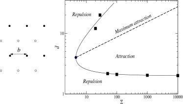
Figure 2: Left: Structure I of counter-ions on two parallel charged plates (see text). Right: Phase diagram following from the equation of state (17): the solid curve shows the points where $P=0$. The filled squares are those MC results from Ref Moreira01 with $\Xi>20$, while the dashed line is for the points where $\partial\tilde{P}/\partial\tilde{d}=0$, which defines $\tilde{d}_{\text{m}ax}$.

The two walls are located at positions $z=0$ and $z=d$. The position vector ${\bf R}_{i}$ of the particle localized on the shared hexagonal Wigner lattice will be denoted as ${\bf R}^{(0)}_{i}$ if it belongs to the wall at $z=0$ (say filled symbols of the left panel of Fig. 2) and as ${\bf R}^{(d)}_{i}$ if it belongs to the wall at $z=d$ (open symbols in Fig. 2). Let us shift the particle $i=1$ localized on the $z=0$ wall by a small vector $\delta{\bf R}_{1}^{(0)}=(x,y,z)$ and look for the energy change $\delta E$ from the ground state. Since the potential induced by the surface charge on the walls is constant between the walls, the corresponding $\delta E^{(1)}=0$. The harmonic term in the $z$-direction reads

$$\epsilon\delta E_{z}^{(2)}=\frac{(qe)^{2}}{2b^{3}}\left[-\sum_{i\neq 1}\frac{z^{2}}{(R_{i}^{(0)}/b)^{3}}+\sum_{i}\frac{d^{2}-(d-z)^{2}}{(R_{i}^{(d)}/b)^{3}}\right].$$ (13)

Using the exact values of the partial hexagonal sums Zucker75 $\sum_{i\neq 1}\left[b/R_{i}^{(0)}\right]^{3}=5S/12$, $\sum_{i}\left[b/R_{i}^{(d)}\right]^{3}=7S/12$, $\delta E_{z}^{(2)}$ turns out to be positive, as it should. The harmonic term in the $(x,y)$-plane can again be computed but proves immaterial for the sake of our purposes. When all particles are shifted from their lattice positions $\{{\bf R}_{i}\}$ by $\{\delta{\bf R}_{i}=(x_{i},y_{i},z_{i})\}$, the total energy change is given, as far as the $z$-dependent contribution is concerned, by

$$-\beta\delta E \sim -\frac{3^{3/4}}{(4\pi)^{3/2}}\frac{\sqrt{2}}{\sqrt{\Xi}}\frac{1}{2}\sum_{i,j}\frac{\tilde{d}^{2}}{(|{\bf R}_{i}^{(0)}-{\bf R}_{j}^{(d)}|/b)^{3}}$$ (14)

$$+\frac{3^{3/4}}{(4\pi)^{3/2}}\frac{\sqrt{2}}{\sqrt{\Xi}}\frac{1}{2}\sum_{i<j}\frac{(\tilde{z}_{i}-\tilde{z}_{j})^{2}}{(|{\bf R}_{i}-{\bf R}_{j}|/b)^{3}}.$$

Expanding $\exp(-\beta\delta E)$ in $1/\sqrt{\Xi}$ and enforcing electro-neutrality, the density profile $\tilde{\rho}(\tilde{z})$ is obtained in the form

$$\tilde{\rho}(\tilde{z})=\frac{2}{\tilde{d}}+\frac{1}{\theta}\frac{2}{\tilde{d}}\left[\left(\tilde{z}-\frac{\tilde{d}}{2}\right)^{2}-\frac{\tilde{d}^{2}}{12}\right]+{\cal O}(\Xi^{-1})~{}$$ (15)

$$\hbox{where }\quad\theta=\frac{(4\pi)^{3/2}}{3^{3/4}}\frac{1}{S}\frac{\sqrt{\Xi}}{\sqrt{2}}=1.252\ldots\sqrt{\Xi}.$$ (16)

This $\theta$ differs from the single-plate one (12) by the factor $1/\sqrt{2}$ due to the different hexagonal lattice spacings $a$ and $b$. The functional form of (15) coincides with that of Moreira and Netz Moreira00 ; Netz01 . For (not yet asymptotic) $\Xi=100$, the previous SC result $\theta=\Xi$ is far away from the MC estimate $\theta\simeq 11.2$ Moreira01 , while our formula (16) gives $\theta\simeq 12.5$.

Applying the contact-value theorem to the density profile (15), the pressure $P$ between the plates is given by

$$\tilde{P}\,=\,\frac{P}{2\pi\ell_{B}\sigma^{2}}\,=\,-1+\frac{2}{\tilde{d}}+\frac{\tilde{d}}{3\theta}+{\cal O}\left(\frac{\tilde{d}^{2}}{\Xi}\right).$$ (17)

An analogous result was obtained within the approximate approach of Ref. Hatlo10 , with the underestimated ratio $\theta/\sqrt{\Xi}=3\sqrt{3}/2=0.866\ldots$. We recall that our estimate of $\theta$ is valid only in the structure I region $0\leq\eta<0.006$; increasing $\eta$, other energetically favored bilayer Wigner structures have to be considered as a starting point. Eq. (17) provides insight into the like charge attraction phenomenon. The attractive ($P<0$) and repulsive ($P>0$) regimes are shown in Fig. 2 (right panel). Although our results hold for $\tilde{d}\ll\Xi^{1/2}$ and for large $\Xi$, the shape of the phases boundaries where $P=0$ (solid curve) shows striking similarity with its counterpart obtained numerically Moreira01 ; Chen06 (we note for instance that the terminal point shown by the filled circle in Fig 2 is located at $\tilde{d}=4$, a value close to that which can be extracted from Moreira01 ; Chen06 ). While the upper branch of the attraction/repulsion boundary is such that $\tilde{d}/\sqrt{\Xi}$ is of order unity and hence lies at the limit of validity of our expansion, we predict the maximum attraction to be obtained for $\tilde{d}_{\text{max}}=\sqrt{6\theta}\propto\Xi^{1/4}$, as follows from enforcing $\partial\tilde{P}/\partial\tilde{d}=0$. Since $\tilde{d}_{\text{max}}/\sqrt{\Xi}\propto\Xi^{-1/4}\to 0$, we can consider the latter prediction, shown by the dashed line in Fig. 2, as asymptotically exact; we note that it is fully corroborated by the scaling laws reported in Chen06 .

In conclusion, the present exact approach to the strong coupling regime shows that while the leading order results at large $\Xi$ (for one or two plates) can be obtained by a single counter-ion theory, the next terms actually reflect the complete ground state structure ($N$ counter-ion property). This explains the failure of virial-like expansions. We have shown how such shortcomings can be circumvented within a physically transparent procedure, and obtained analytical results in remarkable agreement with Monte Carlo data. In practice, for a highly charged interface in water at room $T$, one has $\sigma\ell_{\rm{B}}^{2}\simeq 1$, so that $\Xi$ takes values close to 50, 170 and 400 for respectively di-, tri-, and tetra-valent counter-ions, as often found in biology (spermine). Although asymptotic, our predictions turn out to be reliable for such couplings. A generalization of the approach to dielectric inhomogeneities Jho08 , systems with salt or asymmetric Kanduc10 , and curved surfaces Santos09 , offer interesting problems for more detailed studies in the future. The formulation is also convenient for a quantum-mechanical generalization.

- (1) L. Guldbrand, B. Jönson, H. Wennerström and P. Linse, J. Chem. Phys. 80, 2221 (1984).
- (2) R. Kjellander and S. Marčelja, Chem. Phys. Lett. 112, 49 (1984).
- (3) P. Kékicheff, S. Marčelja, T.J. Senden and V.E. Shubin, J. Chem. Phys. 99, 6098 (1993).
- (4) V.A. Bloomfield, Curr. Opin. Struct. Biol. 6, 334 (1996).
- (5) P. Linse and V. Lobaskin, Phys. Rev. Lett. 83, 4208 (1999).
- (6) D. Andelman, in Soft Condensed Matter Physics in Molecular and Cell Biology, edited by W. C. K. Poon and D. Andelman (Taylor & Francis, New York, 2006).
- (7) P. Attard, D. J. Mitchell, and B. W. Ninham, J. Chem. Phys. 88, 4987 (1988); ibid 89, 4358 (1988).
- (8) R. Podgornik, J. Phys. A 23, 275 (1990).
- (9) R. R. Netz, H. Orland, Eur. Phys. J. E 1, 203 (2000).
- (10) I. Rouzina and V.A. Bloomfield, J. Phys. Chem. 100, 9977 (1996).
- (11) A.Y. Grosberg, T.T. Nguyen and B.I. Shklovskii, Rev. Mod. Phys. 74, 329 (2002).
- (12) Y. Levin, Rep. Prog. Phys. 65, 1577 (2002).
- (13) A. G. Moreira and R. R. Netz, Europhys. Lett. 52, 705 (2000).
- (14) R. R. Netz, Eur. Phys. J. E 5, 557 (2001).
- (15) H. Boroudjerdi et al., Phys. Rep. 416, 129 (2005).
- (16) R. Messina, J. Phys.: Condens. Matter 21 113102 (2009).
- (17) A. G. Moreira and R. R. Netz, Phys. Rev. Lett. 87, 078301 (2001); Eur. Phys. J. E 8, 33 (2002).
- (18) S. Nordholm, Chem. Phys. Lett. 105, 302 (1984).
- (19) Y. G. Chen and J. D. Weeks, Proc. Natl. Acad. Sci. U.S.A. 103, 7560 (2006); J.M. Rodgers, C. Kaur, Y.G. Chen and J.D. Weeks, Phys. Rev. Lett. 97, 097801 (2006).
- (20) C. D. Santangelo, Phys. Rev. E 73, 041512 (2006).
- (21) M. Hatlo and L. Lue, Europhys. Lett. 89, 25002 (2010).
- (22) I. J. Zucker, J. Math. Phys. 15, 187 (1974).
- (23) I. J. Zucker and M. M. Robertson, J. Phys. A 8, 874 (1975).
- (24) I. S. Gradshteyn and I. M. Ryzhik, Table of Integrals, Series and Products, 5th edn. (Acad. Press, London, 1994).
- (25) G. Goldoni and F. M. Peeters, Phys. Rev. B 53, 4591 (1996).
- (26) R. Messina and H. Löwen, Phys. Rev. Lett. 91, 146101 (2003); E.C. Oǧuz, R. Messina and H. Löwen, Europhys. Lett. 86, 28002 (2009).
- (27) V. Lobaskin and R. R. Netz, Europhys. Lett. 77, 38003 (2007).
- (28) Y.S. Jho, M. Kanduc, A. Naji, R. Podgornik, M.W. Kim and P.A. Pincus, Phys. Rev. Lett. 101, 188101 (2008).
- (29) M. Kanduc et al, J. Chem. Phys. 132, 124701 (2010); Phys. Rev. E 78, 061105 (2008).
- (30) A. P. dos Santos, A. Diehl, and Y. Levin, J. Chem. Phys. 130, 124110 (2009).