Effects of a Cut, Lorentz-Boosted sky on the Angular Power Spectrum

Abstract

The largest fluctuation in the observed CMB temperature field is the dipole, its origin being usually attributed to the Doppler Effect – the Earth’s velocity with respect to the CMB rest frame. The lowest order boost correction to temperature multipolar coefficients appears only as a second order correction in the temperature power spectrum, $C_{\ell}$. Since $v/c\sim 10^{-3}$, this effect can be safely ignored when estimating cosmological parameters Challinor:2002zh ; Kamionkowski:2002nd ; Kosowsky:2010jm ; Amendola:2010ty . However, by cutting our galaxy from the CMB sky we induce large-angle anisotropies in the data. In this case, the corrections to the cut-sky $C_{\ell}$s show up already at first order in the boost parameter. In this paper we investigate this issue and argue that this effect might turn out to be important when reconstructing the power spectrum from the cut-sky data.

I Introduction

In the last decade, cosmology has become a precision science, driven largely by measurements of the fluctuations in the Cosmic Microwave Background (CMB) temperature. These fluctuations – nearly $10^{5}$ times smaller than the average temperature of the universe – are the primary window onto most cosmological parameters Larson:2010gs . Because the fluctuations are so small, one must know the contributions to the measured temperature field from foregrounds and other contaminants. A great deal of effort has been put in to characterizing foreground signals from dust, synchrotron, and free-free emission Gold:2010fm . Even so, when inferring cosmological parameters significant fractions of the sky are usually omitted (“cut”) from full-sky maps in order to minimize effects from non-primordial sources Bennett:2003ca .

Surprisingly, one particular known systematic effect – the distortion of the CMB radiation due to our motion relative to the preferred cosmological frame – has been given comparatively little attention Challinor:2002zh ; Kamionkowski:2002nd ; Kosowsky:2010jm ; Amendola:2010ty . It has become accepted practice to simply remove the dipole from a sky map before calculating the power spectrum Hinshaw:2003ex . This is based on the belief that the effect on $C_{\ell}$, the $\ell$th element of the angular power spectrum of the temperature anisotropy, (the central quantity in cosmological parameter estimation in the context of the canonical Lambda Cold Dark Matter model, aka $\Lambda$CDM) is proportional to $\beta^{\ell}$, where $\beta\sim 10^{-3}$ is our speed relative to the cosmological frame (as determined by the magnitude of that CMB dipole). In this context, the dipole is indeed the only multipole for which the Doppler shift due to our motion is significant. Nevertheless, it has been shown Schwarz:2004gk that the second order (${\cal O}(\beta^{2})$) Doppler effect noticeably alters the directions of the quadrupole multipole vectors, which characterize the shape of the quadrupole, despite the fact that it contributes negligibly to $C_{2}$, the strength of the quadrupole.

Meanwhile, several groups have independently examined (to order $\beta^{2}$) the effect of Lorentz boosting the CMB, and determined that there are actually significant contributions to higher multipoles Challinor:2002zh ; Kamionkowski:2002nd ; Kosowsky:2010jm ; Amendola:2010ty . It has also separately been shown that simply masking a map induces correlations among nearby multipoles Hivon:2001jp . These two phenomena highlight a need for characterizing the effect of masking a Lorentz-boosted temperature field, since the process will undoubtedly mix higher multipoles of the true temperature field that have boost corrections.

This paper is organized as follows: in Section II we discuss the effect of boosting the multipole moments of the CMB, in Section III we derive an expression for the boosted pseudo power spectrum, in Section IV we show preliminary numerical estimates for corrections to the power spectrum and discuss their significance, as well as portions of the project that will be explored in future papers.

II The effects of boosts on the multipole moments of the angular power spectrum of the CMB

If an observer in the rest frame of the CMB (denoted $S$) measures a photon of frequency $\nu$ arriving along a line of sight $\hat{\bf{n}}$, then an observer in another frame $S^{\prime}$ that is moving with respect to the CMB at velocity $v\hat{\bf{v}}$ will measure the incoming photon to be arriving along a different line-of-sight $\hat{\bf{n}}^{\prime}$ with a different frequency $\nu^{\prime}$. (Note that we will not concern ourselves here with any ambiguities in determining S associated with the existence of inhomogeneities, in particular a cosmological dipole, on the assumption that that dipole is ${\cal O}(10^{-5})$ smaller than the effects we will uncover.) The motion of the observer in $S^{\prime}$ thus induces two effects: a Doppler shift in the photon frequency and an aberration – a shift in the direction from which the photon arrives. These two effects can be seen explicitly in the relation between $\hat{\bf{n}}$ and $\hat{\bf{n}}^{\prime}$

$$\hat{\bf{n}}^{\prime}=\left(\frac{\cos\theta+\beta}{1+\beta\cos\theta}\right)\hat{\bf{v}}+\frac{\hat{\bf{n}}-\cos\theta\hat{\bf{v}}}{\gamma(1+\beta\cos\theta)},$$ (1)

where $\beta\equiv v/c$ and $\cos\theta\equiv\hat{\bf{n}}\cdot\hat{\bf{v}}$. The change in observed frequency in $S^{\prime}$ is given by a simple Lorentz transformation

$$\nu^{\prime}=\gamma\nu(1+\beta\cos\theta)\,,$$ (2)

where $\gamma=(1-\beta^{2})^{-1/2}$ is the standard Lorentz factor. This angle $\theta$ is related to the angle $\theta^{\prime}$, measured in the frame $S^{\prime}$, via

$$\cos\theta^{\prime}={\frac{\cos\theta+\beta}{1+\beta\cos\theta}}\,.$$ (3)

Because of these two effects, we would like to boost the measured intensity, $I(\nu,\hat{\bf{n}})$ (the incident CMB power per unit area per unit frequency, per solid angle), and then relate the spherical harmonic coefficients of the intensity to the traditional temperature fluctuation coefficients. First, we will need the relation between the observed intensity in each frame gravitationbook ,

$$I^{\prime}(\nu,\hat{\bf{n}}^{\prime})=\gamma^{3}\left(1+\beta\cos\theta\right)^{3}I(\nu,\hat{\bf{n}}).$$ (4)

Expanding both sides in terms of spin-weighted spherical harmonics (${}_{s}Y_{\ell m}$) and using the fact that $d\hat{\bf{n}}^{\prime}=\gamma^{-2}\left(1+\beta\cos\theta\right)^{-2}d\hat{\bf{n}}$ McKinley2 , we get the following expression for the boosted multipole moments, $a_{\ell m}^{\prime}(\nu^{\prime})$, in terms of the rest-frame multipole moments $a_{\ell m}(\nu)$:

$$a_{\ell_{1}m_{1}}^{\prime}(\nu^{\prime})=\sum_{\ell_{2},m_{2}}\int{d\hat{\bf{n}}\gamma(1+\beta\cos\theta)a_{\ell_{2}m_{2}}(\nu)_{s}Y_{\ell_{2}m_{2}}(\hat{\bf{n}})_{s}Y_{\ell_{1}m_{1}}^{\ast}(\hat{\bf{n}}^{\prime})}.$$ (5)

We use the spin-weighted spherical harmonics to keep the expression completely general, so that the effect of the boost on the measured CMB spectrum can be explored for temperature fluctuations as well as polarization. Note that we have also implicitly chosen a frame where $\beta\bf{\hat{v}}$ is in the $\bf{\hat{z}}$ direction.

Expression (5) can be expanded as a series in $\beta$ by means of Eqs. (1) and (2). The expression to order $\beta^{2}$ can be found in the appendix. To order $\beta$ we find (consistent with Challinor:2002zh ):

$$a^{\prime}_{\ell m}(\nu^{\prime}) = \left[1-\frac{\beta sm}{\ell(\ell+1)}\left(2-\nu^{\prime}\frac{d}{d\nu^{\prime}}\right)\right]a_{\ell m}(\nu^{\prime})$$ (6)

$$-\beta{}_{s}\xi_{(\ell+1)m}\left[(\ell-1)+\nu^{\prime}\frac{d}{d\nu^{\prime}}\right]a_{(\ell+1)m}(\nu^{\prime})-\beta{}_{s}\xi_{\ell m}\left[-(\ell+2)+\nu^{\prime}\frac{d}{d\nu^{\prime}}\right]a_{(\ell-1)m}(\nu^{\prime})$$

where

$${}_{s}\xi_{\ell m}\equiv\sqrt{\frac{(\ell^{2}-m^{2})(\ell^{2}-s^{2})}{\ell^{2}(2\ell+1)(2\ell-1)}}\,.$$

Here, the multipole moments are the frequency dependent intensity coefficients. The more familiar temperature coefficients can be deduced from the coefficients above through the Stefan-Boltzmann law, which for fluctuations and a series expansion to $\mathcal{O}(\beta)$ reads:

$$\frac{\delta T(\hat{\bf{n}})}{T_{0}}=\frac{1}{4}\frac{\delta I(\hat{\bf{n}})}{I_{0}}$$ (7)

where

$$I(\hat{\bf{n}})=\int_{0}^{\infty}I(\nu,\hat{\bf{n}})d\nu$$ (8)

is the incident CMB power per unit area per solid angle and $T_{0}$ and $I_{0}$ are sky averages (monopoles). Therefore, in order to get the temperature multipole moments we integrate Eq.(6) over all frequencies (making use of the fact that the $a^{\prime}_{\ell m}(\nu^{\prime})$ are Planck distributed) and divide the result by four times the average intensity per solid angle . To first order in $\beta$ we have for the temperature $a^{\prime}_{\ell m}$ ($s=0$):

$$a^{\prime}_{\ell m}=a_{\ell m}+\beta\xi^{+}_{\ell m}a_{(\ell+1)m}+\beta\xi^{-}_{\ell m}a_{(\ell-1)m}$$ (9)

where the conversion factor from temperature to intensity was absorbed into the multipolar coefficients and

$$\xi^{+}_{\ell m}\equiv-(\ell-2)\,{}_{0}\xi_{(\ell+1)m}\,,\quad\xi^{-}_{\ell m}\equiv(\ell+3)\,{}_{0}\xi_{\ell m}\,.$$ (10)

We would now like to estimate the bias induced by the boost on the temperature power spectrum. Before getting into the details of the calculation, it is first necessary to define two quantities. Throughout this paper we will make the distinction between the theoretical power spectrum, given by

$$\langle a_{\ell m}a^{*}_{\ell^{\prime}m^{\prime}}\rangle=\delta_{\ell,\ell^{\prime}}\ \delta_{m,m^{\prime}}\ C_{\ell},$$ (11)

and the measured power spectrum (also referred to as the power spectrum estimator), given by

$$\mathcal{C}_{\ell}\equiv\frac{1}{2\ell+1}\sum_{m}\lvert a_{\ell m}\rvert^{2}.$$ (12)

To estimate this bias we need to go second order in the expansion (9) since the $C_{\ell}$s are quadratic in $a_{\ell m}$ (see the appendix for details). The key point here is that, on the assumption of statistical isotropy of the unboosted $a_{\ell m}$, the smallest $\beta$ correction to the boosted power spectrum is given by Challinor:2002zh :

$$\langle{\mathcal{C}}^{\prime}_{\ell}\rangle\approx C_{\ell}(1+4\beta^{2}+\mathcal{O}(\beta^{3}))\,.$$ (13)

Note that the main effect is a rescaling of the spectrum by an overall amplitude $1+4\beta^{2}$. Moreover, since $\beta\sim 10^{-3}$, the boosted power spectrum is essentially unbiased. We will now show that this conclusion may not be true in the case where the boosted spectrum is reconstructed from a cut-sky.

III Masking effects on the boosted angular power spectrum

When analyzing CMB temperature maps, it is common practice to mask regions of the sky that are believed to be contaminated. The region masked most often is the galaxy, where the observed temperature signal is known not to come from the surface of last scattering. In this case, we have a new expression for the measured temperature fluctuations:

$$\Delta\tilde{T}(\textbf{n})=\sum_{\ell>0}\sum_{m=-\ell}^{\ell}a_{\ell m}W(\textbf{n})Y_{\ell m}(\textbf{n}),$$ (14)

where $W(\textbf{n})$ is a window function described by the mask. One can then decompose the left hand side of Eq.(14) and solve for $\tilde{a}_{\ell m}$ in terms of $a_{\ell m}$. We then get the linear relation

$$\tilde{a}_{\ell_{1}m_{1}}=\sum_{\ell_{2},m_{2}}a_{\ell_{2}m_{2}}K_{\ell_{1}m_{1}\ell_{2}m_{2}}.$$ (15)

Here $K_{\ell_{1}m_{1}\ell_{2}m_{2}}$ is a general kernel that contains all of the information about the window function, $W(\textbf{n})=\sum_{\ell_{1}m_{1}}w_{\ell_{1}m_{1}}Y_{\ell_{1}m_{1}}(\textbf{n})$. It is given explicitly by

$$K_{\ell_{1}m_{1}\ell_{2}m_{2}}\equiv\sum_{\ell_{3},m_{3}}w_{\ell_{3}m_{3}}(-1)^{m_{2}}\left[\frac{(2\ell_{1}+1)(2\ell_{2}+1)(2\ell_{3}+1)}{4\pi}\right]^{\frac{1}{2}}$$

$$\times\left(\begin{array}[]{ccc}\ell_{1}&\ell_{2}&\ell_{3}\\ 0&0&0\end{array}\right)\left(\begin{array}[]{ccc}\ell_{1}&\ell_{2}&\ell_{3}\\ m_{1}&-m_{2}&m_{3}\end{array}\right),$$ (20)

where the $3\times 2$ matrices are the Wigner 3-j symbols. This can be used to find the pseudo power spectrum estimator:

$$\mathcal{\tilde{C}}_{\ell}=\frac{1}{2\ell+1}\sum_{m=-\ell}^{\ell}\lvert\tilde{a}_{\ell m}\rvert^{2}.$$ (21)

These $\mathcal{\tilde{C}}_{\ell}$s are not unbiased estimators for the true $C_{\ell}$s, but assuming statistical isotropy their expectation values are related by a real and symmetric mode coupling matrix,

$$\langle\tilde{\mathcal{C}}_{\ell_{1}}\rangle=\sum_{\ell_{2}}\mathcal{M}_{\ell_{1}\ell_{2}}\langle\mathcal{C}_{\ell_{2}}\rangle=\sum_{\ell_{2}}\mathcal{M}_{\ell_{1}\ell_{2}}C_{\ell_{2}},$$ (22)

where

$$\mathcal{M}_{\ell_{1}\ell_{2}}=\frac{2\ell_{2}+1}{4\pi}\sum_{\ell_{3}}(2\ell_{3}+1)\mathcal{W}_{\ell_{3}}\left(\begin{matrix}\ell_{1}&\ell_{2}&\ell_{3}\\ 0&0&0\end{matrix}\right)^{2}$$ (23)

and $\mathcal{W}_{\ell}=1/(2\ell+1)\sum_{m}|w_{\ell m}|^{2}$ is the power spectrum of the window function Hivon:2001jp .

We can therefore obtain an estimator for $C_{\ell}$ by approximately re-writing the relation with $\langle\mathcal{\tilde{C}}_{\ell}\rangle$ replaced by its observed value on the sky $\mathcal{\tilde{C}}_{\ell_{1}}^{obs}\simeq\sum_{\ell_{2}}\mathcal{M}_{\ell_{1}\ell_{2}}\mathcal{C}_{\ell_{2}}$. We approximately invert Eq.(22) to obtain the true $C_{\ell}$s from the pseudo ones. However, this prescription is complicated by Lorentz boosts. Since the masking procedure is unavoidably performed in the boosted frame, we no longer get a simple mode-coupling relation as in Eq.(22). Instead, we will now have a more general expression:

$$\langle\mathcal{\tilde{C}}_{\ell_{1}}^{\prime}\rangle = \frac{1}{2\ell_{1}+1}\sum_{m_{1}=-\ell_{1}}^{\ell_{1}}|\tilde{a}^{\prime}_{\ell_{1}m_{1}}|^{2}$$ (24)

$$= \frac{1}{2\ell_{1}+1}\sum_{m_{1}=-\ell_{1}}^{\ell_{1}}\sum_{\ell_{2}m_{2}}\sum_{\ell_{3}m_{3}}\langle a_{\ell_{2}m_{2}}^{\prime}a_{\ell_{3}m_{3}}^{\ast\prime}\rangle K_{\ell_{1}m_{1}\ell_{2}m_{2}}K_{\ell_{1}m_{1}\ell_{3}m_{3}}^{\ast},$$

where the multipolar coefficients are given by Eq.(9). Note that the kernels in this expression couple all the elements of the non-diagonal covariance matrix $\langle a_{\ell_{1}m_{1}}^{\prime}a_{\ell_{2}m_{2}}^{\ast\prime}\rangle$. As a consequence, linear $\beta$ terms which were absent in Eq.(9) will now contribute to the window function multipolar coefficients.

Going back to expression Eq.(24), note that to first order in $\beta$ there will only be coupling between $\ell_{2}$ and $\ell_{3}$ satisfying $|\ell_{2}-1|\leq\ell_{3}\leq\ell_{2}+1$. Therefore this expression can be re-written as

$$\langle\mathcal{\tilde{C}}_{\ell_{1}}^{\prime}\rangle=\frac{1}{2\ell_{1}+1}\sum_{m_{1}=-\ell_{1}}^{\ell_{1}}\sum_{\ell_{2},m_{2}}\sum_{m_{3},\ell_{3}=\ell_{2}-1}^{\ell_{2}+1}\langle a_{\ell_{2}m_{2}}^{\prime}a_{\ell_{3}m_{3}}^{\ast\prime}\rangle K_{\ell_{1}m_{1}\ell_{2}m_{2}}K_{\ell_{1}m_{1}\ell_{3}m_{3}}^{\ast}.$$ (25)

When writing out each term in the sum over $\ell_{3}$ and plugging in the expression for $a_{\ell_{2}m_{2}}^{\prime}$ (see Eq.(9)), we arrive at the following relation between the boosted pseudo-$\mathcal{C}_{\ell}$’s and the expectation values of the CMB rest frame, $C_{\ell}$’s:

$$\langle\mathcal{\tilde{C}}^{\prime}_{\ell_{1}}\rangle=\sum_{\ell_{2}}\left(\mathcal{M}_{\ell_{1}\ell_{2}}C_{\ell_{2}}+\mathcal{N}_{\ell_{1}\ell_{2}}C_{\ell_{2}}+\mathcal{P}_{\ell_{1}\ell_{2}}C_{\ell_{2}+1}+\mathcal{Q}_{\ell_{1}\ell_{2}}C_{\ell_{2}-1}\right)$$ (26)

where

$$\mathcal{N}_{\ell_{1}\ell_{2}} = \frac{\beta}{2\ell_{1}+1}\sum_{m_{1},m_{2}}K_{\ell_{1}m_{1}\ell_{2}m_{2}}\left(K_{\ell_{1}m_{1}(\ell_{2}+1)m_{2}}^{*}\xi_{(\ell_{2}+1)m}^{-}+K_{\ell_{1}m_{1}(\ell_{2}-1)m_{2}}^{*}\xi_{(\ell_{2}-1)m}^{+}\right)\,,$$ (27)

$$\mathcal{P}_{\ell_{1}\ell_{2}} = \frac{\beta}{2\ell_{1}+1}\sum_{m_{1},m_{2}}K_{\ell_{1}m_{1}\ell_{2}m_{2}}K_{\ell_{1}m_{1}(\ell_{2}+1)m_{2}}^{*}\xi_{\ell_{2}m_{2}}^{+}\,,$$ (28)

$$\mathcal{Q}_{\ell_{1}\ell_{2}} = \frac{\beta}{2\ell_{1}+1}\sum_{m_{1},m_{2}}K_{\ell_{1}m_{1}\ell_{2}m_{2}}K_{\ell_{1}m_{1}(\ell_{2}-1)m_{2}}^{*}\xi_{\ell_{2}m_{2}}^{-}\,.$$ (29)

Ignoring ”fence-post” terms and re-indexing the sum, we can re-write Eq.(30) as

$$\langle\tilde{\mathcal{C}}^{\prime}_{\ell_{1}}\rangle\approx\sum_{\ell_{2}}\left(\mathcal{M}_{\ell_{1}\ell_{2}}+\mathcal{N}_{\ell_{1}\ell_{2}}+\mathcal{P}_{\ell_{1}\ell_{2}-1}+\mathcal{Q}_{\ell_{1}\ell_{2}+1}\right)C_{\ell_{2}}$$ (30)

Clearly, the boosted pseudo power spectra in Eq.(30) are far from being unbiased estimators of the $C_{\ell}$s. If we neglect the boost effects on the $\mathcal{C}_{\ell}$s and only multiply by $\mathcal{M}^{-1}$ to solve for the values of the $C_{\ell}$s, then we will obtain an unbiased estimate since $\mathcal{N}$, $\mathcal{P}$, and $\mathcal{Q}$ are $\beta$-dependent. Furthermore, the bias in Eq.(30) produces more than just an overall multiplicative constant, since the matrices $\mathcal{M}$, $\mathcal{N}$, $\mathcal{P}$ and $\mathcal{Q}$ are not in general peaked at $\ell_{2}\approx\ell_{1}$. The correct reconstruction of the true $C_{\ell}$s depends on the careful inversion of the sum of the four matrices above. Before carrying a complete numerical analysis, we must analyze the type of couplings that the matrices $\mathcal{N}$, $\mathcal{P}$ and $\mathcal{Q}$ induce on the pseudo-power spectrum. This is the subject of the next section.

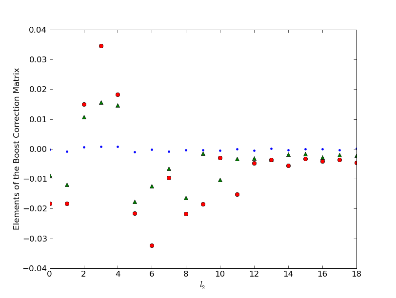
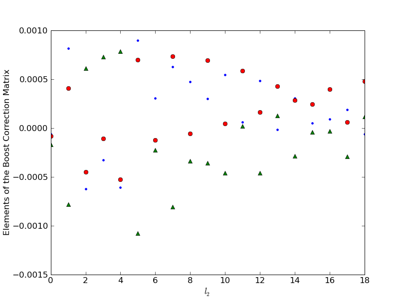
Figure 1: The top figure shows the effect of moving the mask north by 5 degrees with respect to the galactic equator. Note that there are significant changes in contribution to the correction matrix elements as the mask is moved to 76-105 degrees (blue dots), 86-115 degrees (green triangles), and 96-125 degrees (red circles). The bottom figure shows the effect of varying mask size while keeping it only 1 degree north-south asymmetric for 76-105 (green triangles), 79-100 (blue dots), and 84-95 (red circles) degree masks. Here we notice slight changes in the matrix elements when the masks decrease in size, however the effect is very small when compared to the effect of moving the mask off-center. All of these values were generated with $\ell_{1}=5$.

III.1 Example: Equatorial Strip

Before we calculate these couplings explicitly, we should mention two important points. First, in this section we will examine only the special case where both the boost and the normal to the mask are in the $z$-direction. This is of course unlikely to be correct. It is also likely to underestimate the magnitude of the effects we are examining. A thorough analysis that also includes the angle between the boost and the galactic plane as a free parameter is being carried out and will be reported on in a future work. Our point here is to note that $\beta$ corrections exist regardless of this direction, and might in turn affect the reconstruction of the true $C_{\ell}$s if the boost is not correctly accounted for. Second, given that linear corrections will induce couplings of the form $(\ell_{(1,2)},\ell_{(2,1)}\pm 1)$ and because of the restriction that $\ell_{1}+\ell_{2}+\ell_{3}$ must be even in Eq.(III), the effect uncovered is a mixed-parity one. This means that $\beta$ corrections are identically zero for masks which are even or odd functions. Real CMB masks do not possess well-defined parity, a fact which further points to the importance of the analysis being carried out here.

To illustrate the type of coupling induced by the matrices (27-29), we have carried out a numerical analysis using a north-south asymmetric equatorial strip as a mask with different widths and degrees of asymmetry. Figure 1 show some plots of these matrices for $\ell_{1}=5$ as a function of $\ell_{2}$. Noticeably, the main difference between (27-29) and the matrix (23) is that the former assume both positive and negative values, whereas the latter is a positive-definite matrix. Regarding their amplitude, we have checked that matrices $\mathcal{N}$, $\mathcal{P}$ and $\mathcal{Q}$ can be as large as 15% of matrix $\mathcal{M}$ for the range of $\ell_{2}$ shown in Fig. 1. Including the $\beta$ factor, this should amount to a correction of order $10^{-4}$ to Eq.(22). This may look smaller than the known $10^{-3}$ signal present in the off-diagonal terms of full-sky correlation matrices Challinor:2002zh ; Amendola:2010ty . However, we emphasize that here we are proposing a correction to the reconstructed true $C_{\ell}$s, and not cross-terms of the correlation matrix as discussed in Amendola:2010ty ; the former are not only less noise contaminated but also have a smaller cosmic variance.

IV Discussion and Future Work

Determining our direction and velocity with respect to the CMB rest frame is a fundamental quest for the standard cosmological model. While the main observable effects, noticeably the dipole, was already detected in the late 70’s Smoot:1977bs , higher multipolar distortions in the temperature field may yet be uncovered by future high-resolution data from the Planck satellite. In this paper we have shown that the CMB power spectrum may be systematically contaminated by this effect already at first order in the boost parameter if the boost effect is not taken into account when reconstructing full-sky data from cut-skies. We estimated this effect as a $10^{-4}$ signal in the pseudo $\mathcal{C}_{\ell}$s. Although this may seem smaller than the signal in off-diagonal full-sky CMB observables, only a careful reconstruction of full-sky data will be able to set this issue. We have also shown, using a simple strip as a mask, that the boost couples different multipoles in a way which is in sharp contrast to the couplings induced by the mask alone. Since the masking procedure is known to induce large-angle correlations, reconstructing the $\mathcal{C}_{\ell}$s correctly may have a sizable impact in tracing systematics and/or accounting for large-angle anomalies.

In a companion paper we will carry a more complete analysis of these effects, including the angle between the boost and the galactic plane as a free parameter. This angle dependence will lead to further couplings between the boost and the mask which might be used as a further estimator of the boost direction.

Since not all of the available information is contained in the $C_{\ell}$’s (due to the coupling between nearby modes of the $a_{\ell m}^{\prime}$), we will define off-diagonal estimators of the covariance matrix. Additionally, we will determine the likelihood of finding the direction of $\beta$ from our boosted covariance matrix. Both of these issues have been discussed in part by Amendola:2010ty . We will also be looking into the effect of cut skies on reconstructing polarization estimators, which can be carried out starting from expression 6 and setting $s=2$.

Appendix A Second order results

A.1 Multipolar coefficients

For completeness, we present here the expansion in the brightness multipolar coefficients to second order in the boost parameter. Similar expansions can also be found in Challinor:2002zh ; Amendola:2010ty We now want to expand Eq. 5 to $\mathcal{O}(\beta^{2})$. We begin by re-writing

$$\gamma(1+\beta\cos\theta)\simeq 1+\beta\cos\theta+\frac{1}{2}\beta^{2}$$ (31)

and $a_{\ell_{2}m_{2}}(\nu)$ using

$$a_{\ell m}(\nu)\simeq a_{\ell m}(\nu^{\prime})+\left(\beta^{2}\cos^{2}\theta-\frac{\beta^{2}}{2}-\beta\cos\theta\right)\nu^{\prime}\frac{d}{d\nu^{\prime}}a_{\ell m}(\nu^{\prime})+\left(\beta^{2}\cos^{2}\theta\right)\frac{\nu^{\prime 2}}{2}\frac{d^{2}}{d\nu^{\prime 2}}a_{\ell m}(\nu^{\prime})$$ (32)

We will also expand ${}_{s}Y_{\ell_{1}m_{1}}^{\ast}(\hat{\bf{n}}^{\prime})$ about $\hat{\bf{n}}$ to get

$${}_{s}Y_{\ell m}(\hat{\bf{n}}^{\prime})=\,_{s}Y_{\ell m}^{\ast}(\hat{\bf{n}})-\beta\sin\theta\left(1+\beta\cos\theta\right){\partial_{s}Y_{\ell m}^{\ast}(\hat{\bf{n}})\over\partial\cos\theta}\,+\frac{\beta^{2}\sin^{2}\theta}{2}{\partial^{2}\,_{s}Y_{\ell m}^{\ast}(\hat{\bf{n}})\over\partial\cos\theta^{2}}.$$ (33)

There is a general expression for writing the derivatives of a spherical harmonic in terms of other spherical harmonics (valid for $\ell\geq 1$)abramowitz+stegun :

$$\sin\theta\,{\partial_{s}Y_{\ell m}\over\partial\cos\theta}=\ell\sqrt{\frac{(\ell+1)^{2}-m^{2}}{(2\ell+1)(2\ell+3)}}\,_{s}Y_{\ell+1,m}+\frac{sm}{\ell(\ell+1)}\,_{s}Y_{\ell,m}-(\ell+1)\sqrt{{\ell^{2}-m^{2}\over(2\ell+1)(2\ell-1)}}\,_{s}Y_{\ell-1,m}$$ (34)

We also see that there will be some $\beta\cos\theta$ cross terms to deal with, which can be done using the formula

$$\cos\theta\,_{s}Y_{\ell m}=\sqrt{{(\ell+1)^{2}-m^{2}\over(2\ell+1)(2\ell+3)}}\,_{s}Y_{\ell+1,m}-\frac{sm}{\ell(\ell+1)}\,_{s}Y_{\ell,m}+\sqrt{{\ell^{2}-m^{2}\over(2\ell+1)(2\ell-1)}}\,_{s}Y_{\ell-1,m}\;.$$ (35)

Putting all this together and working to order $\beta^{2}$, we arrive at an expression for the multipole moments measured in the moving frame as a function of those in the CMB rest frame, noting that the usage of 34 and 35 limits this expression to $\ell\geq 2$:

$$a^{\prime}_{\ell m}(\nu^{\prime}) = \left\{1-\frac{\beta sm}{\ell(\ell+1)}\left(2-\nu^{\prime}\frac{\text{d}}{\text{d}\nu^{\prime}}\right)+\beta^{2}\left[\frac{1}{2}{}_{s}\xi_{(\ell+1)m}^{2}\left(-\ell(\ell+4)+2\ell\nu^{\prime}\frac{\text{d}}{\text{d}\nu^{\prime}}+\nu^{\prime 2}\frac{\text{d}^{2}}{\text{d}\nu^{\prime 2}}\right)\right.\right.$$ (36)

$$+\frac{1}{2}{}_{s}\xi_{\ell m}^{2}\left(-(\ell+1)(\ell-3)-2(\ell+1)\nu^{\prime}\frac{\text{d}}{\text{d}\nu^{\prime}}+\nu^{\prime 2}\frac{\text{d}^{2}}{\text{d}\nu^{\prime 2}}\right)+\frac{1}{2}\left(1-\nu^{\prime}\frac{\text{d}}{\text{d}\nu^{\prime}}\right)$$

$$\left.\left.+\frac{s^{2}m^{2}}{\ell^{2}(\ell+1)^{2}}\left(-\frac{3}{2}-\nu^{\prime}\frac{\text{d}}{\text{d}\nu^{\prime}}+\frac{\nu^{\prime 2}}{2}\frac{\text{d}^{2}}{\text{d}\nu^{\prime 2}}\right)\right]\right\}a_{\ell m}(\nu^{\prime})$$

$$-\beta{}_{s}\xi_{(\ell+1)m}\biggl{[}(\ell-1)+\nu^{\prime}\frac{\text{d}}{\text{d}\nu^{\prime}}-\frac{\beta sm}{\ell(\ell+2)}\left(2(\ell-1)-(\ell-2)\nu^{\prime}\frac{\text{d}}{\text{d}\nu^{\prime}}-\nu^{\prime 2}\frac{\text{d}^{2}}{\text{d}\nu^{\prime 2}}\right)\biggr{]}a_{(\ell+1)m}(\nu^{\prime})$$

$$-\beta{}_{s}\xi_{\ell m}\left[-(\ell+2)+\nu^{\prime}\frac{\text{d}}{\text{d}\nu^{\prime}}-\frac{\beta sm}{(\ell+1)(\ell-1)}\left(-2(\ell+2)+(\ell+3)\nu^{\prime}\frac{\text{d}}{\text{d}\nu^{\prime}}-\nu^{\prime 2}\frac{\text{d}^{2}}{\text{d}\nu^{\prime 2}}\right)\right]a_{(\ell-1)m}(\nu^{\prime})$$

$$+\frac{1}{2}\beta^{2}{}_{s}\xi_{(\ell+2)m}{}_{s}\xi_{(\ell+1)m}\left(\ell(\ell-1)+2\ell\nu^{\prime}\frac{\text{d}}{\text{d}\nu^{\prime}}+\nu^{\prime 2}\frac{\text{d}^{2}}{\text{d}\nu^{\prime 2}}\right)a_{(\ell+2)m}(\nu^{\prime})$$

$$+\frac{1}{2}\beta^{2}{}_{s}\xi_{\ell m}{}_{s}\xi_{(\ell-1)m}\left((\ell+1)(\ell+2)-2(\ell+1)\nu^{\prime}\frac{\text{d}}{\text{d}\nu^{\prime}}+\nu^{\prime 2}\frac{\text{d}^{2}}{\text{d}\nu^{\prime 2}}\right)a_{(\ell-2)m}(\nu^{\prime})$$

where

$${}_{s}\xi_{\ell m}=\sqrt{\frac{\left(\ell^{2}-m^{2}\right)\left(\ell^{2}-s^{2}\right)}{\ell^{2}(2\ell+1)(2\ell-1)}}.$$ (37)

Note that this result differs slightly from the one shown in Challinor:2002zh . We have checked that they are the same up to some re-arranging.

A.2 Expansion of the Pseudo Angular Power Spectrum

Using expression (36) and (24) we can show after a straightforward algebra that:

$$\langle\mathcal{\tilde{C}}_{\ell_{1}}^{\prime}\rangle = \sum_{\ell_{2}}C_{\ell_{2}}M_{\ell_{1}\ell_{2}}+\frac{1}{(2\ell_{1}+1)}\sum_{\ell_{2}}\sum_{m_{1}m_{2}}K_{\ell_{1}m_{1}\ell_{2}m_{2}}\Big{\{}\beta\big{[}\xi_{\ell_{2}+1m_{2}}(\ell_{2}+4)K_{\ell_{1}m_{1}\ell_{2}+1m_{2}}$$ (38)

$$-\xi_{\ell_{2}m_{2}}(\ell_{2}-3)K_{\ell_{1}m_{1}\ell_{2}-1m_{2}}\big{]}C_{\ell_{2}}+\big{[}-\beta\xi_{\ell_{2}+1m_{2}}(\ell_{2}-2)K_{\ell_{1}m_{1}\ell_{2}+1}\big{]}C_{\ell_{2}+1}$$

$$+\big{[}\beta\xi_{\ell_{2}m_{2}}(\ell_{2}+3)K_{\ell_{1}m_{1}\ell_{2}-1m_{2}}\big{]}C_{\ell_{2}-1}\Big{\}}.$$

References

• (1) D. Larson et al., (2010), 1001.4635.
• (2) B. Gold et al., (2010), 1001.4555.
• (3) WMAP, C. Bennett et al., Astrophys. J. Suppl. 148, 97 (2003), astro-ph/0302208.
• (4) A. Challinor and F. van Leeuwen, Phys. Rev. D65, 103001 (2002), astro-ph/0112457.
• (5) M. Kamionkowski and L. Knox, Phys. Rev. D67, 063001 (2003), astro-ph/0210165.
• (6) A. Kosowsky and T. Kahniashvili, (2010), 1007.4539.
• (7) L. Amendola et al., (2010), 1008.1183.
• (8) WMAP, G. Hinshaw et al., Astrophys. J. Suppl. 148, 135 (2003), astro-ph/0302217.
• (9) D. J. Schwarz, G. D. Starkman, D. Huterer, and C. J. Copi, Phys. Rev. Lett. 93, 221301 (2004), astro-ph/0403353.
• (10) E. Hivon et al., (2001), astro-ph/0105302.
• (11) C. Misner, K. Thorne, and J. Wheeler, Gravitation (WH Freeman & co, 1973).
• (12) J. McKinley, American Journal of Physics 48, 612 (1980).
• (13) G. F. Smoot, M. V. Gorenstein, and R. A. Muller, Phys. Rev. Lett. 39, 898 (1977).
• (14) M. Abramowitz and I. A. Stegun, Handbook of Mathematical Functions with Formulas, Graphs, and Mathematical Tables