Tree amplitudes of noncommutative $U(N)$ Yang-Mills Theory

Abstract:

Following the spirit of S-matrix program, we proposed a modified Britto-Cachazo-Feng-Witten recursion relation for tree amplitudes of noncommutative $U(N)$ Yang-Mills theory. Starting from three-point amplitudes, one can use this modified BCFW recursion relation to compute or analyze color-ordered tree amplitudes without relying on any detail information of noncommutative Yang-Mills theory. After clarifying the color structure of noncommutative tree amplitudes, we wrote down the noncommutative analogies of $U(1)$-decoupling, Kleiss-Kuijf and Bern-Carrasco-Johansson relations for color-ordered tree amplitudes, and proved them using the modified BCFW recursion relation.

1 Introduction

Quantum field theory has been proved to be an efficient way to describe the world, yet one does still not fully understand it. Toward the understanding of quantum field theory, many approaches have been suggested, and one of them is S-matrix program[1]. In the framework of S-matrix program, one tries to study quantum field theory without relying on any detail information but some general principles, such as Lorentz invariance, Locality, Gange symmetry, etc. Due to the appearance of on-shell BCFW recursion relation[2, 3], it is now possible and much easier to analyze or calculate scattering amplitudes in the framework of S-matrix program. Together with unitarity method[4, 5, 6, 7], one can compute one-loop amplitudes and tree amplitudes efficiently.

In conventional field theory with gauge symmetry, the full scattering amplitude can be expressed as sum of color-ordered amplitudes, known as color decomposition[8, 9, 10, 11]. Thus in order to compute the full amplitude, one just need to calculate color-ordered amplitudes, which are often much easier to deal with. There are totally $(n-1)!$ color-ordered amplitudes for $n$-point scattering amplitudes, but thanks to some relations of amplitudes, we do not need to calculate all of these $(n-1)!$ ones. There is so called $U(1)$-decoupling relation which states that certain linear combination of partial amplitudes must vanish. Besides this, there are also Kleiss-Kuijf relations[12] which will reduce independent amplitudes to $(n-2)!$ and Bern-Carrasco-Johansson relations[13] which will further reduce independent amplitudes to $(n-3)!$. Then it is possible to compute these independent amplitudes starting from three-point amplitudes by BCFW recursion relation, and three-point amplitudes can be determined through the argument based on general principles of field theory and the three-point kinematics[14, 15, 16, 17]. What is more, all the above mentioned relations of amplitudes can be proved using BCFW recursion relation[25](See further generalization and discussion [26, 27]). This again showed the power of BCFW recursion relation in S-matrix program.

After these achievements of BCFW recursion relation in conventional field theory, it is natural to think whether this powerful on-shell recursion relation can be applied to nonlocal theories, one of which we are interested in is noncommutative field theory[28, 29, 30, 31] (see also review papers [32, 33] and references there in). Noncommutative field theory is a modification of field theory obtained by taking the position coordinates to be noncommutative variables, i.e., the coordinates satisfy

$$[x^{\mu},x^{\nu}]=i\theta^{\mu\nu}~{},~{}~{}~{}$$ (1)

where $\theta^{\mu\nu}$ is a constant antisymmetric tensor of dimension (length)². This will in turn modify the Lagrangian of field theory, and further bring modification to Feynman rules. It has been shown that in noncommutative $U(N)$ Yang-Mills theory, Feynman rules for propagators stay the same while those for vertices are changed[34, 35]. Thus the analytic structure of noncommutative amplitudes are very different from that of conventional field theory. Besides of ordinary singularities from propagators, there are also, even at the tree level, so called essential singularities in complex plane[36]. These essential singularities would disable the application of original BCFW recursion relation in noncommutative field theory. Due to a nice property that at tree level noncommutative amplitudes can be expressed as ordinary amplitudes multiplied additional phase factors[37, 38, 39, 40, 41, 42, 32], in [36] the author argued that one can obtain ordinary amplitudes using BCFW recursion relation of conventional field theory and then multiply them by corresponding phase factors to get noncommutative amplitudes, thus avoid the effect of essential singularities. In [43] the authors also argued that BCFW recursion relation could be extended to noncommutative field theory from the view of string theory. In this note, by removing essential singularities from amplitudes of noncommutative $U(N)$ field theory, we introduce a modified BCFW recursion relation which can be applied directly to noncommutative amplitudes. Using this modified BCFW recursion relation, it is possible to construct any tree amplitudes of noncommutative $U(N)$ Yang-Mills theory from three-point noncommutative amplitudes.

Since BCFW recursion relation is often applied to color-ordered amplitudes, we also investigate color structures of vertices of noncommutative $U(N)$ Yang-Mills theory. The color algebra of noncommutative $U(N)$ Yang-Mills theory has been discussed in many papers, and Feynman rules for propagators and vertices have been also worked out[32, 34, 35]. By working out color structures of vertices we show in detail how to decompose the full noncommutative amplitude into color-ordered noncommutative amplitudes. Based on the color structure, we are able to discuss nontrivial relations among these amplitudes. It will be shown that after modifications, $U(1)$-decoupling, KK and BCJ relations can also be held for noncommutative amplitudes, and all these relations can be proved by modified BCFW recursion relation for noncommutative $U(N)$ Yang-Mills theory. We should emphasize that all these things, such as computing tree level noncommutative amplitudes and proving nontrivial relations, can be done in the framework of S-matrix program, by using only noncommutative BCFW recursion relation and three-point amplitudes. This beautifully illustrates the idea of S-matrix program.

This note is organized as follows. In section two we will briefly review the color algebra of noncommutative $U(N)$ Yang-Mills theory, and discuss color structures of three-gluon and four-gluon vertices. These lead to the color decomposition of noncommutative amplitudes. We will also present two useful relations considering cyclic permutation and reflection of color ordering. In section three we discuss the validation of BCFW recursion relation in noncommutative theory, and suggest one modified BCFW recursion relation for noncommutative amplitudes. We also discuss three-point amplitudes and show one simple example to verify BCFW recursion relation and three-point amplitudes of noncommutative theory. In section four we write down noncommutative analogies of $U(1)$-decoupling, KK and BCJ relations and prove them through BCFW recursion relation of noncommutative $U(N)$ Yang-Mills theory. In the last section some general discussions and conclusions will be offered.

2 The color structure

2.1 Color algebra and color structure of vertices

Let us consider scattering amplitudes of noncommutative $U(N)$ Yang-Mills theory[32, 34, 35]. It is known that $U(N)$ group can be expressed as direct product of $SU(N)$ and $U(1)$ groups. Let $t^{a}$ be the generator of $SU(N)$ group, where $a$ takes value from 1 to $N^{2}-1$, and $t^{a}$ is normalized as

$$\mbox{tr}(t^{a}t^{b})={1\over 2}\delta^{ab}~{}.~{}~{}~{}~{}$$ (2)

Further more, these generators satisfy

$$[t^{a},t^{b}]=if^{abc}t^{c}~{},~{}~{}~{}~{}\{t^{a},t^{b}\}={1\over N}\delta^{ab}+d^{abc}t^{c}~{},~{}~{}~{}~{}$$ (3)

thus we define the structure constant $f^{abc}$ and another completely symmetric tensor $d^{abc}$. We also introduce $t^{0}$ as the generator of $U(1)$ group, and for normalization we set

$$t^{0}={1\over\sqrt{2N}}I_{N\times N}~{}.~{}~{}~{}$$ (4)

These generators together lead to generators of $U(N)$ group. If we denote $t^{A}$ as the generator of $U(N)$ group, where $A$ takes value from 0 to $N^{2}-1$, then these generators satisfy normalization condition

$$\mbox{tr}(t^{A}t^{B})={1\over 2}\delta^{AB}~{},~{}~{}~{}~{}$$ (5)

and other two relations

$$[t^{A},t^{B}]=if^{ABC}t^{C}~{},~{}~{}~{}\{t^{A},t^{B}\}=d^{ABC}t^{C}~{}.~{}~{}~{}$$ (6)

One should note that $SU(N)$ generators $t^{a}$ are traceless while $U(N)$ generators $t^{A}$ do not strictly hold this property.

What is the difference between color structures of noncommutative field theory and conventional field theory? This can be seen from three-point and four-point vertices in both theories. In conventional Yang-Mills theory only $f^{abc}$ is assigned to three-point vertex, and from color algebra we have[11]

$$f^{abc}\sim\mbox{tr}(t^{a}t^{b}t^{c})-\mbox{tr}(t^{b}t^{a}t^{c})~{}.~{}~{}~{}$$ (7)

But in noncommutative Yang-Mills theory both $f^{ABC}$ and $d^{ABC}$ would present in one vertex. This difference will introduce additional phase factors in color-ordered amplitudes of noncommutative field theory. More concretely, we know that there are three kinds of interaction for three-gluon vertex, namely $SU(N)-SU(N)-SU(N)$, $SU(N)-SU(N)-U(1)$ and $U(1)-U(1)-U(1)$ interactions[34]. All these three kinds of interactions can be formally expressed using $U(N)$ generators. We will use the notation that $k_{i}\times k_{j}=k_{i}^{\mu}\theta_{\mu\nu}k_{j}^{\nu}$, then from Feynman rules we know that structure constant $f^{ABC}$ and symmetric tensor $d^{ABC}$ appear as[34]

$$f^{ABC}\cos(-{1\over 2}k_{A}\times k_{B})-d^{ABC}\sin(-{1\over 2}k_{A}\times k_{B})~{}$$ (8)

in each three-vertex. Using (6) we can rewrite $f^{ABC}$ and $d^{ABC}$ as trace of $U(N)$ generators, i.e., we have

$$\cos{(-{1\over 2}k_{A}\times k_{B})}~{}\mbox{tr}([t^{A},t^{B}]t^{C})+i\sin{(-{1\over 2}k_{A}\times k_{B})}~{}\mbox{tr}(\{t^{A},t^{B}\}t^{C})~{}~{}~{}~{}$$ (9)

assigned to each three-gluon vertex. Using Euler’s formula $e^{ix}=\cos x+i\sin x$ we can reorganize the former result as

$$e^{-{i\over 2}k_{A}\times k_{B}}\mbox{tr}(t^{A}t^{B}t^{C})-e^{-{i\over 2}k_{B}\times k_{A}}\mbox{tr}(t^{B}t^{A}t^{C})~{}.~{}~{}~{}~{}$$ (10)

This differs from result of conventional Yang-Mills theory with a phase factor. In double line notation, we can diagrammatically express the color structure of three-gluon vertex as in Fig. 1.

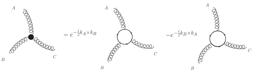
Figure 1: Color structure of three-gluon vertex of noncommutative $U(N)$ Yang-Mills theory in double line notation. The order of generators in trace strings are represented by the direction of arrows, and overall factor has been stripped off.

Similar difference exists in four-gluon vertex, where from Feynman rules we can see that for each such four-gluon vertex the color generators appear as[34]

tr $$\Big{[}\left(-i\cos(-{1\over 2}k_{A}\times k_{B})[t^{A},t^{B}]+\sin(-{1\over 2}k_{A}\times k_{B})\{t^{A},t^{B}\}\right)$$

$$\times\left(-i\cos(-{1\over 2}k_{C}\times k_{D})[t^{C},t^{D}]+\sin(-{1\over 2}k_{C}\times k_{D})\{t^{C},t^{D}\}\right)\Big{]}~{}.~{}~{}~{}$$

With the same trick we can reorganize this expression as

$$-e^{-{i\over 2}(k_{A}\times k_{B}+k_{C}\times k_{D})}\mbox{tr}(t^{A}t^{B}t^{C}t^{D})+e^{-{i\over 2}(k_{A}\times k_{B}-k_{C}\times k_{D})}\mbox{tr}(t^{A}t^{B}t^{D}t^{C})$$

$$+e^{{i\over 2}(k_{A}\times k_{B}-k_{C}\times k_{D})}\mbox{tr}(t^{B}t^{A}t^{C}t^{D})-e^{{i\over 2}(k_{A}\times k_{B}+k_{C}\times k_{D})}\mbox{tr}(t^{B}t^{A}t^{D}t^{C})~{},~{}~{}~{}~{}$$ (11)

and we can further use momentum conservation $k_{D}=-(k_{A}+k_{B}+k_{C})$ for the first and third phase factors and $k_{C}=-(k_{A}+k_{B}+k_{D})$ for the second and fourth phase factors to express them in a more systematic way. Combined with the property that $\theta^{\mu\nu}$ is antisymmetric, we have the following result

$$-e^{-{i\over 2}(k_{A}\times k_{B}+k_{A}\times k_{C}+k_{B}\times k_{C})}\mbox{tr}(t^{A}t^{B}t^{C}t^{D})+e^{-{i\over 2}(k_{A}\times k_{B}+k_{A}\times k_{D}+k_{B}\times k_{D})}\mbox{tr}(t^{A}t^{B}t^{D}t^{C})$$

$$+e^{-{i\over 2}(k_{B}\times k_{A}+k_{B}\times k_{C}+k_{A}\times k_{C})}\mbox{tr}(t^{B}t^{A}t^{C}t^{D})-e^{-{i\over 2}(k_{B}\times k_{A}+k_{B}\times k_{D}+k_{A}\times k_{D})}\mbox{tr}(t^{B}t^{A}t^{D}t^{C})~{}.~{}~{}~{}~{}$$ (12)

We see again that phase factors arise before color-ordered trace strings and the value of phase depends on the color order. In double line notation this color structure of four-gluon vertex can be expressed as in Fig. 2.

There is another important relation about $t^{A}$ strings of $U(N)$ group. While some strings of $t^{A}$ are terminated by fundamental indices, we have

$$(t^{A})^{~{}\bar{\j}_{1}}_{i_{1}}(t^{A})^{~{}\bar{\j}_{2}}_{i_{2}}=\delta^{~{}\bar{\j}_{2}}_{i_{1}}\delta^{~{}\bar{\j}_{1}}_{i_{2}}~{}.~{}~{}~{}$$ (13)

This relation enables us to express tree-level amplitudes of many gluons, which are constructed by three-gluon and four-gluon vertices, into sum of color-ordered amplitudes.

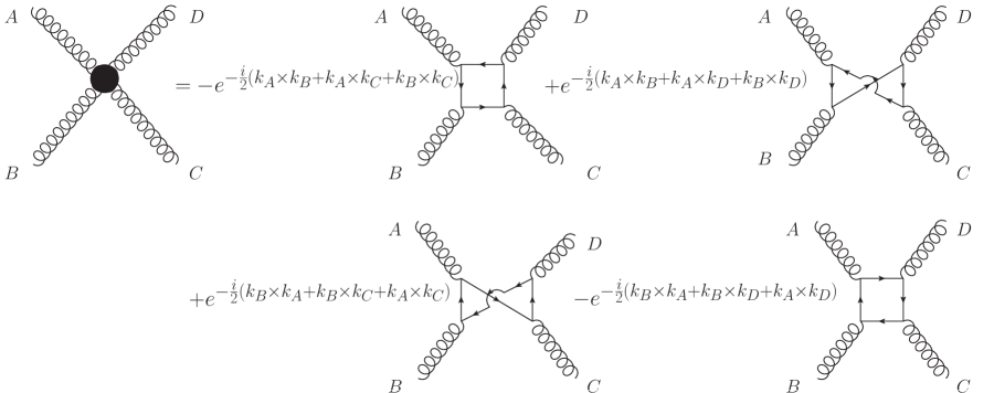
Figure 2: Color structure of four-gluon vertex of noncommutative $U(N)$ Yang-Mills theory in double line notation. The order of generators in trace strings are represented by the direction of arrows, and overall factor has been stripped off.

2.2 Color decomposition of noncommutative tree amplitudes

All these above observations lead to the consequence that one can write down the $n$-point tree amplitude as sum of single trace terms, i.e., color-ordered amplitudes, with additional phase factors. This is known as color decomposition of noncommutative scattering amplitudes. More explicitly, we have[8, 9, 10, 11, 36]

$$A^{tree}_{NC}(\{k_{i},\lambda_{i},a_{i}\})=g^{n-2}\sum_{\sigma\in S_{n}/Z_{n}}\mbox{tr}(t^{A_{\sigma(a)}}\dots t^{A_{\sigma(n)}})A^{tree}_{NC}(\sigma(1^{\lambda_{1}}),\ldots,\sigma(n^{\lambda_{n}}))~{},~{}~{}~{}~{}$$ (14)

where we have assumed that coupling constants of various vertices containing $SU(N)$ gluons and $U(1)$ gluons are the same and equal to $g$. $k_{i}$ and $\lambda_{i}$ are the gluon momenta and helicities, and $A_{NC}^{tree}$ are partial amplitudes of noncommutative $U(N)$ Yang-Mills theory which contain all the kinematic information and phase factors. $S_{n}$ is the set of all permutations of $n$ particles and $Z_{n}$ is the subset of cyclic permutations, which preserves the trace and should be eluded from summation in case of over counting. $A_{NC}^{tree}$ can be expressed explicitly as[37, 38, 39, 40, 41, 42, 32]

$$A_{NC}(k_{1},\ldots,k_{n})=A_{C}(k_{1},\ldots,k_{n})\phi(k_{1},\ldots,k_{n})~{},~{}~{}~{}$$ (15)

with phase factor

$$\phi(k_{1},\ldots,k_{n})=\exp\left[-{i\over 2}\sum_{1\leq i<j<n}k_{i}\times k_{j}\right]~{}.~{}~{}~{}$$ (16)

Since we will discuss only tree-level amplitudes in this note, the superscript of ”tree” has been thrown away for simplicity. The multiplication in phase factor is defined as $k_{i}\times k_{j}=k_{i}^{\mu}\theta_{\mu\nu}k_{j}^{\nu}$, and $A_{C}$ is color-ordered amplitude of conventional Yang-Mills theory.

2.3 Cyclic permutation and reflection of color order

Tree amplitudes of conventional field theory possess some nice properties which can be deduced directly from their color structure, such as color cyclic relation and reflection relation. In noncommutative $U(N)$ Yang-Mills theory, these relations might not be trivially held, since we should also consider the effect of phase factor after cyclic permutation or reflection. Let us first discuss cyclic permutation. The phase factor is invariant under cyclic permutation of gluons[32], which can be seen directly from its definition, i.e., if we relabel $k_{i}$ as $k_{i+1}$ and $k_{n}$ as $k_{1}$, then

$$\sum_{1\leq i<j<n}k_{i}\times k_{j}\to\sum_{2\leq i<j\leq n}k_{i}\times k_{j}=\sum_{2\leq i<j<n}k_{i}\times k_{j}+\sum_{2\leq i<n}k_{i}\times k_{n}~{},~{}~{}~{}$$ (17)

since $\sum_{2\leq i<n}k_{i}=-(k_{1}+k_{n})$ and $k_{n}=-\sum_{1\leq j<n}k_{j}$, and note that $k_{i}\times k_{i}=0$, the second term of (17) is just $\sum_{1<j<n}k_{1}\times k_{j}$. After combining this with the first term we reproduced the original phase factor, thus proved the cyclic property of phase factor. In this case, noncommutative tree amplitudes follow the same cyclic relation as amplitudes of conventional Yang-Mills theory, i.e.,

$$A_{NC}(k_{1},k_{2},\ldots,k_{n})=A_{NC}(k_{n},k_{1},\ldots,k_{n-1})~{}.~{}~{}~{}$$ (18)

Next let us discuss the color reflection relation of noncommutative Yang-Mills theory. When the color order is reversed, from the definition of phase factor we have

$$\phi(k_{n},\ldots,k_{1})=\exp\left[-{i\over 2}\sum_{n\geq i>j>1}k_{i}\times k_{j}\right]=\exp\left[{i\over 2}\sum_{1<j<i\leq n}k_{j}\times k_{i}\right]~{},~{}~{}~{}$$ (19)

where in the second step we used the antisymmetric property of $\theta^{\mu\nu}$, so that $k_{i}\times k_{j}=-k_{j}\times k_{i}$. The result is nothing but $\phi^{-1}(k_{2},\ldots,k_{n},k_{1})$, which we have shown before. Then use the property that phase factor is invariant under cyclic permutation we get

$$\phi(k_{n},\ldots,k_{1})=\phi^{-1}(k_{1},\ldots,k_{n})~{}.~{}~{}~{}~{}$$ (20)

This is the color reflection relation of phase factor. Using relation (15) and the known color reflection relation of conventional Yang-Mills theory, we can deduce the color reflection relation of noncommutative $U(N)$ Yang-Mills theory, i.e.,

$$A_{NC}(k_{n},\ldots,k_{1})=(-1)^{n}A_{NC}(k_{1},\ldots,k_{n})\phi^{-2}(k_{1},\ldots,k_{n})~{}.~{}~{}~{}$$ (21)

3 BCFW recursion relation

Since any amplitudes can be decomposed into color-ordered amplitudes, we could only focus on these color-ordered amplitudes. Is there an efficient method to compute these amplitudes? Or is there a way to analyze these color-ordered amplitudes without knowing their explicit expressions? We know that BCFW recursion relation can be served as a good answer to these problems. In this section we will try to extend BCFW recursion relation to noncommutative $U(N)$ Yang-Mills theory.

3.1 BCFW recursion relation for noncommutative $U(N)$ Yang-Mills theory

We have already seen from (15) that tree-level amplitudes of noncommutative Yang-Mills theory differ from amplitudes of conventional Yang-Mills theory in additional phase factors[37, 38, 39, 40, 41, 42, 32], so when discussing the validation of BCFW recursion relation of noncommutative Yang-Mills theory, we should focus on the discussion of phase factor. Let us first consider the following property of phase factor[37]

$$\phi(k_{1},\ldots,k_{n})=\phi(k_{1},\ldots,k_{m},P)\phi(-P,k_{m+1},\ldots,k_{n})~{},~{}~{}~{}$$ (22)

which is nothing but the relation of phase factors shown in Fig. 3. In other words, the product of two phase factors of sub-amplitudes, which are connected by a propagator, equals to the phase factor of a single amplitude of the left hand side of figure 3.

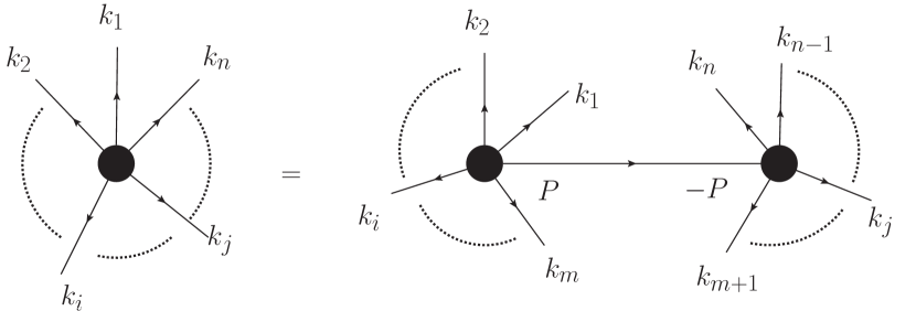
Figure 3: Phase factor of one single amplitude equals to the product of phase factors of two sub-amplitudes.

All external momenta are going outward so that momentum conservation takes the form $\sum_{1\leq i\leq n}k_{i}=0$, and the momentum of propagator is $P=-\sum_{1\leq i\leq m}k_{i}$. To prove this property, let us write down the phase factor as

$$\phi(k_{1},\ldots,k_{n}) = \exp\left[-{i\over 2}\sum_{1\leq i<j<n}k_{i}\times k_{j}\right]=\exp\left[-{i\over 2}\sum_{1\leq i<j\leq n}k_{i}\times k_{j}\right]$$

$$= \exp\left[-{i\over 2}\sum_{1\leq i<j\leq m}k_{i}\times k_{j}-{i\over 2}\sum_{\begin{subarray}{c}1\leq i\leq m\\ m+1\leq j\leq n\end{subarray}}k_{i}\times k_{j}-{i\over 2}\sum_{m+1\leq i<j\leq n}k_{i}\times k_{j}\right]~{}.~{}~{}~{}$$

The first line is true because $\sum_{1\leq i<n}k_{i}\times k_{n}=-k_{n}\times k_{n}=0$. Let us deal with those three terms in the second line. The first term is $\phi(k_{1},\ldots,k_{m},P)$ by definition. The second term is zero since $\sum_{1\leq i\leq m}k_{i}=-P$ and $\sum_{m+1\leq j\leq n}k_{j}=P$, so the summation equals to $-P\times P=0$. The third term is $\phi(k_{m+1},\ldots,k_{n},-P)$ by definition, and because of cyclic relation of phase factor this is just $\phi(-P,k_{m+1},\ldots,k_{n})$. This proved relation (22). Note that we use only momentum conservation and antisymmetric property of $\theta^{\mu\nu}$ through the proof, and BCFW deformation of two selected momenta will always keep momentum conversation, so the above argument is also held when momenta are shifted.

Then let us discuss BCFW shifting of $n$-point noncommutative amplitude. We pick up two momenta $k_{i},k_{j}$ and take following shifting

$$\hat{k}_{i}=k_{i}-z\tilde{q}~{},~{}~{}~{}\hat{k}_{j}=k_{j}+z\tilde{q}~{}.~{}~{}~{}$$ (23)

Amplitudes of conventional Yang-Mills theory are often written down in spinor formalism so that they have more compact and elegant form (see [11] and references there in). In spinor formalism $\tilde{q}$ is often taken as $\tilde{q}_{a\dot{a}}=\lambda_{ia}\tilde{\lambda}_{j\dot{a}}$, so that $\tilde{q}^{2}=\tilde{q}\cdot k_{i}=\tilde{q}\cdot k_{j}=0$, and $\hat{k}_{i},\hat{k}_{j}$ are on-shell. We can always change $\tilde{q}_{a\dot{a}}$ back to $\tilde{q}^{\mu}$ with $\sigma^{\mu a\dot{a}}$ matrix. Tree amplitudes of noncommutative Yang-Mills theory contain two parts, one is phase factor and the other is the amplitude of conventional field theory. Since here we want to discuss the effect of phase factor after BCFW shifting, we will assume that for amplitude of conventional Yang-Mills theory this shifting always leads to correct boundary condition[44, 45, 46, 47]. Then after taking $(k_{i},k_{j})$-shifting the phase factor becomes

$$\phi(k_{1},\ldots,\hat{k}_{i},\ldots,\hat{k}_{j},\ldots,k_{n})=\phi(k_{1},\ldots,k_{n})\varphi(z)~{},~{}~{}~{}$$ (24)

where

$$\varphi(z)=\exp\left[-z{i\over 2}\left(k_{i}+2\sum_{i<l<j}k_{l}+k_{j}\right)\times\tilde{q}\right]~{}.~{}~{}~{}$$ (25)

We see that phase factor is not invariant after $(k_{i},k_{j})$-shifting and $z$-dependence enters into phase factor through $\varphi(z)$. It is obviously that $\varphi(z)$ would not equal to one if $z\neq 0$, since $(k_{i}+2\sum_{i<l<j}k_{l}+k_{j})\times\tilde{q}$ does not necessary vanish. In fact, result of $(k_{i}+2\sum_{i<l<j}k_{l}+k_{j})\times\tilde{q}$ depends not only on the way of shifting but also on the value of $\theta^{\mu\nu}$. Is there a suitably chosen $\tilde{q}$ that satisfies both requirements of BCFW deformation and the vanishing of above result? It seems not possible in 4-dimension space-time. $\tilde{q}$ is chosen that $\tilde{q}\cdot k_{i}=\tilde{q}\cdot k_{j}=\tilde{q}^{2}=0$, and these requirements are satisfied only when auxiliary momentum $\tilde{q}$ is complex[44]. More explicitly, since $k_{i}$ and $k_{j}$ are massless, we could choose a suitable frame so that $k_{i}=(E,E,0,0),k_{j}=(E,-E,0,0)$, and assume $\tilde{q}=(E_{q},q_{x},q_{y},q_{z})$. Two equations $k_{i}\cdot\tilde{q}=k_{j}\cdot\tilde{q}=0$ will determine two components of $\tilde{q}$, and in the chosen frame we have $E_{q}=q_{x}=0$. The massless condition of $\tilde{q}$ gives one more constraint on $\tilde{q}$ and we have $q_{y}^{2}+q_{z}^{2}=0$. Then requirement of $(k_{i}+2\sum_{i<l<j}k_{l}+k_{j})\times\tilde{q}=0$ adds one more linear constraint on $\tilde{q}$ so that $aq_{y}+bq_{z}=0$, and $a,b$ are certain real constants. The solution of these two constraints is $q_{y}=q_{z}=0$. In this case auxiliary momentum $\tilde{q}$ is just a null vector, so we see that there are no non-trivial solution of $\tilde{q}$ that satisfies all these requirements.

What is the problem if phase factor after shifting is not equal to phase factor that are not being shifted? Generally speaking, we would expect that BCFW recursion relation of noncommutative $U(N)$ Yang-Mills theory takes the same form as conventional Yang-Mills theory, i.e.,

$$A_{NC}(k_{1},\ldots,k_{n})=\sum_{P_{ab}}A_{NC}^{h}(\ldots,\hat{k}_{i}(z_{ab}),\ldots,\hat{P}_{ab}(z_{ab})){1\over P_{ab}^{2}}A_{NC}^{-h}(-\hat{P}_{ab}(z_{ab})\ldots,\hat{k}_{j}(z_{ab}),\ldots)~{},~{}~{}~{}$$ (26)

where summation is over all possible helicities and propagators, and $z_{ab}$ is the solution of $\hat{P}^{2}_{ab}(z)=0$. This is obviously not true from (15). The phase factor for left hand side of (26) is $\phi(k_{1},\ldots,k_{n})$. Each term of BCFW expansion in right hand side of (26) has a phase factor $\phi(k_{1},\ldots,\hat{k}_{i}(z_{ab}),\ldots,\hat{k}_{j}(z_{ab}),\ldots,k_{n})$, after using cyclic relation of phase factor and (22). So the phase factor in the left hand side of (26) does not equal to phase factors in the right hand side of (26), and even phase factors in the right hand side do not equal to each other.

In order to write down a suitable BCFW recursion relation for noncommutative $U(N)$ Yang-Mills theory, let us recall the supersymmetric BCFW recursion relation[15, 48, 49, 50]. We are forced to take $(k_{i},k_{j})$-shifting so that energy-momentum conservation is satisfied after shifting, and in supersymmetric BCFW recursion relation we are forced to take one more Grassmann variable $\eta$-shifting so that super-energy-momentum conservation is satisfied. In noncommutative case, the one that must be kept invariant is phase factor, so it is reasonable to consider taking some kind of phase-deformation. It is also natural to think this problem from the view of singularities. In tree amplitudes of noncommutative $U(N)$ Yang-Mills theory, there are so called essential singularities from phase factors and ordinary singularities from propagators. We could eliminate essential singularities by multiplying one additional phase factor, so that there are only ordinary singularities from propagators, and BCFW recursion relation is valid. More specifically, we have

$$A_{NC}(k_{1},\ldots,k_{n})\phi^{-1}(k_{1},\ldots,k_{n}) = \sum_{P_{ab}}\Big{[}A_{NC}^{h}(\ldots,\hat{k}_{i}(z_{ab}),\ldots,\hat{P}_{ab}(z_{ab}))\phi^{-1}(\ldots,\hat{k}_{i}(z_{ab}),\ldots,\hat{P}_{ab}(z_{ab}))$$

$$\times{1\over P_{ab}^{2}}A_{NC}^{-h}(-\hat{P}_{ab}(z_{ab})\ldots,\hat{k}_{j}(z_{ab}),\ldots)\phi^{-1}(-\hat{P}_{ab}(z_{ab})\ldots,\hat{k}_{j}(z_{ab}),\ldots)\Big{]}~{}.~{}~{}~{}$$

The above recursion relation can be further simplified by multiplying $\phi(k_{1},\ldots,k_{n})$ in both left hand side and right hand side. Using (22) and cyclic relation of phase factor we have

$$\phi^{-1}(\ldots,\hat{k}_{i}(z_{ab}),\ldots,\hat{P}_{ab}(z_{ab}))\phi^{-1}(-\hat{P}_{ab}(z_{ab})\ldots,\hat{k}_{j}(z_{ab}),\ldots)=\phi^{-1}(k_{1},\ldots,\hat{k}_{i}(z_{ab}),\ldots,\hat{k}_{j}(z_{ab}),\ldots,k_{n})~{},~{}~{}~{}$$ (28)

and after using (24) we have

$$\phi(k_{1},\ldots,k_{n})\phi^{-1}(k_{1},\ldots,\hat{k}_{i}(z_{ab}),\ldots,\hat{k}_{j}(z_{ab}),\ldots,k_{n})=\varphi^{-1}(z_{ab})~{},~{}~{}~{}$$ (29)

where $\varphi(z)$ is defined in (25). Then we have

$$A_{NC}(k_{1},\ldots,k_{n})=\sum_{P_{ab}}A_{NC}^{h}(\ldots,\hat{k}_{i}(z_{ab}),\ldots,\hat{P}_{ab}(z_{ab})){\varphi^{-1}(z_{ab})\over P_{ab}^{2}}A_{NC}^{-h}(-\hat{P}_{ab}(z_{ab})\ldots,\hat{k}_{j}(z_{ab}),\ldots)~{}.~{}~{}~{}$$ (30)

Since essential singularities have been removed from amplitudes of noncommutative Yang-Mills theory in BCFW recursion relation (30), there would be no problems considering singularities or large $z$ behavior of $A_{NC}$ in complex plane as long as BCFW recursion relation of conventional field theory is held. Of course (30) is not the best way to compute tree amplitudes of noncommutative $U(N)$ Yang-Mills theory. Thanks to relation (15), in order to get amplitudes of noncommutative Yang-Mills theory, we can simply obtain tree amplitudes of conventional field theory by ordinary BCFW recursion relation and multiply them with corresponding phase factors. But recursion relation (30) could be served as a good tool for noncommutative theory in S-Matrix program where, for example, one may want to prove some identities of amplitudes without knowing explicit expressions of these amplitudes, etc.

3.2 Three-point amplitudes

The on-shell BCFW recursion relation allows us to construct any tree amplitudes from three-point amplitudes theoretically. After writing down BCFW recursion relation for noncommutative Yang-Mills theory, we further want to get noncommutative three-point amplitudes. Three-point amplitudes are fundamental amplitudes, but we know that there are no three-point scattering amplitudes when all three momenta are real[14, 15, 16, 17]. In order to satisfy energy-momentum conservation and massless conditions, we have $p_{i}\cdot p_{j}=0$ for any momenta. In spinor formalism these equations are $\left\langle i~{}j\right\rangle\left[i~{}j\right]=0$, which means that either $\left\langle i~{}j\right\rangle=0$ or $\left[i~{}j\right]=0$ if complex momenta are allowed, so the three-point amplitudes are purely holomorphic or anti-homomorphic. In conventional field theory it is known that for particles of spin $s$, the amplitudes of helicity configurations $(+,+,-)$ and $(-,-,+)$ should be of the form

$$A^{--+}=\left({\left\langle 1~{}2\right\rangle^{4}\over\left\langle 1~{}2\right\rangle\left\langle 2~{}3\right\rangle\left\langle 3~{}1\right\rangle}\right)^{s}~{},~{}~{}~{}~{}A^{++-}=\left({\left[1~{}2\right]^{4}\over\left[1~{}2\right]\left[2~{}3\right]\left[3~{}1\right]}\right)^{s}~{}.~{}~{}~{}~{}$$ (31)

These forms are determined up to an overall dimensionless coupling constant[15]. To construct three-point amplitudes of noncommutative field theory we could naively add one additional phase factor on (31). For noncommutative $U(N)$ Yang-Mills theory we conclude that

$$A_{NC}(1^{-},2^{-},3^{+})=e^{-{i\over 2}k_{1}\times k_{2}}\left({\left\langle 1~{}2\right\rangle^{4}\over\left\langle 1~{}2\right\rangle\left\langle 2~{}3\right\rangle\left\langle 3~{}1\right\rangle}\right)~{},~{}~{}~{}~{}A_{NC}(1^{+},2^{+},3^{-})=e^{-{i\over 2}k_{1}\times k_{2}}\left({\left[1~{}2\right]^{4}\over\left[1~{}2\right]\left[2~{}3\right]\left[3~{}1\right]}\right)~{}.~{}~{}~{}$$ (32)

Due to energy-momentum conservation and antisymmetry of $\theta^{\mu\nu}$ we have $k_{1}\times k_{2}=k_{2}\times k_{3}=k_{3}\times k_{1}$, thus the phase factor can be written in other equivalent forms. Different from conventional field theory, we have an additional parameter $\theta^{\mu\nu}$ in noncommutative Yang-Mills theory and this parameter enables us to construct dimensionless constant from momenta. For example the multiplication $k_{i}\times k_{j}$ is dimensionless, and phase factors (32) are also dimensionless. Then forms of (32) are determined up to overall coupling constant and dimensionless constants constructed from $\theta^{\mu\nu}$. It would be an interesting work to discuss consistency conditions on the S-matrix of noncommutative field theory.

There is one property of three-point amplitudes we want to address. By direct verification we see that

$$A_{NC}(k_{1},k_{2},k_{3})=-A_{NC}(k_{3},k_{2},k_{1})\phi^{-2}(k_{3},k_{2},k_{1})~{}.~{}~{}~{}$$ (33)

This relation can be considered as a special case of color reflection relation (21) when $n=3$. It is simple to prove (21) by BCFW recursion relation of noncommutative Yang-Mills theory starting from three-point relation (33), and (33) will play an important role in the later demonstration of amplitude relations of noncommutative Yang-Mills theory.

3.3 A simple example: computing four-point amplitude $A_{NC}(1^{+},2^{+},3^{-},4^{-})$

As a verification of these three-point amplitudes and noncommutative BCFW recursion relation, a simple example will be given below to show how to construct four-point amplitude from three-point amplitudes. Let us consider four-point amplitude of helicity configuration $(++--)$. We will take $(k_{1},k_{4})$-shifting, i.e.,

$$\hat{k}_{1}=k_{1}-z\tilde{q}~{},~{}~{}~{}\hat{k}_{4}=k_{4}+z\tilde{q}~{},~{}~{}~{}$$ (34)

and in the spinor formalism we have $\tilde{q}=|4\rangle|1]$. Consequently we have shifted the holomorphic part of $k_{1}$ and the anti-holomorphic part of $k_{4}$. According to (30) we have

$$A_{NC}(1^{+},2^{+},3^{-},4^{-})=A_{NC}(\hat{1}^{+},2^{+},-\hat{P}^{-}){\exp[z_{14}{i\over 2}(k_{1}+2(k_{2}+k_{3})+k_{4})\times\tilde{q}]\over s_{12}}A_{NC}(\hat{P}^{+},3^{-},\hat{4}^{-})~{},~{}~{}~{}$$ (35)

where $\hat{P}=\hat{k}_{1}+k_{2}$ and $z_{14}$ is the solution of $\hat{P}^{2}=0$, and $s_{12}=(k_{1}+k_{2})^{2}$ is the propagator. In order to get $z_{14}$ we should solve equation

$$\hat{P}^{2}=\left\langle 1~{}2\right\rangle\left[1~{}2\right]-z\left\langle 2~{}4\right\rangle\left[2~{}1\right]=0~{},~{}~{}~{}$$ (36)

and the result is

$$z_{14}=-{\left\langle 1~{}2\right\rangle\over\left\langle 2~{}4\right\rangle}~{}.~{}~{}~{}$$ (37)

The three-point sub-amplitudes can be written down directly as

$$A_{NC}(\hat{1}^{+},2^{+},-\hat{P}^{-})=e^{-{i\over 2}\hat{k}_{1}\times k_{2}}{\left[1~{}2\right]^{4}\over\left[1~{}2\right][2~{}\hat{P}][\hat{P}~{}1]}~{},~{}~{}~{}~{}A_{NC}(\hat{P}^{+},3^{-},\hat{4}^{-})=e^{-{i\over 2}k_{3}\times\hat{k}_{4}}{\left\langle 3~{}4\right\rangle^{4}\over\langle\hat{P}~{}3\rangle\left\langle 3~{}4\right\rangle\langle 4~{}\hat{P}\rangle}~{}.~{}~{}~{}$$ (38)

Firstly let us compute the phase factor in right hand side of (35), which is

$$\exp\left[-{i\over 2}\left(k_{1}\times k_{2}-z_{14}\tilde{q}\times k_{2}-z_{14}(k_{1}+2(k_{2}+k_{3})+k_{4})\times\tilde{q}+k_{3}\times k_{4}+z_{14}k_{3}\times\tilde{q}\right)\right]$$

$$= \exp\left[-{i\over 2}(k_{1}\times k_{2}+k_{3}\times k_{4}-z_{14}(k_{1}+k_{2}+k_{3}+k_{4})\times\tilde{q})\right]$$

$$= \exp\left[-{i\over 2}(k_{1}\times k_{2}+k_{1}\times k_{3}+k_{2}\times k_{3})\right]\equiv\phi(1,2,3,4)~{},~{}~{}~{}$$

where we have used $k_{4}=-(k_{1}+k_{2}+k_{3})$ and antisymmetry of $\theta^{\mu\nu}$ in the second step. Then we want to compute

$${\left[1~{}2\right]^{4}\over\left[1~{}2\right][2~{}\hat{P}][\hat{P}~{}1]}{1\over s_{12}}{\left\langle 3~{}4\right\rangle^{4}\over\langle\hat{P}~{}3\rangle\left\langle 3~{}4\right\rangle\langle 4~{}\hat{P}\rangle} = {\left[1~{}2\right]^{3}\left\langle 3~{}4\right\rangle^{3}\over s_{12}[2|\hat{P}|3\rangle[1|\hat{P}|4\rangle}~{}.~{}~{}~{}$$

Since $\hat{P}=|1\rangle|1]+|2\rangle|2]-z_{14}|4\rangle|1]$ it is easy to see that

$$[1|\hat{P}|4\rangle = \left[1|2|4\right\rangle~{},~{}~{}~{}$$

and

$$[2|\hat{P}|3\rangle = \left[2|1|3\right\rangle-z_{14}\left[2~{}1\right]\left\langle 4~{}3\right\rangle$$

$$= {\left[2~{}1\right]\over\left\langle 2~{}4\right\rangle}\left(\left\langle 2~{}4\right\rangle\left\langle 1~{}3\right\rangle+\left\langle 1~{}2\right\rangle\left\langle 4~{}3\right\rangle\right)$$

$$= {\left[2~{}1\right]\left\langle 2~{}3\right\rangle\left\langle 1~{}4\right\rangle\over\left\langle 2~{}4\right\rangle}~{},~{}~{}~{}$$

where we have used Schouten identity in the second step. By writing $s_{12}=\left\langle 1~{}2\right\rangle\left[1~{}2\right]$ and put all the above results back to (35) we get the final result

$$A_{NC}(1^{+},2^{+},3^{-},4^{-})={\left\langle 3~{}4\right\rangle^{4}\over\left\langle 1~{}2\right\rangle\left\langle 2~{}3\right\rangle\left\langle 3~{}4\right\rangle\left\langle 4~{}1\right\rangle}\phi(1,2,3,4)~{}.~{}~{}~{}$$ (39)

This result is same as the one obtained from (15).

4 Relations of amplitudes in noncommutative $U(N)$ Yang-Mills theory

We know that any tree amplitudes can be expressed as sum of color-ordered amplitudes, and there is so called BCFW recursion relation which can be used to efficiently compute or analyze these amplitudes. But thanks to some nontrivial relations of amplitudes we do not need to calculate all these color-ordered amplitudes. In noncommutative $U(N)$ Yang-Mills theory, there are also analogies of these nontrivial relations. In this section, we will write down the analogies of $U(1)$-decoupling, KK and BCJ relations in noncommutative Yang-Mills theory and prove them with BCFW recursion relation of noncommutative version recursively, starting from the verified three-point relations.

4.1 Modified $U(1)$-decoupling relation

In conventional $U(N)$ Yang-Mills theory, $U(1)$ gauge boson is identified as photon, and $SU(N)$ as gluons. Since any amplitude containing extra $U(1)$ photon must vanish and $U(1)$ generator commutes with other generators, we could get $U(1)$-decoupling relation. But in noncommutative $U(N)$ Yang-Mills theory there are interactions among $U(1)$ gluons and $SU(N)$ gluons[34], so amplitude containing $U(1)$ gluons exists, and we could not get similar $U(1)$-decoupling relation of $A_{NC}$ by simply replacing $A_{C}$ with $A_{NC}$ in ordinary $U(1)$-decoupling relation. So a modified $U(1)$-decoupling relation is necessary for tree amplitudes of noncommutative Yang-Mills theory. It is reasonable to infer that phase factor would appear in noncommutative $U(1)$-decoupling relation, since phase factor is a character of noncommutative Yang-Mills theory. In fact, deduced from (15) we could get the noncommutative $U(1)$-decoupling relation

$$\sum_{\sigma\in~{}cyclic}A_{NC}(k_{1},\sigma(k_{2},\ldots,k_{n}))\phi^{-1}(k_{1},\sigma(k_{2},\ldots,k_{n}))=0~{},~{}~{}~{}$$ (40)

where $\sigma$ is the set of cyclic permutation of $(k_{2},\ldots,k_{n})$. The appearance of phase factor $\phi^{-1}$ is an effect of noncommutative space-time structure. In the limit that $\theta^{\mu\nu}\to 0$ the space-time turns to be normal, and $\phi^{-1}\to 1$ while $A_{NC}\to A_{C}$, thus noncommutative $U(1)$-decoupling relation (40) turns to ordinary $U(1)$-decoupling relation of gauge theory.

The $U(1)$-decoupling relation of three-point is

$$A_{NC}(k_{1},k_{2},k_{3})\phi^{-1}(k_{1},k_{2},k_{3})+A_{NC}(k_{1},k_{3},k_{2})\phi^{-1}(k_{1},k_{3},k_{2})=0~{}.~{}~{}~{}$$ (41)

Through cyclic relation (18) we have $A_{NC}(k_{1},k_{3},k_{2})=A_{NC}(k_{3},k_{2},k_{1})$, and using the color reflection relation of phase factor, i.e., $\phi(k_{1},k_{2},k_{3})=\phi^{-1}(k_{3},k_{2},k_{1})$, we can rewrite the above relation as

$$A_{NC}(k_{1},k_{2},k_{3})=-A_{NC}(k_{3},k_{2},k_{1})\phi^{-2}(k_{3},k_{2},k_{1})~{}.~{}~{}~{}$$ (42)

This is the three-point relation (33) we have verified. We want to prove $U(1)$-decoupling relation of general point recursively through BCFW recursion relation of noncommutative Yang-Mills theory (30). Suppose noncommutative $U(1)$-decoupling relation is satisfied by all noncommutative tree amplitudes less than $n$-point, we will demonstrate that it is true for $n$-point tree amplitude.

We can rewrite the $n$-point noncommutative $U(1)$-decoupling relation as

$$\sum_{\sigma\in cyclic}A_{NC}(1,\sigma(2,3,\ldots,n))\phi^{-1}(1,\sigma(2,3,\ldots,n))=0~{}.~{}~{}~{}~{}$$ (43)

For expression simplicity we introduce split notation $|$, which is defined as

$$A_{NC}(\hat{1},\ldots,i|i+1,\ldots,\hat{n})\equiv\sum_{h}A_{NC}(\hat{1},\ldots,i,\hat{P}_{1i}^{h}){1\over P_{1i}^{2}}A_{NC}(-\hat{P}^{-h}_{1i},i+1,\ldots,\hat{n})~{}.~{}~{}~{}~{}$$ (44)

In this notation, we expand every amplitude in (43) using BCFW expansion under $(n-1,n)$-shifting, for example

$$A_{NC}(1,2,\ldots,n-1,n)=\sum_{i=1}^{n-3}A_{NC}(\hat{n},1,\ldots,i|i+1,\ldots,n-2,\widehat{n-1})\varphi^{-1}(z_{n1\cdots i})~{},~{}~{}~{}$$ (45)

where $\varphi(z)$ is

$$\varphi(z)=\exp\Big{[}z{i\over 2}(k_{n}+k_{n-1})\times\tilde{q}\Big{]}~{},~{}~{}~{}$$ (46)

and $z_{n1\cdots i}$ is the solution of $\hat{P}^{2}=(\hat{k}_{n}+k_{1}+\cdots+k_{i})^{2}=0$. Note that under different manners of shifting $z_{n1\cdots i}$ will take different values. For example, we can take $\left\langle n-1|n\right]$-shifting or $\left\langle n|n-1\right]$-shifting under $(n-1,n)$-shifting, and $z_{n1\cdots i}$ is different under these two manners of shifting. But this property will not affect the proof, since this proof is general and does not depend on the details of BCFW shifting.

We also have

$$A_{NC}(1,n-1,n,2,\ldots,n-3,n-2)=\sum_{i=2}^{n-2}A_{NC}(\hat{n},2,\ldots,i|i+1,\ldots,n-2,1,\widehat{n-1})\varphi^{-1}(z_{n2\cdots i})~{},~{}~{}~{}$$ (47)

where $z_{n2\cdots i}$ is determined by the equation $(\hat{k}_{n}+k_{2}+k_{3}+\cdots+k_{i})^{2}=0$. Another two special cases are

$$A_{NC}(1,n,2,\ldots,n-2,n-1) = \sum_{i=2}^{n-2}A_{NC}(\hat{n},2,\ldots,i|i+1,\ldots,n-2,\widehat{n-1},1)\varphi^{-1}(z_{n2\cdots i})$$ (48)

$$+ \sum_{i=2}^{n-2}A_{NC}(1,\hat{n},2,3,\ldots,i-1|i,\ldots,n-2,\widehat{n-1})\varphi^{-1}(z_{n1\cdots i-1})~{},~{}~{}~{}$$

and

$$A_{NC}(1,3,4,\ldots,n-1,n,2) = A_{NC}(\hat{n},2|1,3,\ldots,n-2,\widehat{n-1})\varphi^{-1}(z_{n2})$$ (49)

$$+ \sum_{i=3}^{n-2}A_{NC}(\hat{n},2,1,3,\ldots,i-1|i,\ldots,n-2,\widehat{n-1})\varphi^{-1}(z_{n1\cdots i-1})~{}.~{}~{}~{}$$

For other general cases $(4\leqslant j\leqslant n-2)$, we have

$$A_{NC}(1,j,\ldots,n,2,\ldots,j-1) = \sum_{i=2}^{j-1}A_{NC}(\hat{n},2,3,\ldots,i|i+1,\ldots,j-1,1,j,\ldots,n-2,\widehat{n-1})\varphi^{-1}(z_{n2\cdots i})$$ (50)

$$+ \sum_{i=j}^{n-2}A_{NC}(\hat{n},2,\ldots,j-1,1,j,\ldots,i-1|i,\ldots,\widehat{n-1})\varphi^{-1}(z_{n1\cdots i}).$$

In the above expansions, we have ignored phase factors in (43). Let us take them back and consider the general case (50). According to (24), we have

$$\varphi^{-1}(z_{n2\cdots i})\phi^{-1}(1,j,\ldots,n,2,\ldots,j-1)$$ (51)

$$= \varphi^{-1}(z_{n2\cdots i})\phi^{-1}(n,2,3,\ldots,i,i+1,\ldots,j-1,1,j,\ldots,n-2,n-1)$$

$$= \phi^{-1}(\hat{n}(z_{n2\cdots i}),2,3,\ldots,i,i+1,\ldots,j-1,1,j,\ldots,n-2,\widehat{n-1}(z_{n2\cdots i}))$$

$$= \phi^{-1}(\hat{n}(z_{n2\cdots i}),2,3,\ldots,i,\hat{P}_{n2\cdots i})\phi^{-1}(-\hat{P}_{n2\cdots i},i+1,\ldots,j-1,1,j,\ldots,n-2,\widehat{n-1}(z_{n2\cdots i}))~{}.~{}~{}~{}$$

Similar operation can be applied to $\varphi^{-1}(z_{n1\cdots i})$ and phases in the special cases. We see that all the expansions can be divided into two groups: one contains parameter $z_{n2\cdots i}$, and the other contains $z_{n1\cdots i}$. Firstly, let us consider all terms containing $z_{n2\cdots i}$, and we can arrange them as follows,

$$A_{NC}(\hat{n},2|1,3,\ldots,n-2,\widehat{n-1})\varphi^{-1}(z_{n2})\phi^{-1}(n,2,1,3,\ldots,n-1)$$ (52)

$$+ \sum_{j=4}^{n-2}\sum_{i=2}^{j-1}A_{NC}(\hat{n},2,3,\ldots,i|i+1,\ldots,j-1,1,j,\ldots,n-2,\widehat{n-1})\varphi^{-1}(z_{n2\cdots i})\phi^{-1}(n,2,\ldots,j,1,j+1,\ldots,n-1)$$

$$+ \sum_{i=2}^{n-2}A_{NC}(\hat{n},2,\ldots,i|i+1,\ldots,n-2,1,\widehat{n-1})\varphi^{-1}(z_{n2\cdots i})\phi^{-1}(n,2,\ldots,n-2,1,n-1)$$

$$+ \sum_{i=2}^{n-2}A_{NC}(\hat{n},2,\ldots,i|i+1,\ldots,n-2,\widehat{n-1},1)\varphi^{-1}(z_{n2\cdots i})\phi^{-1}(n,2,\ldots,n-1,1)~{}.~{}~{}~{}$$

Then according to (51) we can obtain terms as

$$\sum_{h}\Big{[}A_{NC}(\hat{n},2,\ldots,i,\hat{P}^{h}_{n2\cdots i})\phi^{-1}(\hat{n}(z_{n2\cdots i}),2,3,\ldots,i,\hat{P}^{h}_{n2\cdots i}){1\over P_{n2\cdots i}^{2}}$$

$$\times\sum_{\sigma\in cyclic}A_{NC}(-\hat{P}^{-h}_{n2\cdots i},\sigma(1,i+1,\ldots,n-2,\widehat{n-1}))\phi^{-1}(-\hat{P}^{-h}_{n2\cdots i},\sigma(1,i+1,\ldots,n-2,\widehat{n-1}))\Big{]}~{}.~{}~{}~{}$$ (53)

Using $(n-i+1)$-point noncommutative $U(1)$-decoupling relation, we see the above summation vanishes. So all terms containing $z_{n2\cdots i}$ are zero. The same argument holds for all terms containing $z_{n1\cdots i}$. Thus we proved the noncommutative $U(1)$-decoupling relation for $n$-point tree amplitudes.

4.2 Noncommutative KK relations

General KK relations should also be modified to fit the requirement of noncommutative Yang-Mills theory, and we conclude that noncommutative KK relations take the form

$$A_{NC}(1,\{{\alpha}\},n,\{{\beta}\})\phi^{-1}(1,\{{\alpha}\},n,\{{\beta}\})=(-1)^{n_{\beta}}\sum_{\sigma\in OP(\{{\alpha}\},\{{\beta}^{T}\})}A_{NC}(1,\sigma,n)\phi^{-1}(1,\sigma,n)~{}.~{}~{}~{}~{}$$ (54)

where $OP(\{{\alpha}\},\{{\beta}^{T}\})$ is the ordered permutations between sets $\{{\alpha}\}$ and $\{{\beta}^{T}\}$, i.e., the permutation keeps order of set $\{{\alpha}\}$ and set $\{{\beta}^{T}\}$. $\{{\beta}^{T}\}$ is the reverse ordering of $\{{\beta}\}$.

Let us consider a special case that $\{{\alpha}\}$ is empty. The KK relations become

$$A_{NC}(1,n,\{{\beta}\})\phi^{-1}(1,n,\{{\beta}\}) = (-1)^{n_{\beta}}A_{NC}(1,\{{\beta}^{T}\},n)\phi^{-1}(1,\{{\beta}^{T}\},n)$$ (55)

$$= (-1)^{n_{\beta}}A_{NC}(\{{\beta}^{T}\},n,1)\phi^{-1}(\{{\beta}^{T}\},n,1)~{}.~{}~{}~{}$$

Using color reflection relation for phase factor, we have

$$\phi^{-1}(1,n,\{{\beta}\})=\phi(\{{\beta}^{T}\},n,1)~{}.~{}~{}~{}$$ (56)

Then we get $(n_{\beta}+2)$-point color reflection relation

$$A_{NC}(1,n,\{{\beta}\})=(-1)^{n_{\beta}}A_{NC}(\{{\beta}^{T}\},n,1)\phi^{-2}(\{{\beta}^{T}\},n,1).$$ (57)

Thus we see that noncommutative color reflection relation is a special case of noncommutative KK relations.

Then let us consider another special case when $\{{\beta}\}$ has only one element. In this case we have

$$A_{NC}(1,\{{\alpha}\},n,{\beta})\phi^{-1}(1,\{{\alpha}\},n,{\beta})=(-1)\sum_{OP}A_{NC}(1,OP(\{{\alpha}\}\cup{\beta}),n)\phi^{-1}(1,OP(\{{\alpha}\}\cup{\beta}),n)~{}.~{}~{}~{}$$ (58)

Since $A_{NC}$ and phase factors are invariant under cyclic permutations, the above equation become

$$A_{NC}(1,\{{\alpha}\},n,{\beta})\phi^{-1}(1,\{{\alpha}\},n,{\beta})+\sum_{OP}A_{NC}(1,OP(\{{\alpha}\}\cup{\beta}),n)\phi^{-1}(1,OP(\{{\alpha}\}\cup{\beta}),n)$$ (59)

$$= \sum_{\sigma\in cyclic}A_{NC}({\beta},\sigma(1,\{{\alpha}\},n))\phi^{-1}({\beta},\sigma(1,\{{\alpha}\},n))~{}.~{}~{}~{}$$

This is nothing but noncommutative $U(1)$-decoupling relation. It can be easily checked that the special case that $\{{\alpha}\}$ containing only one element is also noncommutative $U(1)$-decoupling relation.

After checking above several special cases, we use noncommutative BCFW recursion relation to prove general noncommutative KK relations, which is

$$A_{NC}(1,\{{\alpha}_{1},\ldots,{\alpha}_{l}\},n,\{{\beta}_{1},\ldots,{\beta}_{m}\})\phi^{-1}(1,\{{\alpha}_{1},\ldots,{\alpha}_{l}\},n,\{{\beta}_{1},\ldots,{\beta}_{m}\})$$ (60)

$$= (-1)^{m}\sum_{\sigma\in OP(\{{\alpha}\},\{{\beta}^{T}\})}A_{NC}(1,\sigma,n)\phi^{-1}(1,\sigma,n)~{}.~{}~{}~{}$$

We will use noncommutative BCFW recursion relation to expand tree amplitudes in both sides of KK relations. It can be shown that each term in the left hand side belongs to the right hand side and both sides have the same number of terms. For the right hand side of noncommutative KK relations, using BCFW recursion relation and $(n,1)$-shifting, we have

$$(-1)^{m}\sum_{\sigma\in OP(\{{\alpha}\},\{{\beta}^{T}\})}A_{NC}(1,\sigma,n)\phi^{-1}(1,\sigma,n)$$ (61)

$$= (-1)^{m}\sum_{\sigma\in OP(\{{\alpha}\},\{{\beta}^{T}\})}\sum_{h;i=1}^{l+m-1}A_{NC}(\hat{1},\sigma_{1},\ldots,\sigma_{i}|\sigma_{i+1},\ldots,\sigma_{l+m},\hat{n})\phi^{-1}(\hat{1},\sigma,\hat{n})~{}.~{}~{}~{}$$

The total number of terms in the above expansion is

$$\frac{(l+m)!}{l!m!}(l+m-1)~{}.~{}~{}~{}$$ (62)

For the left hand side of noncommutative KK relations, we would firstly deal with amplitudes of noncommutative Yang-Mills theory and phase factors separately, then combine them to get the final results. For amplitudes on the left hand side, we have

$$A_{NC}(1,\{{\alpha}_{1},\ldots,{\alpha}_{l}\},n,\{{\beta}_{1},\ldots,{\beta}_{m}\})$$ (63)

$$= \sum_{h;j=0}^{m-1}A_{NC}(\{{\beta}_{j+1},\ldots,{\beta}_{m}\},\hat{1},\hat{P}_{lj}^{h}){1\over P_{lj}^{2}}A_{NC}(-\hat{P}_{lj}^{-h},\{{\alpha}_{1},\ldots,{\alpha}_{l}\},\hat{n},\{{\beta}_{1},\ldots,{\beta}_{j}\})\varphi^{-1}(z_{lj})$$

$$+ \sum_{h;j=1}^{m}A_{NC}(\{{\beta}_{j+1},\ldots,{\beta}_{m}\},\hat{1},\{{\alpha}_{1},\ldots,{\alpha}_{l}\},\hat{P}_{0j}^{h}){1\over P_{0j}^{2}}A_{NC}(-\hat{P}_{0j}^{-h},\hat{n},\{{\beta}_{1},\ldots,{\beta}_{j}\})\varphi^{-1}(z_{0j})$$

$$+ \sum_{i=1}^{l-1}\sum_{h;j=0}^{m}\Big{[}A_{NC}(\{{\beta}_{j+1},\ldots,{\beta}_{m}\},\hat{1},\{{\alpha}_{1},\ldots,{\alpha}_{i}\},\hat{P}_{i,j}^{h}){1\over P_{i,j}^{2}}$$

$$~{}~{}~{}~{}~{}~{}~{}~{}~{}~{}~{}~{}~{}~{}\times A_{NC}(-\hat{P}_{i,j}^{-h},\{{\alpha}_{i+1},\ldots,{\alpha}_{l}\},\hat{n},\{{\beta}_{1},\ldots,{\beta}_{j}\})\varphi^{-1}(z_{i,j})\Big{]}~{},~{}~{}~{}$$

where we have $P_{lj}\equiv P_{n\alpha_{1}\cdots\alpha_{l}\beta_{1}\cdots\beta_{j}},z_{lj}\equiv z_{n\alpha_{1}\cdots\alpha_{l}\beta_{1}\cdots\beta_{j}}$ in the second line, $P_{0j}\equiv P_{n\beta_{1}\cdots\beta_{j}},z_{0j}\equiv z_{n\beta_{1}\cdots\beta_{j}}$ in the third line and $P_{i,j}\equiv P_{n\alpha_{i+1}\cdots\alpha_{l}\beta_{1}\cdots\beta_{j}},z_{i,j}\equiv z_{n\alpha_{i+1}\cdots\alpha_{l}\beta_{1}\cdots\beta_{j}}$ in the fourth line. Then we discuss phase factors in this expansion. Multiplying each term in the expansion with

$$\phi^{-1}(1,\{{\alpha}_{1},\ldots,{\alpha}_{l}\},n,\{{\beta}_{1},\ldots,{\beta}_{m}\})~{},~{}~{}~{}$$ (64)

and using relation (24) and cyclic symmetry of phase factors, we have

$$\phi^{-1}(1,\{{\alpha}_{1},\ldots,{\alpha}_{l}\},n,\{{\beta}_{1},\ldots,{\beta}_{m}\})\varphi^{-1}(z_{lj})$$ (65)

$$= \phi^{-1}(\hat{1}(z_{lj}),\{{\alpha}_{1},\ldots,{\alpha}_{l}\},\hat{n}(z_{lj}),\{{\beta}_{1},\ldots,{\beta}_{m}\})$$

$$= \phi^{-1}(\{{\beta}_{j+1},\ldots,{\beta}_{m}\},\hat{1},\{{\alpha}_{1},\ldots,{\alpha}_{l}\},\hat{n},\{{\beta}_{1},\ldots,{\beta}_{j}\})$$

$$= \phi^{-1}(\{{\beta}_{j+1},\ldots,{\beta}_{m}\},\hat{1},\hat{P}_{lj}^{h})\phi^{-1}(-\hat{P}_{lj}^{-h},\{{\alpha}_{1},\ldots,{\alpha}_{l}\},\hat{n},\{{\beta}_{1},\ldots,{\beta}_{j}\})~{},~{}~{}~{}$$

and

$$\phi^{-1}(1,\{{\alpha}_{1},\ldots,{\alpha}_{l}\},n,\{{\beta}_{1},\ldots,{\beta}_{m}\})\varphi^{-1}(z_{0j})$$ (66)

$$= \phi^{-1}(\{{\beta}_{j+1},\ldots,{\beta}_{m}\},\hat{1},\{{\alpha}_{1},\ldots,{\alpha}_{l}\},\hat{P}_{0j}^{h})\phi^{-1}(-\hat{P}_{0j}^{-h},\hat{n},\{{\beta}_{1},\ldots,{\beta}_{j}\})~{},~{}~{}~{}~{}$$

and

$$\phi^{-1}(1,\{{\alpha}_{1},\ldots,{\alpha}_{l}\},n,\{{\beta}_{1},\ldots,{\beta}_{m}\})\varphi^{-1}(z_{i,j})$$ (67)

$$= \phi^{-1}(\{{\beta}_{j+1},\ldots,{\beta}_{m}\},\hat{1},\{{\alpha}_{1},\ldots,{\alpha}_{i}\},\hat{P}_{i,j}^{h})\phi^{-1}(-\hat{P}_{i,j}^{-h},\{{\alpha}_{i+1},\ldots,{\alpha}_{l}\},\hat{n},\{{\beta}_{1},\ldots,{\beta}_{j}\})\varphi^{-1}(z_{i,j})~{}.~{}~{}~{}$$

We can add the phase factor (65) back to the first term in the right hand side of equation (63) and get

$$\sum A_{NC}(\{{\beta}_{j+1},\ldots,{\beta}_{m}\},\hat{1},\hat{P}_{lj}^{h}){1\over P_{lj}^{2}}A_{NC}(-\hat{P}_{lj}^{-h},\{{\alpha}_{1},\ldots,{\alpha}_{l}\},\hat{n},\{{\beta}_{1},\ldots,{\beta}_{j}\})$$ (68)

$$\times \phi^{-1}(\{{\beta}_{j+1},\ldots,{\beta}_{m}\},\hat{1},\hat{P}_{lj}^{h})\phi^{-1}(-\hat{P}_{lj}^{-h},\{{\alpha}_{1},\ldots,{\alpha}_{l}\},\hat{n},\{{\beta}_{1},\ldots,{\beta}_{j}\})~{}.~{}~{}~{}$$

Using $(m-j+2)$-point and $(l+j+2)$-point noncommutative KK relations, we have

$$A_{NC}(\{{\beta}_{j+1},\ldots,{\beta}_{m}\},\hat{1},\hat{P}_{lj}^{h})\phi^{-1}(\{{\beta}_{j+1},\ldots,{\beta}_{m}\},\hat{1},\hat{P}_{lj}^{h})$$

$$=(-1)^{m-j}A_{NC}(\hat{1},\{{\beta}_{m},\ldots,{\beta}_{j+1}\},\hat{P}_{lj}^{h})\phi^{-1}(\hat{1},\{{\beta}_{m},\ldots,{\beta}_{j+1}\},\hat{P}_{lj}^{h})~{},~{}~{}~{}$$ (69)

and

$$A_{NC}(-\hat{P}_{lj}^{-h},\{{\alpha}_{1},\ldots,{\alpha}_{l}\},\hat{n},\{{\beta}_{1},\ldots,{\beta}_{j}\})\phi^{-1}(-\hat{P}_{lj}^{-h},\{{\alpha}_{1},\ldots,{\alpha}_{l}\},\hat{n},\{{\beta}_{1},\ldots,{\beta}_{j}\})$$

$$=(-1)^{j}\sum_{\sigma\in OP(\{{\alpha}_{1},\ldots,{\alpha}_{l}\},\{{\beta}_{j},\ldots,{\beta}_{1}\})}A_{NC}(-\hat{P}_{lj}^{-h},\sigma,\hat{n})\phi^{-1}(-\hat{P}_{lj}^{-h},\sigma,\hat{n})~{}.~{}~{}~{}$$ (70)

So the finial result of equation (68) is

$$(-1)^{m}\sum_{h;j=0}^{m-1}\sum_{\sigma\in OP(\{{\alpha}\},\{{\beta}_{j},\ldots,{\beta}_{1}\})}A_{NC}(\hat{1},\{{\beta}_{m},\ldots,{\beta}_{j+1}\},\hat{P}_{lj}^{h}){1\over P_{lj}^{2}}A_{NC}(-\hat{P}_{lj}^{-h},\sigma,\hat{n})\phi^{-1}(\hat{1},\{{\beta}_{m},\ldots,{\beta}_{j+1}\},\sigma,\hat{n})~{}.~{}~{}~{}$$

It is easy to check that these terms belong to the right hand side of noncommutative KK relations (61). Using the same trick, it is easy to show that the last two terms on the right hand side of equation (63) with their phase factors (66) and (67) also belong to the right hand side of noncommutative KK relations (61). So in order to complete this proof we want to show that the number of terms on both sides are equal. The total number of terms on the left hand side is

$$\sum_{j=0}^{m-1}C_{l+j}^{l}+\sum_{j=1}^{m}C_{l+m-j}^{l}+\sum_{i=1}^{l-1}\sum_{j=0}^{m}C_{m+i-j}^{i}C_{l+j-i}^{j}~{}.~{}~{}~{}$$ (72)

This number is the same as the total number (62) on the right hand side of noncommutative KK relations, which can be checked in Mathematica.

4.3 Noncommutative BCJ relations

Finally let us discuss BCJ relations of amplitudes of noncommutative $U(N)$ Yang-Mills theory. In conventional gauge theory, it is argued that general BCJ relations can be derived from level one BCJ relations, combined by KK and $U(1)$-decoupling relations[25, 26]. One can expect this is also true in noncommutative Yang-Mills theory. In order to prove general noncommutative BCJ relations, we just need to prove level one noncommutative BCJ relations. As we have done before, we will prove these relations recursively. The four-point BCJ relations can be checked directly, and if we suppose all less than $n$-point noncommutative BCJ relations are correct, then we could prove that $n$-point noncommutative BCJ relations are also correct. The general expression of level one noncommutative Yang-Mills theory is

$$\sum_{i=3}^{n}\Big{[}A_{NC}(1,3,\cdots,i-1,2,i,\cdots,n)\phi^{-1}(1,3,\cdots,i-1,2,i,\cdots,n)\sum_{j=i}^{n}s_{2j}\Big{]}=0~{}.~{}~{}~{}$$ (73)

All noncommutative tree amplitudes in the above summation can be written down explicitly as

$$A_{NC}(1,2,3,4,\dots,n-1,n)~{},~{}~{}~{}$$

$$A_{NC}(1,3,2,4,\dots,n-1,n)~{},~{}~{}~{}$$

$$\ldots~{},~{}~{}~{}$$

$$A_{NC}(1,3,4,\dots,2,n-1,n)~{},~{}~{}~{}$$

$$A_{NC}(1,3,4,\dots,n-1,2,n)~{}.~{}~{}~{}$$ (74)

Using noncommutative BCFW recursion relation under $(n,1)$-shifting, all expansion terms in BCJ relations can be arranged as follows,

$$\sum_{i=5}^{n}\sum_{k=3}^{i-2}A_{NC}(\hat{1},3,\ldots,k|k+1,\ldots,i-1,2,i,\ldots,\hat{n})\phi^{-1}(\sum_{j=i}^{\hat{n}}s_{2j}+s_{2n}-s_{2\hat{n}})$$ (75)

$$+ \sum_{k=3}^{n-1}A_{NC}(\hat{1},3,\ldots,k|2,k+1,\ldots,\hat{n})\phi^{-1}(\sum_{j=k+1}^{\hat{n}}s_{2j}+s_{2n}-s_{2\hat{n}})$$ (76)

$$+ \sum_{i=3}^{n-2}\sum_{k=i}^{n-2}A_{NC}(\hat{1},3,\ldots,i-1,2,i,\ldots,k|k+1,\ldots,\hat{n})\phi^{-1}(\sum_{j=i}^{\hat{n}}s_{2j}+s_{2n}-s_{2\hat{n}})$$ (77)

$$+ \sum_{k=2}^{n-2}A_{NC}(\hat{1},3,\ldots,k,2|k+1,\ldots,\hat{n})\phi^{-1}(\sum_{j=k+1}^{\hat{n}}s_{2j}+s_{2n}-s_{2\hat{n}})~{}.~{}~{}~{}$$ (78)

In the above expression, for simplicity we do not write down phase factors explicitly, but one should remind that momentum ordering of each phase factor is the same as their corresponding amplitude. One should also remind that $\phi^{-1}$ comes from multiplication of two different phase factors: one phase factor $\varphi^{-1}(z)$ from noncommutative BCFW recursion relation and the other phase factor from the modified BCJ relations (73) with all momenta unshifted, thus according to (24) we know that momenta in $\phi^{-1}$ are shifted. In this subsection we will always take this abbreviation.

Note that momenta in sub-amplitudes are shifted, in order to use lower point BCJ relations, we should also shift momenta in the kinetic factors, i.e., we should replace $s_{2n}$ with $s_{2\hat{n}}+s_{2n}-s_{2\hat{n}}$. Now let us consider the sum of first two terms in above equation. Summation $\sum_{i=5}^{n}\sum_{k=3}^{i-2}$ in equation (75) can be replaced by $\sum_{k=3}^{n-2}\sum_{i=k+2}^{n}$ after changing the summation order. For a given $k$, terms involving $\sum s_{2j}$ can be calculated as

$$\sum_{i=k+2}^{n}\sum_{h}A_{NC}(\hat{1},3,\ldots,k,\hat{P}_{k}^{h})\phi^{-1}{1\over P_{k}^{2}}A_{NC}(-\hat{P}_{k}^{-h},k+1,\ldots,i-1,2,i,\ldots,\hat{n})\phi^{-1}\sum_{j=i}^{\hat{n}}s_{2j}$$ (79)

$$+ \sum_{h}A_{NC}(\hat{1},3,\ldots,k,\hat{P}_{k}^{h})\phi^{-1}{1\over P_{k}^{2}}A_{NC}(-\hat{P}_{k}^{-h},2,k+1,\ldots,\hat{n})\phi^{-1}\sum_{j=k+1}^{\hat{n}}s_{2j}~{},~{}~{}~{}$$

where we should emphasize again that $\phi^{-1}$ are just abbreviations and momentum ordering of these phase factors are the same as those amplitudes just before them, and momenta are shifted. Using $(n-k+2)$-point noncommutative BCJ relations, it is easy to see that sum of the above equation is zero. Then let us consider terms involving $s_{2n}-s_{2\hat{n}}$, which are

$$\sum_{k=3}^{n-2}\Big{[}\sum_{i=k+2}^{n}\sum_{h}A_{NC}(\hat{1},\ldots,k,\hat{P}_{k}^{h})\phi^{-1}{1\over P_{k}^{2}}A_{NC}(-\hat{P}_{k}^{-h},k+1,\ldots,i-1,2,i,\ldots,\hat{n})\phi^{-1}(s_{2n}-s_{2\hat{n}})$$ (80)

$$+ \sum_{h}A_{NC}(\hat{1},3,\ldots,k,\hat{P}_{k}^{h})\phi^{-1}{1\over P_{k}^{2}}A_{NC}(-\hat{P}_{k}^{-h},2,k+1,\ldots,\hat{n})\phi^{-1}(s_{2n}-s_{2\hat{n}})\Big{]}$$

$$+ \sum_{h}A_{NC}(\hat{1},3,\ldots,n-1,\hat{P}_{2n}^{h})\phi^{-1}{1\over P_{2n}^{2}}A_{NC}(-\hat{P}_{2n}^{-h},2,\hat{n})\phi^{-1}(s_{2n}-s_{2\hat{n}})~{}.~{}~{}~{}$$

Using cyclic symmetry and $(n-k+2)$-point noncommutative $U(1)$-decoupling relation, the above equation can be rewritten as

$$-\sum_{k=3}^{n-2}\sum_{h}A_{NC}(\hat{1},3,\ldots,k,\hat{P}_{k}^{h})\phi^{-1}{1\over P_{k}^{2}}A_{NC}(-\hat{P}_{k}^{-h},k+1,\ldots,\hat{n},2)\phi^{-1}(s_{2n}-s_{2\hat{n}})$$ (81)

$$-\sum_{h}A_{NC}(\hat{1},3,\ldots,n-1,\hat{P}_{2n}^{h})\phi^{-1}{1\over P_{2n}^{2}}A_{NC}(-\hat{P}_{2n}^{-h},\hat{n},2)\phi^{-1}(s_{2n}-s_{2\hat{n}})$$

$$= -\sum_{k=3}^{n-1}\sum_{h}A_{NC}(\hat{1},3,\ldots,k,\hat{P}_{k}^{h})\phi^{-1}{1\over P_{k}^{2}}A_{NC}(-\hat{P}_{k}^{-h},k+1,\ldots,\hat{n},2)\phi^{-1}(s_{2n}-s_{2\hat{n}})~{}.~{}~{}~{}$$

This is the final result of equation (75) plus (76). Using the same trick, we could systematically perform calculation of the last two equations (77) and (78), which yields the result

$$-\sum_{k=3}^{n-1}\sum_{h}A_{NC}(2,\hat{1},3,\ldots,k-1,\hat{P}_{k}^{h})\phi^{-1}{1\over P_{k}^{2}}A_{NC}(-\hat{P}_{k}^{-h},k,\ldots,\hat{n})\phi^{-1}(s_{2n}-s_{2\hat{n}}).$$ (82)

Then the total sum of BCFW expansions of BCJ relations is

$$-\sum_{k=3}^{n-1}\sum_{h} \Big{[}A_{NC}(\hat{1},3,\ldots,k,\hat{P}_{k}^{h})\phi^{-1}{1\over P_{k}^{2}}A_{NC}(-\hat{P}_{k}^{-h},k+1,\ldots,\hat{n},2)\phi^{-1}(s_{2n}-s_{2\hat{n}})$$ (83)

$$+ A_{NC}(2,\hat{1},3,\ldots,k-1,\hat{P}_{k}^{h})\phi^{-1}{1\over P_{k}^{2}}A_{NC}(-\hat{P}_{k}^{-h},k,\ldots,\hat{n})\phi^{-1}(s_{2n}-s_{2\hat{n}})\Big{]}~{}.~{}~{}~{}$$

What is the meaning of this result? To understand this problem, let us pay attention to phase factors. Phase factor for the first term of (83) is

$$\phi^{-1}(\hat{1},3,\ldots,k,\hat{P}_{k})\phi^{-1}(-\hat{P}_{k},k+1,\ldots,\hat{n},2)=\phi^{-1}(\hat{1},3,\ldots,\hat{n},2)~{},~{}~{}~{}$$ (84)

and phase factor for the second term of (83) is

$$\phi^{-1}(2,\hat{1},3,\ldots,k-1,\hat{P}_{k})\phi^{-1}(-\hat{P}_{k},k,\ldots,\hat{n})=\phi^{-1}(2,\hat{1},3,\ldots,n-1,\hat{n})~{}.~{}~{}~{}$$ (85)

Note that $z_{k}$ in above phase factors are determined by equations of propagator $\hat{P}_{k}^{2}=0$. Then let us consider integration

$$\oint{dz\over z}A_{NC}(2,\hat{1},3,\ldots,n-1,\hat{n})\phi^{-1}(2,\hat{1},3,\ldots,n-1,\hat{n})s_{2\hat{n}}(z)~{}.~{}~{}~{}$$ (86)

Residue at pole $z=0$ yields

$$A_{NC}(2,1,3,\ldots,n)\phi^{-1}(2,1,3,\ldots,n)s_{2n}~{},~{}~{}~{}$$ (87)

where we can further use BCFW recursion relation to expand $A_{NC}$ and get

$$\sum_{k=3}^{n-1}\sum_{h} \Big{[}A_{NC}(\hat{1},3,\ldots,k,\hat{P}_{k}^{h}){\phi^{-1}(z_{k})\over P_{k}^{2}}A_{NC}(-\hat{P}_{k}^{-h},k+1,\ldots,\hat{n},2)\phi^{-1}(2,1,3,\ldots,n)s_{2n}$$ (88)

$$+ A_{NC}(2,\hat{1},3,\ldots,k-1,\hat{P}_{k}^{h}){\phi^{-1}(z_{k})\over P_{k}^{2}}A_{NC}(-\hat{P}_{k}^{-h},k,\ldots,\hat{n})\phi^{-1}(2,1,3,\ldots,n)s_{2n}\Big{]}~{}.~{}~{}~{}$$

Sum of residues at poles coming from propagators is

$$-\sum_{k=3}^{n-1}\sum_{h} \Big{[}A_{NC}(\hat{1},3,\ldots,k,\hat{P}_{k}^{h}){1\over P_{k}^{2}}A_{NC}(-\hat{P}_{k}^{-h},k+1,\ldots,\hat{n},2)\phi^{-1}(2,\hat{1},3,\ldots,n-1,\hat{n})s_{2\hat{n}}$$ (89)

$$+ A_{NC}(2,\hat{1},3,\ldots,k-1,\hat{P}_{k}^{h}){1\over P_{k}^{2}}A_{NC}(-\hat{P}_{k}^{-h},k,\ldots,\hat{n})\phi^{-1}(2,\hat{1},3,\ldots,n-1,\hat{n})s_{2\hat{n}}\Big{]}~{}.~{}~{}~{}$$

So the final result of integration (86) differs from (83) in an overall minus sign. But we know that

$$A_{NC}(2,\hat{1},3,\ldots,n-1,\hat{n})\phi^{-1}(2,\hat{1},3,\ldots,n-1,\hat{n})=A_{C}(2,\hat{1},3,\ldots,n-1,\hat{n})~{},~{}~{}~{}$$ (90)

and because the shifted momenta $(1,n)$ are not adjacent in $A_{C}(2,\hat{1},3,\ldots,n-1,\hat{n})$, this amplitude behaves as $1/z^{2}$ in the boundary[15]. Thus integration (86) equals to zero, and so is the result (83). Thus we proved the noncommutative $n$-point BCJ relations.

5 Conclusion

Following the idea of S-matrix program, in this note we proposed a modified BCFW recursion relation for noncommutative $U(N)$ Yang-Mills theory. By using noncommutative BCFW recursion relation, we proved noncommutative analogies of $U(1)$-decoupling, KK and BCJ relations. We expect that similar modification to supersymmetric BCFW recursion relation would also valid when supersymmetry is considered. In [36] a basis for non-planar one-loop amplitudes of noncommutative $U(N)$ Yang-Mills theory has been proposed, it is also interesting to see if one can efficiently get coefficients of one-loop amplitudes by using noncommutative BCFW recursion relation. The study of BCFW recursion relation in nonlocal field theories might also deepen our understanding of field theory, thus it is of interest to extend on-shell recursion method to other nonlocal theories.

References

• [1] D.I. Olive, Phys. Rev. 135,B 745(1964); G.F. Chew, ”The Analytic S-Matrix: A Basis for Nuclear Democracy”, W.A.Benjamin, Inc., 1966; R.J. Eden, P.V. Landshoff, D.I. Olive, J.C. Polkinghorne, ”The Analytic S-Matrix”, Cambridge University Press, 1966.
• [2] R. Britto, F. Cachazo and B. Feng, Nucl. Phys.  B 715, 499 (2005) [arXiv:hep-th/0412308].
• [3] R. Britto, F. Cachazo, B. Feng and E. Witten, Phys. Rev. Lett.  94, 181602 (2005) [arXiv:hep-th/0501052].
• [4] Z. Bern, L. J. Dixon, D. C. Dunbar and D. A. Kosower, Nucl. Phys.  B 435, 59 (1995) [arXiv:hep-ph/9409265].
• [5] Z. Bern, L. J. Dixon, D. C. Dunbar and D. A. Kosower, Nucl. Phys.  B 425, 217 (1994) [arXiv:hep-ph/9403226].
• [6] R. Britto, F. Cachazo and B. Feng, Nucl. Phys.  B 725, 275 (2005) [arXiv:hep-th/0412103].
• [7] R. Britto, E. Buchbinder, F. Cachazo and B. Feng, Phys. Rev.  D 72, 065012 (2005) [arXiv:hep-ph/0503132].
• [8] F. A. Berends and W. Giele, Nucl. Phys.  B 294, 700 (1987).
• [9] M. L. Mangano, S. J. Parke and Z. Xu, Nucl. Phys.  B 298, 653 (1988).
• [10] M. L. Mangano, Nucl. Phys.  B 309, 461 (1988).
• [11] L. J. Dixon, arXiv:hep-ph/9601359.
• [12] R. Kleiss and H. Kuijf, Nucl. Phys.  B 312, 616 (1989).
• [13] Z. Bern, J. J. M. Carrasco and H. Johansson, Phys. Rev.  D 78, 085011 (2008) [arXiv:0805.3993 [hep-ph]].
• [14] P. Benincasa and F. Cachazo, arXiv:0705.4305 [hep-th].
• [15] N. Arkani-Hamed, F. Cachazo and J. Kaplan, JHEP 1009, 016 (2010) [arXiv:0808.1446 [hep-th]].
• [16] P. C. Schuster and N. Toro, JHEP 0906, 079 (2009) [arXiv:0811.3207 [hep-th]].
• [17] S. He and H. b. Zhang, JHEP 1007, 015 (2010) [arXiv:0811.3210 [hep-th]].
• [18] V. Del Duca, L. J. Dixon and F. Maltoni, Nucl. Phys.  B 571, 51 (2000) [arXiv:hep-ph/9910563].
• [19] N. E. J. Bjerrum-Bohr, P. H. Damgaard and P. Vanhove, Phys. Rev. Lett.  103, 161602 (2009) [arXiv:0907.1425 [hep-th]].
• [20] S. Stieberger, arXiv:0907.2211 [hep-th].
• [21] T. Sondergaard, Nucl. Phys.  B 821, 417 (2009) [arXiv:0903.5453 [hep-th]].
• [22] S. H. Henry Tye and Y. Zhang, JHEP 1006, 071 (2010) [arXiv:1003.1732 [hep-th]].
• [23] N. E. J. Bjerrum-Bohr, P. H. Damgaard, T. Sondergaard and P. Vanhove, JHEP 1006, 003 (2010) [arXiv:1003.2403 [hep-th]].
• [24] C. R. Mafra, JHEP 1001, 007 (2010) [arXiv:0909.5206 [hep-th]].
• [25] B. Feng, R. Huang and Y. Jia, arXiv:1004.3417 [hep-th].
• [26] Y. Jia, R. Huang and C. Y. Liu, Phys. Rev.  D 82, 065001 (2010) [arXiv:1005.1821 [hep-th]].
• [27] H. Zhang, arXiv:1005.4462 [hep-th].
• [28] M. R. Douglas and C. M. Hull, JHEP 9802, 008 (1998) [arXiv:hep-th/9711165].
• [29] Y. K. Cheung and M. Krogh, Nucl. Phys.  B 528, 185 (1998) [arXiv:hep-th/9803031].
• [30] C. S. Chu and P. M. Ho, Nucl. Phys.  B 550, 151 (1999) [arXiv:hep-th/9812219].
• [31] N. Seiberg and E. Witten, JHEP 9909, 032 (1999) [arXiv:hep-th/9908142].
• [32] M. R. Douglas and N. A. Nekrasov, Rev. Mod. Phys.  73, 977 (2001) [arXiv:hep-th/0106048].
• [33] R. J. Szabo, Phys. Rept.  378, 207 (2003) [arXiv:hep-th/0109162].
• [34] A. Armoni, Nucl. Phys.  B 593, 229 (2001) [arXiv:hep-th/0005208].
• [35] L. Bonora and M. Salizzoni, Phys. Lett.  B 504, 80 (2001) [arXiv:hep-th/0011088].
• [36] S. Raju, JHEP 0906, 005 (2009) [arXiv:0903.0380 [hep-th]].
• [37] T. Filk, Phys. Lett.  B 376 (1996) 53.
• [38] S. Minwalla, M. Van Raamsdonk and N. Seiberg, JHEP 0002, 020 (2000) [arXiv:hep-th/9912072].
• [39] C. P. Martin and D. Sanchez-Ruiz, Phys. Rev. Lett.  83, 476 (1999) [arXiv:hep-th/9903077].
• [40] M. Hayakawa, arXiv:hep-th/9912167.
• [41] M. Hayakawa, Phys. Lett.  B 478, 394 (2000) [arXiv:hep-th/9912094].
• [42] A. Matusis, L. Susskind and N. Toumbas, JHEP 0012, 002 (2000) [arXiv:hep-th/0002075].
• [43] R. H. Boels, D. Marmiroli and N. A. Obers, arXiv:1002.5029 [hep-th].
• [44] N. Arkani-Hamed and J. Kaplan, JHEP 0804, 076 (2008) [arXiv:0801.2385 [hep-th]].
• [45] P. Benincasa, C. Boucher-Veronneau and F. Cachazo, JHEP 0711, 057 (2007) [arXiv:hep-th/0702032].
• [46] B. Feng, J. Wang, Y. Wang and Z. Zhang, JHEP 1001, 019 (2010) [arXiv:0911.0301 [hep-th]].
• [47] B. Feng and C. Y. Liu, JHEP 1007, 093 (2010) [arXiv:1004.1282 [hep-th]].
• [48] M. Bianchi, H. Elvang and D. Z. Freedman, JHEP 0809, 063 (2008) [arXiv:0805.0757 [hep-th]].
• [49] A. Brandhuber, P. Heslop and G. Travaglini, Phys. Rev.  D 78, 125005 (2008) [arXiv:0807.4097 [hep-th]].
• [50] H. Elvang, D. Z. Freedman and M. Kiermaier, JHEP 0904, 009 (2009) [arXiv:0808.1720 [hep-th]].