Necessity of Superposition of Macroscopically Distinct States
for Quantum Computational Speedup

Abstract

For quantum computation, we investigate the conjecture that the superposition of macroscopically distinct states is necessary for a large quantum speedup. Although this conjecture was supported for a circuit-based quantum computer performing Shor’s factoring algorithm [A. Ukena and A. Shimizu, Phys. Rev. A 69 (2004) 022301), it needs to be generalized for it to be applicable to a large class of algorithms and/or other models such as measurement-based quantum computers. To treat such general cases, we first generalize the indices for the superposition of macroscopically distinct states. We then generalize the conjecture, using the generalized indices, in such a way that it is unambiguously applicable to general models if a quantum algorithm achieves exponential speedup. On the basis of this generalized conjecture, we further extend the conjecture to Grover’s quantum search algorithm, whose speedup is large but quadratic. It is shown that this extended conjecture is also correct. Since Grover’s algorithm is a representative algorithm for unstructured problems, the present result further supports the conjecture.

1 Introduction

We consider quantum speedup for solving computational problems of size $L$ bits, such as the factoring problem (for which $L$ is the size of the number to be factored) and the search problem ($L$ is the size of the solution space). In the well-known quantum algorithms of Shor [1, 2] and Grover [3], such problems are solved using quantum computers whose number of qubits ${\cal L}\geq L$ [1, 2, 3, 4]. Since quantum speedup becomes relevant for large $L$, such quantum computers are many-body quantum systems with a large number of qubits ${\cal L}$. Since there are many types (and corresponding measures or indices) of entanglement for many-body systems [5, 6, 11, 7, 8, 9, 10, 12, 13], it is interesting to determine which types of entanglement are relevant to a large quantum speedup over classical computations [14, 18, 19, 22, 17, 15, 16, 20, 21].

This issue has been studied extensively, particularly in Shor’s factoring algorithm [1, 2] and Grover’s quantum search algorithm [3]. For example, Parker and Plenio demonstrated that bipartite entanglement as measured by the logarithmic negativity is an intrinsic part of Shor’s algorithm [14]. Shimoni et al. showed that highly entangled states are generated in both algorithms [15, 16]. Orús and Latorre studied the scaling of entanglement in three algorithms including Shor’s and Grover’s [17].

For general algorithms, a few necessary conditions were derived for computational speedup over classical computations. Jozsa and Linden showed that, for exponential speedup, a state that cannot be factored into a direct product of states of at most a constant number of qubits is necessary [18]. Vidal showed that a necessary condition for exponential speedup is that the amount of bipartite entanglement between one part and the rest of the qubits should increase with $L$ [19].

We note that one can get a stricter condition by taking the product of these and other necessary conditions, which may be obtained by studying other types of entanglement. Such a stricter condition would lead to a deeper understanding of quantum computations. Hence, it is important to seek more conditions that are necessary for quantum computational speedup.

As a possible necessary condition, one of the authors conjectured that the superposition of macroscopically distinct states is necessary for quantum computational speedup (refs. conjecture1, conjecture2 and §3). Although the ‘superposition of macroscopically distinct states’ was only ambiguously defined until recently, a clear definition and the corresponding index $p$ ($1\leq p\leq 2$) for pure states were proposed in refs. SM02,MSS05, according to which a pure state has a superposition of macroscopically distinct states if $p=2$. The generalization to mixed states was made in ref. SM05, in which $p$ is generalized to an index $q$ ($1\leq q\leq 2$); a mixed state has a superposition of macroscopically distinct states if $q=2$. For pure states, $p=2$ implies $q=2$ and vice versa [23], whereas $p$ is undefined for mixed states.

A superposition of macroscopically distinct states is an entangled state. However, its entanglement cannot be quantified well by bipartite entanglement, which was studied in previous works [18, 19]. [Hence, it was called ‘macroscopic entanglement’ in refs. SM05,SS05,MSS05 and MS06. However, we do not use this term in this paper because the same term is used in several other senses by other authors.] For example, some pure states with $p=2$ (such as the GHZ state) have a very small bipartite entanglement, whereas some other states with $p=1$ (such as energy eigenstates of many-body chaotic systems) have very large bipartite entanglement [12, 13]. Therefore, the simultaneous requirement (for quantum computational speedup) of the superposition of macroscopically distinct states and large bipartite entanglement is much stronger than the requirement of either one of them.

For a circuit-based quantum computer performing Shor’s factoring algorithm [1, 2], we obtained results that support the above conjecture in a previous paper [22]. It is interesting to study the correctness of the conjecture in other algorithms and/or other models (such as measurement-based quantum computers). To explore such general cases unambiguously, however, the conjecture needs to be generalized. For example, quantum states in quantum computers are not only inhomogeneous but also dependent on instances (i.e., different for different questions of a given problem). Since the indices $p$ and $q$ assume a family of similar states that are spatially homogeneous, the conjecture (which is based on $p$ or $q$) is not strictly applicable to such a general family of states, in its original form.

Furthermore, since Shor’s algorithm is a representative quantum algorithm for solving structured problems [4], it is very interesting to study whether the conjecture is correct in the case of quantum algorithms for solving unstructured problems. However, the quantum speedup achieved by Grover’s quantum search algorithm [3], which is a representative algorithm for unstructured problems [4], is not exponential but quadratic. The conjecture, in its original form, does not assume speedup of such a degree.

In this paper, we first generalize the indices $p$ and $q$ to treat general algorithms and models. We then generalize the conjecture, using the generalized indices, in such a way that it is unambiguously applicable to general models if a quantum algorithm achieves exponential speedup. On the basis of this generalized conjecture, we further extend the conjecture to the quadratic speedup of Grover’s quantum search algorithm. It is shown that this extended conjecture is also correct for Grover’s algorithm. To show details of the evolution of the superposition of macroscopically distinct states, we also perform numerical simulations of a quantum computer that performs Grover’s quantum search algorithm.

This paper is organized as follows. In §2, we generalize the indices $p$ and $q$. Section 3 is devoted to generalizing and further extending the conjecture. Analytic results for Grover’s quantum search algorithm are given in §4, where we will prove that the extended conjecture is correct for Grover’s algorithm. We present results of numerical simulations of a quantum computer that performs Grover’s quantum search algorithm in §5. Discussions and summary are given in §6.

2 Indices of Superposition of Macroscopically Distinct States

The indices of the superposition of macroscopically distinct states were proposed and studied for pure states in refs. SM02,MSS05,MS06, and for mixed states in ref. SM05. To study these indices for states in quantum computers, we here generalize their definitions because, as will be illustrated explicitly in §4 and §5, quantum states in quantum computers are not only inhomogeneous but also dependent on instances. Here, an instance is a particular question of a given problem. The physical meanings and implications of the indices will also be described briefly in this section.

2.1 Index for a family of pure states

For the index $p$ of the superposition of macroscopically distinct states, which was proposed and studied in refs. SM02,MSS05 and MS06, the main point is described in Appendix A. We here generalize it.

Consider a quantum system of size $L$. Let $|\psi_{\nu}(L)\rangle$’s be its pure states, which are labeled by the index $\nu$, for example, as $|\psi_{1}(L)\rangle,|\psi_{2}(L)\rangle,|\psi_{3}(L)\rangle,\cdots$. For each $L$, the range of $\nu$ is given, say, as $\nu=1,2,\ldots,2^{L}$. In a quantum computer that solves a decision problem, $L$ corresponds to the size of a certain register, which is usually proportional to the size of the input of the problem, and $\nu$ labels various inputs (see later sections). We do not assume that $\langle\psi_{\nu}(L)|\psi_{\nu^{\prime}}(L)\rangle=0$ for $\nu\neq\nu^{\prime}$. We consider a family $F$ of $|\psi_{\nu}(L)\rangle$’s, i.e.,

$$F\equiv\{|\psi_{\nu}(L)\rangle\ |\mbox{ all $\nu$'s, all $L$}\},$$ (1)

which we abbreviate to $\{|\psi_{\nu}(L)\rangle\}_{L,\nu}$.

In general, a quantum computer consists of a large number of small quantum systems, such as qubits, which are distributed spatially. We call each small quantum system a site, and an operator acting on a single site a local operator. To avoid mathematical complexities, we limit ourselves to the case where every local operator is bounded (i.e., its norm is finite).

Let $\hat{a}(l)$ be a local operator on site $l$. We normalize it as $\|\hat{a}(l)\|=1$. Although this normalization condition might look too restrictive at first sight, it actually imposes only a weak restriction that makes the maximization operation in eq. (5) well-defined [25], as discussed in Appendix B.

Note that we can use either $\|\hat{a}\|_{E}$ or $\|\hat{a}\|_{H}$ as the operator norm $\|\hat{a}\|$, where

$$\|\hat{a}\|_{E} \equiv \sup_{\||\psi\rangle\|=1}\|\hat{a}|\psi\rangle\|,$$ (2)

$$\|\hat{a}\|_{H} \equiv \sqrt{(\hat{a},\hat{a})},$$ (3)

and $(\hat{a},\hat{b})\equiv{\rm Tr}(\hat{a}^{\dagger}\hat{b})$ denotes the inner product of operators $\hat{a}$ and $\hat{b}$. In fact, both definitions give the same index $p$, because $\|\hat{a}(l)\|_{E}\leq\|\hat{a}(l)\|_{H}\leq\sqrt{d}\|\hat{a}(l)\|_{E}$ and $\|\hat{a}(l)\|_{H}/\sqrt{d}\leq\|\hat{a}(l)\|_{E}\leq\|\hat{a}(l)\|_{H}$, where $d$ is the dimension of the Hilbert space of a single site.

By the same symbol $\hat{a}(l)$, we also denote $\displaystyle\hat{a}(l)\otimes\bigotimes_{l^{\prime}(\neq l)}\hat{1}(l^{\prime})$, which is an operator on the Hilbert space ${\cal H}$ of the total system, where $\hat{1}(l^{\prime})$ is the identity operator acting on site $l^{\prime}$. Using this notation, we define an additive operator $\hat{A}(L)$ as the sum of local operators [11, 23]:

$$\hat{A}(L)=\sum_{l=1}^{L}\hat{a}(l)\quad(\|\hat{a}(l)\|=1).$$ (4)

Here, we do not assume that $\hat{a}(l^{\prime})$ ($l^{\prime}\neq l$) is a spatial translation of $\hat{a}(l)$.

To simplify the notation, we express the expectation value in $|\psi_{\nu}(L)\rangle$ as $\langle\cdot\rangle_{L\nu}$. We also use the symbols $O,\Omega$ and $\Theta$ to describe asymptotic behaviors according to ref. NC, as summarized in Appendix C. Furthermore, as described in Appendix C, a family $\{f_{\nu}(L)\}_{L,\nu}$ of non-negative functions of $L$ is said to be $\overline{\Theta}(g(L))$ if $f_{\nu}(L)$ is $\Theta(g(L))$ for almost every $\nu$, i.e., apart from possible exceptional $\nu$’s whose measure (i.e., the number of such $\nu$’s divided by the total number of $\nu$’s) vanishes as $L$ goes to infinity.

For each state $|\psi_{\nu}(L)\rangle$, consider the fluctuation $\langle\Delta\hat{A}(L)^{\dagger}\Delta\hat{A}(L)\rangle_{L\nu}$, where $\Delta\hat{A}(L)\equiv\hat{A}(L)-\langle\hat{A}(L)\rangle_{L\nu}$. Its magnitude depends on $\hat{A}(L)$, i.e., on the choice of $\hat{a}(l)$’s. Since $\|\hat{A}(L)\|$ is upper-bounded, there exists a maximum value, $\max_{\hat{A}(L)}\langle\Delta\hat{A}(L)^{\dagger}\Delta\hat{A}(L)\rangle_{L\nu}$. The maximum value is taken for some additive operator $\hat{A}_{\max}(L)$, which we call the most fluctuating additive operator. Using the maximum value, which depends on $L$ and $\nu$, we define the index $p$ of the family $F$ ($=\{|\psi_{\nu}(L)\rangle\}_{L,\nu}$) as the positive number (if it exists) that satisfies

$$\max_{\hat{A}(L)}\ \langle\psi_{\nu}(L)|\Delta\hat{A}(L)^{\dagger}\Delta\hat{A}(L)|\psi_{\nu}(L)\rangle=\overline{\Theta}(L^{p}).$$ (5)

Note that $p$ does not necessarily exist for a general family. If $p$ exists for a given family, we can show (see Appendix D) that

$$1\leq p\leq 2.$$ (6)

When a family $\{|\psi_{\nu}(L)\rangle\}_{L,\nu}$ has $p=2$ (or $p=1$, etc), we also simply say that ‘almost every state $|\psi_{\nu}(L)\rangle$ has $p=2$ (or $p=1$, etc).’

The present definition of $p$ contains those of the previous works, refs. SM02,MSS05,SS05 and MS06, as special cases. In fact, refs. SM02,MSS05 and MS06 treated homogeneous states, for which $|\psi(L+1)\rangle$ was simply defined as an enlarged state of $|\psi(L)\rangle$. For example, when $|\psi(L)\rangle=|00\cdots 0\rangle+|11\cdots 1\rangle$ with $L$ sites, then $|\psi(L+1)\rangle=|000\cdots 0\rangle+|111\cdots 1\rangle$ with $(L+1)$ sites. According to the present general definition of $p$, such a case corresponds to a family whose members for each $L$ are identical, i.e., $|\psi_{\nu}(L)\rangle=|\psi(L)\rangle$ for all $\nu$. Moreover, ref. SS05 treated energy eigenstates of homogeneous chaotic systems. Since each energy eigenstate is inhomogeneous spatially, this case is different from the case of homogeneous states. According to the present definition of $p$, it corresponds to a family composed of all energy eigenstates in a certain energy interval. Therefore, $p$ defined here is a natural generalization of $p$ of refs. SM02,MSS05,SS05 and MS06.

The physical meaning of the present $p$ is basically the same as the $p$ of the previous works mentioned. That is, as explained in Appendix A, almost every state of a family with $p=2$ is a superposition of states with macroscopically distinct values of some additive operator(s) [11, 12, 24, 13]. We call such an additive operator(s) a macroscopically-fluctuating additive operator(s) of the state (or family). For example, when $|\psi_{\nu}(L)\rangle=|00\cdots 0\rangle+|11\cdots 1\rangle$ for all $\nu$ then its macroscopically-fluctuating additive operator is $\sum_{l}\hat{\sigma}_{z}(l)$, which corresponds to the $z$ component of the total magnetization of a magnetic substance. Since additive operators are macroscopic dynamical variables [11, 23], two (or more) states are macroscopically distinct from each other if they have macroscopically distinct values of an additive operator. Therefore, one can definitely state that a state with $p=2$ is a superposition of macroscopically distinct states.

In the present general definition of $p$, a macroscopically-fluctuating additive operator(s) of a given family can be different for different $L$ and $\nu$, unlike in the case of homogeneous states treated in refs. SM02,MSS05 and MS06. Therefore, we can say the following: For a given family of pure states, if there exists a family of additive operators

$$\{\hat{A}_{\nu}(L)\ |\mbox{ all $\nu$'s, all $L$}\}$$ (7)

such that

$$\langle\Delta\hat{A}_{\nu}(L)^{\dagger}\Delta\hat{A}_{\nu}(L)\rangle_{L\nu}=\overline{\Theta}(L^{2}),$$ (8)

then the family has $p=2$. This means that almost all states of the family are superpositions of states that have macroscopically distinct values of these additive operator(s).

Note that there often exist two or more families of such operators, even for a family of homogeneous states [12, 24].

2.2 Index for a family of mixed states

The index $p$, which is defined only for pure states, is sufficient for the concrete analyses in §4 and §5. However, to state our conjecture in a general form, we need a more general index which is applicable to mixed states. For example, in the measurement-based quantum computation [26, 27], although the entire qubits are entangled as a cluster state, only a small number of qubits (called ‘logical qubits’) has information on the computation, whereas the other qubits are prepared as ancillary qubits. In this case, to determine whether a superposition of macroscopically distinct states appears during the computation, we need to calculate an index for the reduced density matrix of the logical qubits [28]. Fortunately, the generalization of $p$ to mixed states has been carried out in ref. SM05, in which the generalized index $q$ was proposed for homogeneous mixed states. Here, we generalize it to families of more general mixed states in order to apply $q$ to a large class of quantum computers.

For an additive operator $\hat{A}(L)$, as given by eq. (4), and a projection operator $\hat{\eta}$ on ${\cal H}$, satisfying $\hat{\eta}^{2}=\hat{\eta}$, we define the Hermitian operator

$$\hat{C}_{\hat{A}\hat{\eta}}\equiv[\hat{A},[\hat{A},\hat{\eta}]]=\hat{A}^{2}\hat{\eta}-2\hat{A}\hat{\eta}\hat{A}+\hat{\eta}\hat{A}^{2}.$$ (9)

For a family $\{\hat{\rho}_{\nu}(L)\}_{L,\nu}$ of mixed states, which are not necessarily homogeneous spatially, we define the index $q$ as the positive number (if it exists) that satisfies

$$\max\left\{L,\ \max_{\hat{A},\hat{\eta}}\langle C\rangle_{L\nu}\right\}=\overline{\Theta}(L^{q}),$$ (10)

where $\max_{\hat{A},\hat{\eta}}$ is taken over all possible choices of $\hat{A}$ and $\hat{\eta}$. If this $q$ exists for a given family, we can show (by slightly generalizing the proof in ref. SM05) that

$$1\leq q\leq 2.$$ (11)

We say that the family $\{\hat{\rho}_{\nu}(L)\}_{L,\nu}$ of mixed states is a superposition of macroscopically distinct states if $q$ exists and $q=2$. We also say that almost every $\hat{\rho}_{\nu}(L)$ of such a family is a superposition of macroscopically distinct states. For pure states, this is consistent with the corresponding statement based on $p$, because we can show (following the proof in ref. SM05) that, for pure states, $p=2$ implies $q=2$ and vice versa.

The case of ref. SM05 corresponds to the special case where $\hat{\rho}_{\nu}(L)$’s are homogeneous and independent of $\nu$, and $\hat{\rho}_{\nu}(L+1)$ is simply an enlarged state of $\hat{\rho}_{\nu}(L)$. In such a case, $q$ defined here reduces to $q$ of ref. SM05.

2.3 Properties of states with $p=2$ or $q=2$

As application of the general theory in ref. SM02, the index $p$ was studied for many-magnon states in ref. MSS05, for energy eigenstates of many-body chaotic systems in ref. SS05, and for typical many-body states in ref. MS06. A comparison of $p$ with a measure of bipartite entanglement was also made in these references. Most importantly, many states were found (such as energy eigenstates of a chaotic system [13]) such that they are almost maximally entangled in the bipartite measure but their $p$ is minimum, $p=1$. Many other states (such as the GHZ state) are also found such that their $p$ is maximum, $p=2$, but their bipartite entanglement (as measured by the von Neumann entropy of the reduced density operator) is small. Therefore, the aspect of entanglement detected by $p$ or $q$ is completely different from that detected by the bipartite measure. Furthermore, it has been shown in ref. SM05 that a family of states with $q=2$ has a strong $L$-point correlation, which is $\Theta(L)$ times larger than that of any separable state. Note that any measure of bipartite entanglement cannot detect such a strong $L$-point correlation for mixed states. On the other hand, the index $q$ does not detect entanglement generated by a small number of Bell pairs, whereas measures of bipartite entanglement do. These findings demonstrate that the index $q$ is complementary to the measures of bipartite entanglement.

Note that $p$ is calculated from two-point correlations because the fluctuation of an additive operator is the sum of two-point correlations:

$$\langle\Delta\hat{A}(L)^{\dagger}\Delta\hat{A}(L)\rangle_{L\nu}=\sum_{l=1}^{L}\sum_{l^{\prime}=1}^{L}\langle\Delta\hat{a}(l)^{\dagger}\Delta\hat{a}(l^{\prime})\rangle_{L\nu}.$$ (12)

However, this does not mean that $p$ is related only to two-point correlations, because, as mentioned above, pure states with $p=2$ have $q=2$, which means a strong $L$-point correlation. That is, given the knowledge that a family consists of pure states, one can say that if the family has $p=2$ then it has a strong $L$-point correlation.

It was shown in ref. SM02 that $p$ is directly related to fundamental stabilities of many-body states against decoherence and local measurements. Regarding decoherence by weak noises, it was shown that, for any state with $p=1$, its decoherence rate $\Gamma$ by any noise never exceeds $O(L)$ [if the interaction between the noise and the system satisfies the locality condition, i.e., if it is the sum of local interactions]. For a state with $p=2$, on the other hand, it is possible in principle to construct a noise or environment that makes $\Gamma$ of the state $\Theta(L^{2})$. However, this does not necessarily mean that such a fatal noise or environment does exist in real physical systems; it depends on the physical situation [11]. A more fundamental stability is the stability against local measurements, which was proposed and defined in refs. SM02 and Mtzk.cp. From the theorems proved in these references we can say that a state with $p=2$ is unstable against local measurements, i.e., there exists a local observable such that measuring it changes the state drastically [30].

Furthermore, quite a singular property was proved rigorously in ref. SM02; any pure state with $p=2$ in a finite system of size $L$ does not approach a pure state in an infinite system as $L\to\infty$. For readers who are not familiar with the quantum theory of infinite systems [31], we give a brief explanation of this fact in Appendix E.

These observations indicate that states with $p=2$ or $q=2$ are extremely anomalous many-body states. This led to the conjecture in refs. conjecture1 and conjecture2, which will be generalized in §3 of the present paper.

2.4 Efficient method of identifying superposition of macroscopically distinct states

The evaluation of a measure or index of entanglement often becomes intractable for large $L$. Fortunately, this is not the case for $p$ because there is an efficient method of calculating $p$ [12, 13, 24]. Since this method assumed homogeneous states, we here generalize it to study general families of pure states.

In this subsection, the dimension $d$ of the local Hilbert space is arbitrary, and we employ $\|\hat{a}\|_{H}$ defined by eq. (3) as the operator norm $\|\hat{a}\|$.

Let $\{\hat{b}_{0}(l),\hat{b}_{1}(l),\cdots,\hat{b}_{D}(l)\}$ be a complete orthonormal basis set of operators on site $l$, where $\hat{b}_{0}(l)=\hat{1}(l)/\sqrt{d}$ and $D\equiv d^{2}-1$. We expand $\hat{a}(l)$ as

$$\hat{a}(l)=\sum_{\alpha=0}^{D}c_{l\alpha}\hat{b}_{\alpha}(l),\quad\sum_{\alpha=0}^{D}|c_{l\alpha}|^{2}=1,$$ (13)

where the latter equality comes from $\|\hat{a}(l)\|_{H}=1$. Let $\Delta\hat{a}(l)\equiv\hat{a}(l)-\langle\hat{a}(l)\rangle_{L\nu}$ and $\Delta\hat{b}_{\alpha}(l)\equiv\hat{b}_{\alpha}(L)-\langle\hat{b}_{\alpha}(L)\rangle_{L\nu}$. Note that $\Delta\hat{b}_{\alpha}(l)$’s, unlike $\hat{b}_{\alpha}(l)$’s, are not necessarily orthogonal to each other.

Since $\Delta\hat{b}_{0}(l)=0$, terms with $\alpha=0$ do not contribute to $\displaystyle\Delta\hat{A}(L)=\sum_{l}\Delta\hat{a}(l)$, i.e., it can be expanded as

$$\Delta\hat{A}(L)=\sum_{l=1}^{L}\sum_{\alpha=1}^{D}c_{l\alpha}\Delta\hat{b}_{\alpha}(l),\quad\sum_{\alpha=1}^{D}|c_{l\alpha}|^{2}\leq 1.$$ (14)

As a result, $\sum_{l}\sum_{\alpha=1}^{D}|c_{l\alpha}|^{2}\leq L$. Since this normalization is not convenient, we temporarily consider another operator $\Delta\hat{A}^{\prime}$ whose expansion coefficients are normalized;

$$\Delta\hat{A}^{\prime}(L)=\sum_{l=1}^{L}\sum_{\alpha=1}^{D}c^{\prime}_{l\alpha}\Delta\hat{b}_{\alpha}(l),\quad\sum_{l=1}^{L}\sum_{\alpha=1}^{D}|c^{\prime}_{l\alpha}|^{2}=L.$$ (15)

Here, we do not require that $\sum_{\alpha=1}^{D}|c^{\prime}_{l\alpha}|^{2}=1$ for every $l$. The fluctuation of such an operator is calculated as

$$\langle\Delta\hat{A}^{\prime}(L)^{\dagger}\Delta\hat{A}^{\prime}(L)\rangle_{L\nu}=\sum_{l,l^{\prime}=1}^{L}\sum_{\alpha,\alpha^{\prime}=1}^{D}c^{\prime*}_{l\alpha}c^{\prime}_{l^{\prime}\alpha^{\prime}}V_{l\alpha,l^{\prime}\alpha^{\prime}}(L,\nu)$$ (16)

for each $|\psi_{\nu}(L)\rangle$. Here, for $\alpha,\alpha^{\prime}=1,2,\cdots,D$ and $l,l^{\prime}=1,2,\cdots,L$, we have defined

$$V_{l\alpha,l^{\prime}\alpha^{\prime}}(L,\nu)\equiv\langle\Delta\hat{b}^{\dagger}_{\alpha}(l)\Delta\hat{b}_{\alpha^{\prime}}(l^{\prime})\rangle_{L\nu},$$ (17)

which can be regarded as elements of a $DL\times DL$ Hermitian matrix, which we call the variance-covariance matrix (VCM). Therefore, for each $|\psi_{\nu}(L)\rangle$,

$$\max_{\hat{A}^{\prime}(L)}\langle\Delta\hat{A}^{\prime}(L)^{\dagger}\Delta\hat{A}^{\prime}(L)\rangle_{L\nu}=e_{\rm max}(L,\nu)L,$$ (18)

where $e_{\rm max}(L,\nu)$ is the maximum eigenvalue of the VCM. This and eq. (5) suggest that the following index $p_{e}$ should be useful:

$$e_{\rm max}(L,\nu)=\overline{\Theta}(L^{p_{e}-1}).$$ (19)

In fact, we can show (see Appendix F) that if $p_{e}=2$ then $p=2$ and vice versa. For a family of homogeneous states, in particular, we can show that $p=p_{e}$ for every value of $p$ (see the last paragraph of Appendix F). Hence, one can identify states with $p=2$ by calculating $e_{\rm max}(L,\nu)$. This can be carried out within the time Poly$(L)$ because the VCM is a $DL\times DL$ matrix.

Furthermore, if $p_{e}=2$, we can find a macroscopically-fluctuating additive operator from the eigenvector(s) $\{c^{\prime\,\nu}_{l\alpha\,{\rm max}}(L)\}$ of the VCM corresponding to $e_{\rm max}(L,\nu)$, as follows. If we normalize $\{c^{\prime\,\nu}_{l\alpha\,{\rm max}}(L)\}$ as

$$\sum_{l=1}^{L}\sum_{\alpha=1}^{D}|c^{\prime\,\nu}_{l\alpha\,{\rm max}}(L)|^{2}=L,$$ (20)

then the operator

$$\Delta\hat{A}^{\prime\nu}_{\rm max}(L)\equiv\sum_{l=1}^{L}\sum_{\alpha=1}^{D}c^{\prime\,\nu}_{l\alpha\,{\rm max}}(L)\Delta\hat{b}_{\alpha}(l)$$ (21)

takes the form of eq. (15), and it fluctuates macroscopically:

$$\langle\Delta\hat{A}^{\prime\nu\dagger}_{\rm max}(L)\Delta\hat{A}^{\prime\nu}_{\rm max}(L)\rangle_{L\nu}=e_{\rm max}(L,\nu)L=\overline{\Theta}(L^{2}).$$ (22)

As shown in Appendix F, if we put

$$C_{\nu}(L)\equiv\max_{l}\left(\sum_{\alpha=1}^{D}\left|c^{\prime\,\nu}_{l\alpha\,{\rm max}}(L)\right|^{2}\right),$$ (23)

then $C_{\nu}(L)=\overline{\Omega}(L^{0})$ if $p_{e}=2$. Therefore, the operator [which clearly takes the form of eq. (14)]

$$\Delta\hat{A}^{\nu}_{\rm max}(L)\equiv\sum_{l=1}^{L}\sum_{\alpha=1}^{D}c^{\nu}_{l\alpha\,{\rm max}}(L)\Delta\hat{b}_{\alpha}(l),$$ (24)

where $c^{\nu}_{l\alpha\,{\rm max}}(L)\equiv c^{\prime\,\nu}_{l\alpha\,{\rm max}}(L)/\sqrt{C_{\nu}(L)}$, also fluctuates macroscopically:

$$\langle\Delta\hat{A}^{\nu\dagger}_{\rm max}(L)\Delta\hat{A}^{\nu}_{\rm max}(L)\rangle_{L\nu} = e_{\rm max}(L,\nu)L/C_{\nu}(L)$$ (25)

$$= \overline{\Theta}(L^{2}).$$

We can then construct an additive operator $\hat{A}^{\nu}_{\rm max}(L)$ easily from $\Delta\hat{A}^{\nu}_{\rm max}(L)$, by going from eq. (14) back to eq. (13). Although $\hat{A}^{\nu}_{\rm max}(L)$ is not uniquely determined from $\Delta\hat{A}^{\nu}_{\rm max}(L)$ (as discussed in Appendix B), this nonuniqueness does not cause any difficulty because $p$ is defined only through the fluctuation.

3 Conjecture on quantum computation

The conjecture in refs. conjecture1 and conjecture2 is roughly that the superposition of macroscopically distinct states is necessary for a large quantum speedup. We now generalize it to treat a large class of algorithms and models.

We consider decision problems because most computational problems can be reduced, with polynomial overheads, to some decision problems. The number of bits or qubits in a computer is allowed to be Poly$(L)$, where $L$ denotes the size of the input measured in bits. To be definite, we assume that a quantum computer is composed of qubits (i.e., two-level quantum systems), which are separated spatially from each other. That is, if we use the terms of the general discussion in the previous section, each qubit is located on its own site.

We consider the time complexity of problems, allowing both quantum and classical algorithms to have a bounded probability of error. In doing so, we assume a classical probabilistic Turing machine as a counterpart of a quantum computer.

3.1 Exponential speedup

To establish notation and to exclude possible ambiguity, we first define exponential speedup, according to convention, as follows.

We consider problems that are not in BPP (Bounded-error Probabilistic Polynomial time). For a given (decision) problem, we denote an instance (input) by $i(L,\nu)$, where $\nu$ labels different instances (inputs) of size $L$. The computational time depends not only on $L$ but also on $\nu$. For a given classical computer $C$ and a given quantum computer $Q$, let $T_{C}(L,\nu)$ and $T_{Q}(L,\nu)$, respectively, be the computational time for an instance $i(L,\nu)$, with a bounded probability of error being allowed.

Since we are considering a decision problem that is not in BPP, for any classical computer $C$ there exists a set of infinitely many instances that cannot be solved in polynomial time. That is,

$$T_{C}(L,\nu)>\mbox{Poly}(L)\ \mbox{for some infinitely}$$

$$\qquad\mbox{many instances in }\{i(L,\nu)\}_{L,\nu}.$$ (26)

Here, $T_{C}(L,\nu)>\mbox{Poly}(L)$ means that $T_{C}(L,\nu)=\Omega(P(L))$ for any polynomial $P(L)$. For a quantum computer $Q$ solving such a problem, we say $Q$ achieves exponential speedup if

$$T_{Q}(L,\nu)=\mbox{Poly}(L)\mbox{ for all $\nu$}.$$ (27)

According to this definition, Shor’s algorithm [1] achieves exponential speedup (if the factoring is not in BPP). On the other hand, the Deutsch-Jozsa algorithm [32] does not achieve exponential speedup because Deutsch’s problem is in BPP.

3.2 Extra qubits and redefinition of local sites

In a quantum computer, there can exist many qubits that are not directly related to quantum computational speedup. For example, one can replace a classical circuit that assists a quantum computer with a quantum circuit. Then, the size of the quantum computer becomes larger than the original one. It is clear that, in the enlarged quantum computer, only the original part is relevant to quantum computational speedup.

Therefore, we allow looking only at a subsystem of a quantum computer in order to find out its relevant part, whose state (according to our conjecture) would have $q=2$.

Furthermore, one can add extra qubits and circuits to a quantum computer without increasing $T_{Q}(L,\nu)$ by more than a Poly$(L)$ factor. For example, to implement quantum error correction [33, 34] one can replace each qubit with a logical qubit, which is composed of $n$ qubits, where, e.g., $n=9$ for the Shor code [33]. In such a case, the correlation between two qubits is turned into a correlation between two logical qubits, i.e., a correlation among $2n$ qubits. As a result, a state with $q=2$ of the original computer may change into another state with $q<2$. However, such a nonessential decrease in $q$ may be recovered by regarding each logical qubit as a ‘local site’.

Generally, in systems composed of discrete sites, a local site (which may be, say, a quantum dot) physically has a finite spatial dimension. A set of several neighboring sites also has a finite dimension. Hence, the definition of a ‘local site’ is to a great extent arbitrary. It is therefore possible and reasonable to redefine a set of neighboring sites as a new single site [30].

In quantum computers, there is further arbitrariness because it is possible to swap the states of two distant qubits, paying only a polynomial overhead.

From these observations, we allow all possible redefinitions of local sites (accordingly, the number of local sites changes) by regarding two or more qubits, however distant they are, as a local site.

3.3 Generalized conjecture

In order to apply the conjecture of refs. conjecture1 and conjecture2 to a large class of algorithms and models, we generalize it as follows.

For a decision problem which is not in BPP, consider a quantum computer solving it. If the quantum computer achieves exponential speedup, then states with $q=2$, whose size is $\Omega(L)$, appear during computation, for some set $H$ of infinitely many instances;

$$H\equiv\{i(L,\nu)\ |\mbox{ some infinitely many $(L,\nu)$'s}\}$$ (28)

if ‘local sites’ of the quantum computer are appropriately defined.

This generalized conjecture can be rephrased as follows. After defining local sites appropriately, look at a certain subsystem composed of $\Omega(L)$ local sites of the quantum computer. Let $\hat{\rho}_{k}(L,\nu)$ be the reduced density operator of such a subsystem in the $k$-th step of the quantum computation. Take some function $k_{*}(L,\nu)$, which takes positive integral values, of $L$ and $\nu$. For some set $H$ of infinitely many instances (eq. (28)), consider the following family of states;

$$F_{k_{*}}(H)$$

$$\equiv\{\hat{\rho}_{k_{*}}(L,\nu)\ |\ \mbox{all $\nu$ and $L$ such that }i(L,\nu)\in H\}.$$ (29)

If the quantum computer achieves exponential speedup, one can find an appropriate definition of local sites, the function $k_{*}(L,\nu)$, and the set $H$, such that $q=2$ for the family $F_{k_{*}}(H)$.

We will explain the physical meaning of the set $H$ in the next subsection.

3.4 Physical meaning of the set $H$

If the above conjecture is correct, we can show that $H$ contains some infinitely many instances that cannot be solved within polynomial time by any classical computer. That is, $H$ contains infinitely many ‘hard’ instances. This can be seen using reduction to absurdity as follows.

Suppose that the conjecture is correct but $H$ did not contain infinitely many instances that satisfy inequality (26). Then, there would exist a classical computer that solves all instances in $H$ within the time Poly$(L)$. By attaching this classical computer to $Q$ as a preprocessor, one could obtain another fast quantum computer, $Q^{\prime}$. However, states with $q=2$ would not appear in $Q^{\prime}$ at all, in contradiction to the conjecture. Therefore, $H$ must contain infinitely many instances that satisfy inequality (26) if our conjecture is correct.

Note that $H$ is not uniquely determined for a given problem because an appropriate subset of $H$ can be another $H$. To confirm the above conjecture, it is sufficient to find one of many possible $H$’s.

The set $H$ is closely related to a ‘complexity core’ [35, 37, 36, 38]. A complexity core (or polynomial complexity core) ${\cal C}$ was defined by Lynch [35] as an infinite collection of instances such that every algorithm solving the problem using a deterministic Turing machine needs more than polynomial time almost everywhere on ${\cal C}$. [Note that ${\cal C}$ is not uniquely determined for a given problem because an appropriate subset of ${\cal C}$ is also a complexity core [35, 37, 36, 38].] His idea has been generalized to complexity classes other than P in refs. cc:ESY,cc:OS,cc:BD. Intuitively, a complexity core is a set of ‘hard’ instances. The above-mentioned fact shows that $H$ includes a BPP complexity core as a subset. Hence, our conjecture claims roughly that states with $q=2$ appear for infinitely many instances in a complex core.

3.5 Remarks on the conjecture

Before going further, we make a few remarks.

The conjecture does not claim that states with $q=2$ would be sufficient for exponential speedup; it rather claims that they are necessary. Hence, if states with $q=2$ appear in some quantum algorithm, it does not necessarily mean that the algorithm achieves exponential speedup.

Moreover, even when a quantum computer does achieve exponential speedup, the conjecture does not claim that all states with $q=2$ appearing in the computer would be relevant to exponential speedup. In fact, we already showed in ref. US04 that, although the final state $|\psi_{\rm DFT}\rangle$ of the computation (before the final measurement) has $p=2$ (hence $q=2$), it is irrelevant to exponential speedup.

Furthermore, for some states with $q=2$ of size $L$ (such as the GHZ state), one can construct a quantum circuit that converts a product state into such a state only in $\Theta(L)$ steps if the target state with $q=2$ is known beforehand (i.e., when one constructs the circuit). This has nothing to do with our conjecture. The point is that, in quantum computation, the state that appears at, e.g., the middle point of the computation is unknown when the circuit is constructed, because the state varies considerably according to the instance.

Finally, we note that the results in ref. US04 can be understood more clearly according to the present generalized conjecture. For example, it was shown in ref. US04 that states with $p=2$ do not appear when $r=2^{n}$, where $n=1,2,3,\cdots$ and $r$ is the least positive integer that satisfies ${\sf x}^{r}\equiv 1$ ($\mathrm{mod}\ {\sf N}$). [${\sf N}$ is a positive integer to be factored, and ${\sf x}$ a random integer co-prime to ${\sf N}$ that satisfies $0<{\sf x}<{\sf N}$ [22, 1, 2].] This fact does not conflict with the conjecture because such rare instances do not affect the generalized index $p$ of §2.1, which is defined not by $\Theta$ but by $\overline{\Theta}$. It is also possible to exclude the instances with $r=2^{n}$ from $H$.

3.6 Further extension to Grover’s quantum search algorithm

Shor’s factoring algorithm [1] is a representative algorithm for structured problems [4]. For this algorithm, ref. US04 supports the above conjecture.

On the other hand, a representative algorithm for unstructured problems is Grover’s quantum search algorithm [3, 4]. Hence, it is tempting to examine the conjecture in Grover’s algorithm. However, we cannot apply the conjecture (even in the above generalized form) directly to Grover’s algorithm because eq. (27) is not satisfied, i.e., it does not achieve exponential speedup. Nevertheless, it is often argued that the quadratic speedup of Grover’s algorithm is significant [4]. Furthermore, Grover’s algorithm is optimal, i.e., no quantum algorithm is faster than Grover’s algorithm by more than a Poly$(L)$ factor in solving the search problem [4]. It is therefore very interesting to examine the conjecture, if possible, for Grover’s algorithm. To make it possible, we here extend the conjecture further to Grover’s algorithm. Its correctness for Grover’s algorithm will be proved in the next section.

Grover’s search problem is the problem of finding a solution to the equation $f_{L}(x)=1$ among $N=2^{L}$ possibilities, where $f_{L}(x)$ is a function, $f_{L}:\{0,1\}^{L}\mapsto\{0,1\}.$ Let $M$ be the number of solutions and $x_{1},\cdots,x_{M}$ be the solutions. For each $L$, the solutions specify an instance. That is, $(x_{1},\cdots,x_{M})$ corresponds to $\nu$, which labels instances as $i(L,\nu)$. According to conventions, we regard the number of oracle calls as the computational time.

In extending the conjecture, we note that the degree of quantum speedup depends on the magnitude of $M$ [see §4.2]. We here consider the case where

$$M=O(2^{mL})\quad(0<m<1),$$ (30)

where $m$ is a constant, independent of $L$. In this case, the degree of quantum speedup is similar to the case of $M=1$ [see §4.2], and hence seems significant.

We extend the conjecture of §3.3 simply by replacing the condition ‘if the quantum computer achieves exponential speedup’ with the relaxed condition ‘if the quantum computer achieves exponential speedup or it solves the quantum search problem using Grover’s algorithm in the case of eq. (30)’.

4 Analytic Results for Grover’s Quantum Search Algorithm

In this section, we show that the extended conjecture of §3.6 is correct for Grover’s algorithm.

4.1 Notation

We first introduce the notation. We assume that $N(=2^{L})\gg M$ (number of solutions); otherwise, classical computers could solve the problem quickly.

It seems evident that an index register, composed of $L$ qubits, is relevant to Grover’s algorithm. We therefore look only at the index register, although additional quantum circuits may be present in real quantum computers, as discussed in §3.3. For each instance $i(L,\nu)$, where $\nu=(x_{1},\cdots,x_{M})$ (see §3.6), we put

$$|\alpha(L,\nu)\rangle \equiv {1\over\sqrt{N-M}}\sum_{x\,(\neq x_{1},\cdots,x_{M})}|x\rangle,$$ (31)

$$|\beta(L,\nu)\rangle \equiv {1\over\sqrt{M}}\sum_{x\,(=x_{1},\cdots,x_{M})}|x\rangle.$$ (32)

Then the state $|\psi_{0}(L)\rangle$ just after the first Hadamard transformation (HT) (see §5.1) is represented as [4]

$$|\psi_{0}(L)\rangle = |\rightarrow\rightarrow\cdots\rightarrow\rangle$$ (33)

$$= \cos{\theta\over 2}\ |\alpha(L,\nu)\rangle+\sin{\theta\over 2}\ |\beta(L,\nu)\rangle,$$

where $|\rightarrow\rangle\equiv(|0\rangle+|1\rangle)/\sqrt{2}$, and the angle $\theta$ is given by

$$\cos{\theta\over 2}=\sqrt{N-M\over N}.$$ (34)

Let $\hat{O}(L,\nu)$ be the oracle operator;

$$\hat{O}(L,\nu)|x\rangle=\begin{cases}-|x\rangle&(x=x_{1},\cdots,x_{M}),\\ |x\rangle&(\mbox{otherwise}).\end{cases}$$ (35)

The Grover iteration

$$\hat{G}(L,\nu)=\left[2|\psi_{0}(L)\rangle\langle\psi_{0}(L)|-\hat{I}(L)\right]\hat{O}(L,\nu)$$ (36)

performs the rotation by the angle $\theta$ in the direction $|\alpha(L,\nu)\rangle\to|\beta(L,\nu)\rangle$ in the two-dimensional subspace spanned by $|\alpha(L,\nu)\rangle$ and $|\beta(L,\nu)\rangle$. The state $|\psi_{k}(L,\nu)\rangle$ after $k$ ($=0,1,2,\cdots$) iterations is therefore given by [4]

$$|\psi_{k}(L,\nu)\rangle = \hat{G}(L,\nu)^{k}|\psi_{0}(L)\rangle$$ (37)

$$= \cos\left({2k+1\over 2}\theta\right)|\alpha(L,\nu)\rangle$$

$$+\sin\left({2k+1\over 2}\theta\right)|\beta(L,\nu)\rangle.$$

Hence, by repeating the Grover iteration

$$R(L)\equiv\left\lceil\left(\arccos\sqrt{M/N}\right)/\theta\right\rceil\simeq\left\lceil{\pi\over 4}\sqrt{N\over M}\right\rceil$$ (38)

times, the state evolves into $|\psi_{R(L)}(L,\nu)\rangle\simeq|\beta(L,\nu)\rangle$. Here, $\lceil a\rceil$ denotes the smallest integer among those larger than or equal to $a$. By observing this state in the computational basis, one can find a solution to the search problem with the probability $\gtrsim 1/2$. The range of $k$ is thus

$$0\leq k\leq R.$$ (39)

4.2 $M$ dependence of degree of speedup

According to convention, we regard the number of oracle calls as the computational time. Then, apart from ${\rm Poly}(L)$ factors,

$$T_{Q}(L,\nu)=R(L)=\Theta\left(\sqrt{N/M}\right)$$ (40)

for all instances. In contrast, for classical computers, there exist infinitely many instances (as $L\to\infty$) such that

$$T_{C}(L,\nu)=\Theta(N/M).$$ (41)

The quadratic speedup of $T_{Q}(L,\nu)$ over $T_{C}(L,\nu)$ is significant when $M$ is sufficiently small (such as $M={\rm Poly}(L)$). On the other hand, no quantum speedup is achieved when $M$ is too large such as $M=N/{\rm Poly}(L)$ because then classical computers can solve the problem efficiently.

To be specific, we limit ourselves to the case of eq. (30) where $M=O(2^{mL})$ [$m$ is independent of $L$ and $0<m<1$], because almost all interesting applications of Grover’s algorithm would belong to this case. For example, this includes the case of $M={\rm Poly}(L)$, whereas the uninteresting case of $M=N/{\rm Poly}(L)$ is excluded.

When $M=O(2^{mL})$, we find that

$$T_{C}(L,\nu)=\Theta\left(2^{(1-m)L}\right)$$ (42)

for some infinitely many instances, and

$$T_{Q}(L,\nu)=\Theta\left(\sqrt{2^{(1-m)L}}\right)$$ (43)

for all instances. This quadratic speedup seems to be as significant as that of $M=1$.

4.3 Family of states to evaluate $q$ or $p$

As discussed above, the degree of speedup depends on how the number of solutions $M$ behaves asymptotically as a function of $L$. For clarity, we treat different asymptotic forms of $M$ separately when investigating our extended conjecture.

Suppose that we are given a functional form of $M$, which asymptotically satisfies inequality (30), such as $M=L^{2}$. Then, it will turn out that the set of all instances is an appropriate choice of $H$ of §3.3;

$$H=\{i(L,\nu)\ |\mbox{ all }L,\mbox{ all $\nu$}\}.$$ (44)

To construct a family of states $F_{k_{*}}(H)$, i.e., eq. (29), we specify the number $k_{*}$ as follows. Since Grover’s algorithm simply repeats the Grover iteration $R(L)$ times, it seems natural to take $k_{*}=\lceil R(L)/2\rceil$. More generally, it seems reasonable to take

$$k_{*}=\lceil R(L)/s\rceil,$$ (45)

where $s$ is a positive constant independent of $L$. It will turn out that this choice of $k_{*}$ is indeed appropriate. A family of states $F_{k_{*}}(H)$ is thus constructed for a given $k_{*}$ as

$$F_{k_{*}}(H)=\{|\psi_{k_{*}}(L,\nu)\rangle\ |\mbox{ all }L,\mbox{ all $\nu$}\}.$$ (46)

Since all states of this family are pure, we will evaluate the index $p$ rather than $q$.

4.4 When $M=1$

When $M=1$, eq. (31) reduces to $|\alpha(L,\nu)\rangle=|\psi_{0}(L)\rangle+O(1/\sqrt{N})=|\psi_{0}(L)\rangle+O(1/2^{L/2})$, where $O(1/\sqrt{N})$ denotes a vector of length $O(1/\sqrt{N})$. On the other hand, eq. (32) reduces to $|\beta(L,\nu)\rangle=|x_{1}\rangle$. Since $|\psi_{0}(L)\rangle$ and $|x_{1}\rangle$ are product states, we find that $p=1$ for (families composed, respectively, of) $|\psi_{0}(L)\rangle$, $|\alpha(L,\nu)\rangle$ and $|\beta(L,\nu)\rangle$. Hence, $p=1$ for (families of) the initial and final states.

For intermediate states $|\psi_{k}(L,\nu)\rangle$’s of interest, it is convenient to investigate $\hat{M}_{x}\equiv\sum_{l}\hat{\sigma}_{x}(l)$ (which corresponds to the $x$ component of the total magnetization of magnetic substances). Note here that, in order to show that $p=2$, it is sufficient to find one additive observable (which in this case is $\hat{M}_{x}$) that fluctuates macroscopically. From eq. (37), we find

$$\langle\psi_{k}(L,\nu)|\hat{M}_{x}|\psi_{k}(L,\nu)\rangle=\cos^{2}\left({2k+1\over 2}\theta\right)L+O(1),$$ (47)

$$\langle\psi_{k}(L,\nu)|\hat{M}_{x}^{2}|\psi_{k}(L,\nu)\rangle=\cos^{2}\left({2k+1\over 2}\theta\right)L^{2}+O(L).$$ (48)

Hence,

$$\langle\psi_{k}(L,\nu)|(\Delta\hat{M}_{x})^{2}|\psi_{k}(L,\nu)\rangle = {1\over 4}\sin^{2}\left((2k+1)\theta\right)L^{2}$$ (49)

$$+O(L).$$

For all states in the family $F_{k_{*}}(H)$ of eq. (46), we thus find

$$\langle\psi_{k_{*}}(L,\nu)|(\Delta\hat{M}_{x})^{2}|\psi_{k_{*}}(L,\nu)\rangle\simeq{1\over 4}\sin^{2}\left({\pi\over s}\right)L^{2}+O(L).$$ (50)

Since $s$ is independent of $L$, the right-hand side is $\Theta(L^{2})$, and thus $p=2$ for this family.

4.5 When $M=$ Poly$(L)$

We now consider the case where $M\geq 2$. In this case, unlike in the case of $M=1$, $|\beta(L,\nu)\rangle$ has $p=2$ for some instances.

For example, suppose that $M=2$ and the two solutions for some instance $\nu$ are $x_{0}\equiv 1010\cdots 10$ and $x_{1}\equiv 0101\cdots 01$. Then, $p=2$ for $|\beta(L,\nu)\rangle=(|x_{0}\rangle+|x_{1}\rangle)/\sqrt{2}$ (i.e., for the family $\{|\beta(L,\nu)\rangle\ |\ \mbox{all }L\}$), because $\langle\beta(L,\nu)|(\Delta\hat{M}_{z}^{\rm st})^{2}|\beta(L,\nu)\rangle=\Omega(L^{2})$. Here, $\hat{M}_{z}^{\rm st}\equiv\sum_{l}(-1)^{l}\hat{\sigma}_{z}(l)$, which corresponds to the $z$ component of the staggered magnetization of antiferromagnets. On the other hand, if $x_{0}\equiv 0000\cdots 00$ and $x_{1}\equiv 0000\cdots 01$ for another instance $\nu^{\prime}$, then $p=1$ for $|\beta(L,\nu^{\prime})\rangle=(|x_{0}\rangle+|x_{1}\rangle)/\sqrt{2}$.

Therefore, when $M\geq 2$, $p$ of the final state depends on the instance, i.e., on the nature of the solutions. (On the other hand, it is clear that $p=1$ for the initial state.)

To compute $p$ of states in intermediate stages of computation for $M>2$, we first consider the case where $M=$ Poly$(L)$. In this case, eq. (49) still holds for $|\psi_{k}(L,\nu)\rangle$ with $k\geq 1$, and thus the argument following eq. (49) also holds. Therefore, we again find that $p=2$ for the family $F_{k_{*}}(H)$ of eq. (46).

We can obtain the same conclusion when $M=O(2^{L^{\kappa}})$, where $\kappa$ is a constant independent of $L$ and $0<\kappa<1$. Instead of showing this, we shall derive the same conclusion when $M$ is even larger in the next subsection.

4.6 When $M=\Theta(2^{mL})$

We now study the case where

$$M=\Theta(2^{mL})\quad(0<m<1),$$ (51)

where $m$ is independent of $L$. This is the upper limit of $M$ that satisfies the condition given by eq. (30).

As mentioned above, $p$ of the final state depends on the nature of the solutions (whereas $p=1$ for the initial state). Since this might not be trivial when $M$ is as large as $\Theta(2^{mL})$, we give an example for $M=2^{L/2}=\sqrt{N}$. Suppose that the solutions for some instance $\nu$ are as follows: $x_{j}=j$ for $j=1,2,\ldots,\frac{1}{2}\sqrt{N}$, whereas $x_{j}$’s for $j\geq\frac{1}{2}\sqrt{N}+1$ are multiples of $2\sqrt{N}$ (less than $N$). Then

$$|\beta(L,\nu)\rangle = \frac{1}{\sqrt{2M}}\sum_{y=1}^{\frac{1}{2}\sqrt{N}}|00\cdots 0y\rangle$$ (52)

$$+\frac{1}{\sqrt{2M}}\sum_{z=0}^{\frac{1}{2}\sqrt{N}-1}|z0\cdots 00\rangle$$

$$= \frac{1}{\sqrt{2}}\big{(}|00\cdots 0\rightarrow\rightarrow\cdots\rightarrow\rangle$$

$$+|\rightarrow\rightarrow\cdots\rightarrow 00\cdots 0\rangle\big{)}+O\left({1\over\sqrt{N}}\right).\qquad$$

Since $\langle\beta(L,\nu)|(\Delta\hat{M^{\prime}}_{x})^{2}|\beta(L,\nu)\rangle=O(L^{2})$, where $\hat{M^{\prime}}_{x}\equiv\sum_{l=1}^{L/2}\hat{\sigma}_{x}(l)+\sum_{l=L/2+1}^{L}\hat{1}(l)$, we find that $p=2$ for this state. By contrast, if $x_{j}=j$ for all $j$ for another instance $\nu^{\prime}$, then $|\beta(L,\nu^{\prime})\rangle=|00\cdots\rightarrow\rightarrow\cdots\rightarrow\rangle$, for which $p=1$.

To compute $p$ of states in intermediate stages of computation, we note that $|\alpha(L,\nu)\rangle=|\psi_{0}(L)\rangle+O(2^{-(1-m)L/2})$ when $M=\Theta(2^{mL})$. Hence, abbreviating $|\psi_{k}(L,\nu)\rangle,|\alpha(L,\nu)\rangle$ and $|\beta(L,\nu)\rangle$ to $|\psi_{k}\rangle,|\alpha\rangle$ and $|\beta\rangle$, respectively, we find

$$\langle\psi_{k}|\hat{M}_{x}|\psi_{k}\rangle = \cos^{2}\left(\frac{2k+1}{2}\theta\right)\langle\alpha|\hat{M}_{x}|\alpha\rangle$$ (53)

$$+\sin^{2}\left(\frac{2k+1}{2}\theta\right)\langle\beta|\hat{M}_{x}|\beta\rangle+O(1),\qquad$$

$$\langle\psi_{k}|\hat{M}^{2}_{x}|\psi_{k}\rangle = \cos^{2}\left(\frac{2k+1}{2}\theta\right)\langle\alpha|\hat{M}^{2}_{x}|\alpha\rangle$$ (54)

$$+\sin^{2}\left(\frac{2k+1}{2}\theta\right)\langle\beta|\hat{M}^{2}_{x}|\beta\rangle+O(1),$$

which yield

$$\langle\psi_{k}|(\Delta\hat{M}_{x})^{2}|\psi_{k}\rangle$$

$$=\cos^{2}\left(\frac{2k+1}{2}\theta\right)\langle\alpha|(\Delta\hat{M}_{x})^{2}|\alpha\rangle$$

$$+\sin^{2}\left(\frac{2k+1}{2}\theta\right)\langle\beta|(\Delta\hat{M}_{x})^{2}|\beta\rangle$$

$$+\frac{1}{4}\sin^{2}((2k+1)\theta)\big{(}\langle\alpha|\hat{M}_{x}|\alpha\rangle-\langle\beta|\hat{M}_{x}|\beta\rangle\big{)}^{2}+O(L).\qquad$$ (55)

As shown in Appendix G, $\langle\alpha|\hat{M}_{x}|\alpha\rangle=L+O(1)$ and $\langle\beta|\hat{M}_{x}|\beta\rangle\leq KL$, where $K$ is independent of $L$ and $0<K<1$. Hence, for $k_{*}$ of eq. (45), we find $\langle\psi_{k_{*}}|(\Delta\hat{M}_{x})^{2}|\psi_{k_{*}}\rangle=O(L^{2})$. Therefore, $p=2$ for the family $F_{k_{*}}(H)$ of eq. (46).

We have thus proved that the extended conjecture in §3.6 is correct for Grover’s algorithm.

4.7 Intermediate values of $p$

As the quantum computation proceeds (i.e., as $k$ increases), $p$ increases from $1$ for the initial state $|\psi_{0}(L)\rangle$ to $2$ for $|\psi_{k_{*}}(L,\nu)\rangle$. In the transient steps, $p$ takes intermediate values between $1$ and $2$.

Such intermediate values are also taken, e.g., by states of quantum many-body systems at critical points of continuous phase transitions, where two-point correlation functions decay according to power laws as functions of the distance between two points. Hence, one might expect some universal properties of $p$, as critical exponents in continuous phase transitions have.

For states of quantum computers in transient steps, however, the intermediate values of $p$ are not universal; they depend on details such as the nature of the solutions. Since we are not interested in such nonuniversal values of $p$ in this paper, we have focused on the universal result, which is directly related to our conjecture, that $p=2$ for a family composed of $|\psi_{k_{*}}(L,\nu)\rangle$’s.

5 Evolution of Quantum Correlations in Grover’s Quantum Search Algorithm

As summarized in §2, the index $p$ is calculated from two-point correlations of local operators. For pure states, $p=2$ if they have two-point correlations of $\overline{\Theta}(1)$ between $\Theta(L^{2})$ pairs of sites. [As discussed in §2.3, for pure states, such strong two-point correlations imply a strong $L$-point correlation.] As discussed in §2.4, the existence of such correlations can be detected by the asymptotic behavior (as $L\to\infty$) of the maximum eigenvalue $e_{\rm max}$ of the VCM, because, roughly speaking, $Le_{\rm max}$ is proportional to the number of pairs of sites whose correlation is of $\overline{\Theta}(1)$ [39].

Although $p$ is simpler and more convenient for stating the conjecture, $e_{\rm max}$ has more detailed information about two-point correlations. [For example, a state with $e_{\rm max}=L$ has stronger two-point correlations than that with $e_{\rm max}=L/10$, whereas both states have $p=2$.] It is therefore interesting to study how $e_{\rm max}$ evolves, as the computation proceeds, from a small value (corresponding to $p=1$) in the initial state to larger values. It describes how two-point correlations evolve (until a strong $L$-point correlation develops for $p=2$, as discussed in §2.3).

In this section, to investigate the evolution of $e_{\rm max}$, we numerically simulate a quantum computer that performs Grover’s algorithm. In the simulation, we study more states than those studied in the previous section, where we have studied $|\psi_{k}(L,\nu)\rangle=\hat{G}^{k}(L,\nu)|\psi_{0}(L)\rangle$ ($k=0,1,2,\cdots,R(L)$). In actual quantum computations, the Grover iteration $\hat{G}(L,\nu)$ may be realized, e.g., as a series of local and pair-wise operations [4]. Hence, many intermediate states appear between the computational steps corresponding to $|\psi_{k}(L,\nu)\rangle$ and $|\psi_{k+1}(L,\nu)\rangle$. Although it was sufficient to investigate $|\psi_{k}(L,\nu)\rangle$’s to confirm the conjecture, we also study such intermediate states to see more details.

We simulate two cases, $M=1$ and $M=2$, because these cases are most fundamental. The solution(s) $x_{1}$ (and $x_{2}$) is chosen randomly. We have confirmed that this random choice of a solution(s) makes no significant difference in the results of the numerical simulations presented below.

5.1 Formulation of simulation

We explain our simulation in the case of $M=1$. Simulation for $M=2$ has also been performed similarly.

Since $M=1$, we can simply take $\nu=x_{1}$. As in the previous section, we consider the index register composed of $L$ qubits. The register is initially set to be in the product state

$$|\psi_{\rm init}(L)\rangle=|00\cdots 0\rangle.$$ (56)

Firstly, the HT is performed by successive applications of the Hadamard gate on individual qubits, and the quantum state evolves into $|\psi_{0}(L)\rangle$ of eq. (33). Then we apply the Grover iteration $\hat{G}(L,\nu)$, which consists of two HTs, an oracle operation $\hat{O}(L,\nu)$, and a conditional phase shift $\hat{P}(L)$ [4];

$$\hat{P}(L)|x\rangle=\begin{cases}|00\cdots 0\rangle&(x=0),\\ -|x\rangle&(x>0).\end{cases}$$ (57)

Each HT requires $L$ operations of the Hadamard gate. The oracle $\hat{O}(L,\nu)$ requires its own workspace qubits and computational time. However, since the oracle is not a proper part of Grover’s algorithm, we simulate the operation of $\hat{O}(L,\nu)$ as a one-step operation, and its workspace is not included in the simulation. The execution of $\hat{P}(L)$ requires $\Omega(L)$ pairwise unitary operations. For simplicity, however, we simulate $\hat{P}(L)$ as a one-step operation. Hence, each Grover iteration is simulated by $2L+2$ steps of operations.

After the application of the Grover iterations $R(L)$ times, the state $|\psi_{0}(L)\rangle$ evolves into

$$\hat{G}^{R(L)}(L,\nu)|\psi_{0}(L)\rangle=|\psi_{R(L)}(L,\nu)\rangle\simeq|\beta(L,\nu)\rangle=|x_{1}\rangle.$$ (58)

Finally, by observing this state one can obtain the solution $x_{1}$ with a sufficiently high probability. We do not simulate this final measurement process. The total computational time (steps) $T_{Q}(L,\nu)$ in our simulation is thus

$$T_{Q}(L,\nu)=L+(2L+2)R(L)=\Theta(L\sqrt{2^{L}})$$ (59)

for all $\nu$. This is larger than $T_{Q}(L,\nu)$ in §4 only by a polynomial factor. For each instance $\nu$, $T_{Q}(L,\nu)$ different states, including $|\psi_{k}(L,\nu)\rangle$’s in §4, appear during computation.

In our conjecture, we have allowed (i) looking only at a subsystem and (ii) all possible redefinitions of local sites. For the present model of a quantum computer, however, we have confirmed (from the following results and the results of the previous section) that they are unnecessary. That is, in the present model, we can confirm the extended conjecture by simply calculating the index $p$ of states of the index register.

To find states with $p=2$, we calculate $e_{\rm max}(L,\nu)$ of §2.4. By plotting the $L$ dependence of $e_{\rm max}(L,\nu)$, we can determine $p_{e}$ through eq. (19). When states with $p_{e}=2$ are found, they have $p=2$ because, as discussed in §2.4, if $p_{e}=2$ then $p=2$ (and vice versa). We will also plot how $e_{\rm max}(L,\nu)$ (for fixed $L$) grows and decays as the quantum computation proceeds because it is instructive and interesting.

In defining the VCM of eq. (17), we take $\hat{b}_{\alpha}(l)=\hat{\sigma}_{\alpha}(l)$ (the Pauli operator on site $l$ and $\alpha=1,2,3$), i.e,

$$V_{l\alpha,l^{\prime}\alpha^{\prime}}(L,\nu)\equiv\langle\Delta\hat{\sigma}_{\alpha}(l)\Delta\hat{\sigma}_{\alpha^{\prime}}(l^{\prime})\rangle_{L\nu}.$$ (60)

In the following, for conciseness, we will often denote $e_{\rm max}(L,\nu)$, $V_{l\alpha,l^{\prime}\alpha^{\prime}}(L,\nu)$, and so on simply by $e_{\rm max}$, $V_{l\alpha,l^{\prime}\alpha^{\prime}}$, and so on.

5.2 Results of simulation for $M=1$

Figure 1 shows the evolution of $e_{\rm max}$ for $L=8,9,10,12$ and $14$, when $x_{1}=19,388,799,1332$ and $9875$, respectively, for $M=1$. The curves for different values of $L$ behave similarly in the sense that, on the whole, the curves are exponentially expanded along the horizontal axis as $L$ increases.

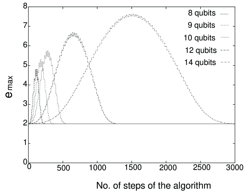
Figure 1: The maximum eigenvalue $e_{\rm max}$ of the VCM of quantum states appearing in Grover’s quantum search algorithm for $L=8,9,10,12$ and $14$ when $x_{1}=19,388,799,1332$ and $9875$, respectively, as functions of the number of step of the algorithm. The horizontal line represents $e_{\rm max}$ for product states, $e_{\rm max}=2$.

Figure 2 is a magnification from the $1$st step to the $40$th step for $L=8$, whereas Fig. 3 shows a magnification from the $1005$th step to the $1155$th step for $L=14$.

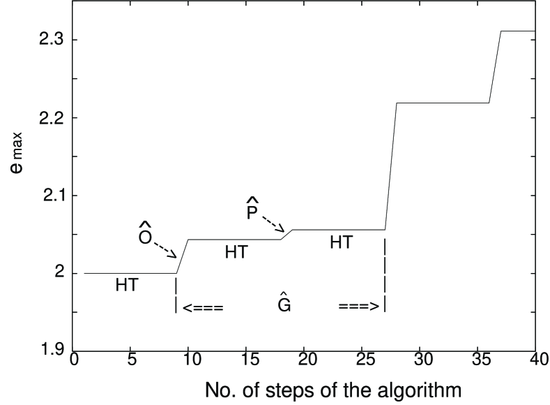
Figure 2: Magnification of Fig. 1, from the $1$st step to the $40$th step for $L=8$. Here, $\hat{O}$ and $\hat{P}$ represent the oracle operation and conditional phase shift, respectively, in a single Grover iteration $\hat{G}$.

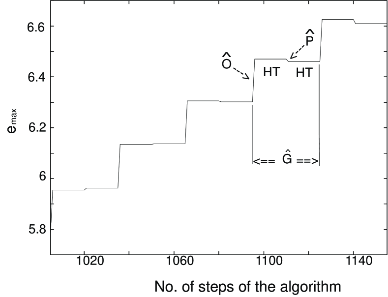
Figure 3: Magnification of Fig. 1, from the $1005$th step to the $1155$th step for $L=14$. Here, $\hat{O}$ and $\hat{P}$ represent the oracle operation and conditional phase shift, respectively, in a single Grover iteration $\hat{G}$.

It is seen that $e_{\rm max}=2.00$ for all states from $|\psi_{\rm init}\rangle$ to $|\psi_{0}\rangle$, i.e., during the initial HT (from the $1$st step to the $8$th step in Fig. 2, denoted as ‘HT’). This is because all these states are product states, for which we can easily show that $e_{\rm max}=2$ (Appendix H). When the stage of Grover iterations begins, $e_{\rm max}$ grows gradually, as seen from Figs. 1 and 2. In each Grover iteration, Figs. 2 and 3 show that $e_{\rm max}$ changes when the oracle operator $\hat{O}$ is operated, whereas it remains constant during the subsequent HT. Then, it changes again when $\hat{P}$ is operated, whereas it remains constant again during the subsequent HT. As the Grover iterations are repeated, $e_{\rm max}$ (hence, quantum correlation) continues to increase as a whole, until it becomes maximum after about $R(L)/2$ applications of $\hat{G}$. Further applications of $\hat{G}$ reduce $e_{\rm max}$, as seen from Fig. 1, toward $e_{\rm max}\simeq 2.00$ for $|\psi_{R(L)}\rangle$, which is approximately a product state as seen from eq. (58).

These results indicate that our construction of the family of states, given by eqs. (45) and (46), is reasonable. Although we have already shown in §4 that $p=2$ for such a family, it is instructive to plot $e_{\rm max}(L,\nu)$ of $|\psi_{k_{*}}(L,\nu)\rangle$ as a function of $L$ when the solution $x_{1}$ is randomly chosen (i.e., an instance $\nu$ is randomly chosen) for each $L$. Figure 4 shows $e_{\rm max}$’s of $|\psi_{\lceil R/2\rceil}\rangle$, $|\psi_{\lceil R/3\rceil}\rangle$ and $|\psi_{\lceil R/4\rceil}\rangle$ as functions of $L$ for such a randomly chosen $x_{1}$. [We have confirmed that almost identical curves are obtained for other choices of $x_{1}$ as well.] Since $e_{\rm max}$’s tend to be proportional to $L$ for large $L$, we can confirm that $p=p_{e}=2$.

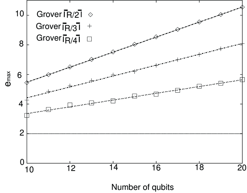
Figure 4: $e_{\rm max}$’s of $|\psi_{\lceil R/2\rceil}\rangle$ (diamonds), $|\psi_{\lceil R/3\rceil}\rangle$ (crosses) and $|\psi_{\lceil R/4\rceil}\rangle$ (squares) as functions of $L$. They all show that $p=p_{e}=2$. The dotted lines are guides to the eyes, whereas the horizontal line represents $e_{\rm max}$ for product states, $e_{\rm max}=2$.

5.3 Results of simulation for $M=2$

When $M=2$, the result in §4.5 indicates that $p=2$ for most states in the Grover iteration processes whereas $p$ of the final state depends on the nature of the solutions. Figure 5 shows this clearly, where we have plotted the evolution of $e_{\rm max}$ in two cases, i.e., $p=2$ (profile 1) and $p=1$ (profile 2) for the final state. For $|\psi_{\lceil R/2\rceil}\rangle$, $|\psi_{\lceil R/3\rceil}\rangle$ and $|\psi_{\lceil R/4\rceil}\rangle$, on the other hand, we obtain results similar to those in Fig. 4 in both cases. Hence, $p=2$ for these states. This result visualizes how our extended conjecture holds when $M\geq 2$.

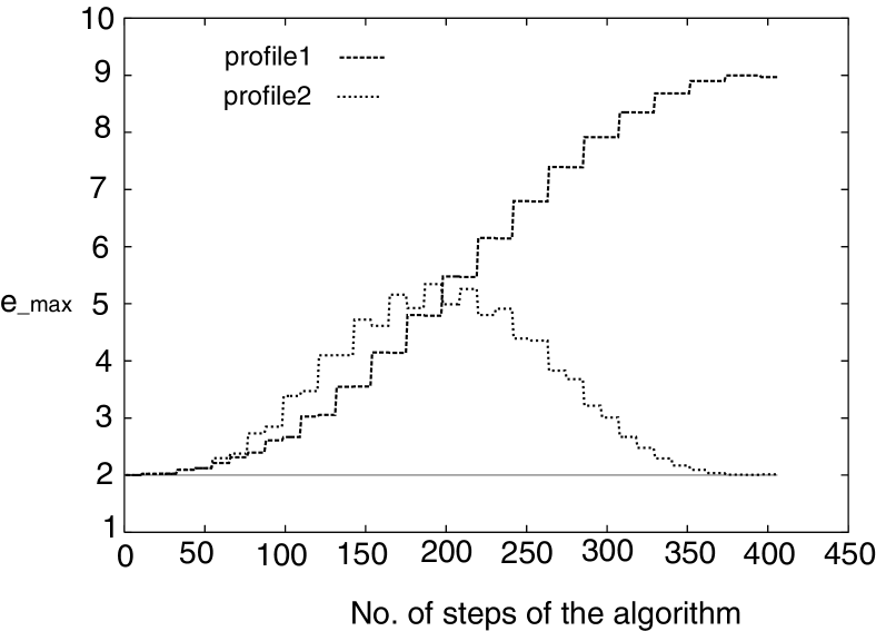
Figure 5: The maximum eigenvalue $e_{\rm max}$ of the VCM of quantum states appearing in Grover’s quantum search algorithm for $L=10$ and $M=2$, when $x_{1}=2,x_{2}=1023$ (profile 1) and when $x_{1}=511,x_{2}=512$ (profile 2), as functions of the number of steps of the algorithm. The horizontal line represents the value of $e_{\rm max}$ for product states, $e_{\rm max}=2$.

6 Discussion and Summary

We have studied the conjecture that the superposition of macroscopically distinct states is necessary for the significant speedup of quantum computers over classical computers. This conjecture was previously supported for a circuit-based quantum computer performing Shor’s factoring algorithm. To treat general algorithms and models, we have generalized the indices $p$ and $q$, which detect the superposition of macroscopically distinct states. We then generalize the conjecture in such a way that it is unambiguously applicable to general models if a quantum algorithm achieves an exponential speedup. We further extend the conjecture to the speedup achieved by Grover’s quantum search algorithm. This extended conjecture is proved to be correct for Grover’s algorithm. Since Grover’s and Shor’s algorithms are representative algorithms for unstructured and structured problems, respectively, the present results and the results of ref. US04 strongly support the conjecture. To see details, we have also presented, by numerical simulation, how quantum correlation evolves and how the superposition of macroscopically distinct states develops as the computation proceeds.

Jozsa and Linden previously showed that entanglement over a cluster whose size is larger than $O(1)$ is necessary for exponential speedup [18]. For $p=2$, on the other hand, entanglement over a cluster whose size is larger than $O(L)$ is necessary [11, 12]. The present conjecture imposes a stronger condition in this sense.

Moreover, Vidal showed that a necessary condition for exponential speedup is that the amount of the bipartite entanglement between one part and the rest of the qubits increases with $L$ [19]. The bipartite entanglement studied by him is totally different from the entanglement associated with the superposition of macroscopically distinct states. Therefore, the simultaneous requirement (for speedup over classical computations) of Vidal’s condition and the present conjecture is much stronger than the requirement of either one of them. That is, for quantum speedup both the superposition of macroscopically distinct states and sufficient bipartite entanglement are necessary.

It is also interesting to explore the relation between our results and the problem of time-optimal quantum evolution [40, 41]. In the latter case, the optimal evolution requires a large fluctuation of the Hamiltonian operator, while in the former, fast quantum computations require states with large fluctuations of additive operators. This suggests a possible relation between quantum speedup and optimal evolution [41].

Appendix A $p=2$ implies superposition of macroscopically distinct states

In this appendix, we explain why $p=2$ implies the superposition of macroscopically distinct states, assuming for simplicity spatially homogeneous states.

Two states are macroscopically distinct if there is a macroscopic quantity whose expectation value is macroscopically distinct between them. There are many quantities that are known as macroscopic quantities, including entropy, temperature, and pressure. Among them, ‘additive mechanical variables’, such as the total energy and the total magnetic moment, can be expressed by additive operators, as eq. (4). [In contrast, ‘genuine thermodynamical variables’, such as the entropy and temperature, cannot be expressed by additive operators.]

Let $L$ be the size of a macroscopic system. In macroscopic physics such as thermodynamics, the values of additive mechanical variables scale as $\propto L$ with increasing $L$. Therefore, the difference of an additive mechanical variable between two states is neglected if the difference is only $o(L)$ because the ratio of the difference to typical values vanishes in the macroscopic limit $L\to\infty$. In other words, two values of additive mechanical variables are macroscopically distinct only when their difference scales as $\propto L$. If one treats this macroscopic system by quantum theory, eigenvalues of an additive operator $\hat{A}(L)$ scale as $\propto L$. Therefore, two eigenvalues or expectation values are macroscopically distinct only when their difference scales as $\propto L$.

Consider a state $|\psi(L)\rangle$ in a family of states of various values of $L$, $\{|\psi(L)\rangle\}_{L}$. Let $|A,\mu;L\rangle$ be an eigenvector of $\hat{A}(L)$ corresponding to an eigenvalue $A$, where $\mu$ labels degenerate eigenvectors. If $|\psi(L)\rangle$ is not a superposition of states with macroscopically distinct values of $A$, i.e., if it is just a superposition of $|A,\mu;L\rangle$’s with macroscopically nondistinct values of $A$ ($+$ terms that vanish as $L\to\infty$), then $|\langle A,\mu;L|\psi(L)\rangle|^{2}$ takes nonvanishing (or significant) values only for $A$ such that $\left|A-\langle\psi(L)|\hat{A}(L)|\psi(L)\rangle\right|=o(L)$. In this case, $\langle\psi(L)|\Delta\hat{A}(L)^{\dagger}\Delta\hat{A}(L)|\psi(L)\rangle=o(L^{2})$. Hence, by contradiction, if $\langle\psi(L)|\Delta\hat{A}(L)^{\dagger}\Delta\hat{A}(L)|\psi(L)\rangle\neq o(L^{2})$ then $|\psi(L)\rangle$ is a superposition of states with macroscopically distinct values of $A$. Therefore, a sufficient condition for $|\psi(L)\rangle$ being a superposition of macroscopically distinct states is that there exists an additive operator(s) $\hat{A}(L)$ (among many additive operators) such that $\langle\psi(L)|\Delta\hat{A}(L)^{\dagger}\Delta\hat{A}(L)|\psi(L)\rangle=\Theta(L^{2})$. [The asymptotic notation such as $\Theta$ is summarized in Appendix C.] This condition is simply expressed as

$$\max_{\hat{A}(L)}\langle\psi(L)|\Delta\hat{A}(L)^{\dagger}\Delta\hat{A}(L)|\psi(L)\rangle=\Theta(L^{2}).$$ (61)

By definition, this means that $\{|\psi(L)\rangle\}_{L}$ has $p=2$. Therefore, $p=2$ implies the superposition of macroscopically distinct states.

For the argument in the present paper, we use this sufficient condition. A state with $p<2$ may or may not be a superposition of macroscopically distinct states, depending on one’s interest. However, such states with $p<2$ are irrelevant to conclusions of the present paper.

Note that, in the above argument, we have never assumed that only two macroscopically distinct states are superposed to form $|\psi(L)\rangle$ with $p=2$. Therefore, $|\psi(L)\rangle$ with $p=2$ is a superposition of two or more macroscopically distinct states.

To illustrate how $p$ is useful, we give a few simple examples.

For the GHZ or ‘cat’ state, $|\psi_{\rm cat}(L)\rangle\equiv(|00\cdots 0\rangle+|11\cdots 1\rangle)/\sqrt{2}$, a heuristic discussion would be sufficient to determine that it is a superposition of macroscopically distinct states, because it is simply a superposition of two macroscopically distinct states and their coefficients do not vanish as $L\to\infty$.

On the other hand, let us consider the following state;

$${1\over\sqrt{L-1}}\big{(}|100\cdots 00\rangle+|110\cdots 00\rangle+\cdots+|111\cdots 10\rangle\big{)}$$

$$\quad={1\over\sqrt{L-1}}\sum_{j=1}^{L-1}|j;j+1\rangle,$$ (62)

where $|j;j+1\rangle$ is the state that has a ‘domain wall’ between sites $j$ and $j+1$. In this sum, each state differs from the preceeding state only in a single qubit, and the weight of each state vanishes in the $L\to 0$ limit. For such a state, heuristic discussions will be ambiguous. Even for such a state, by using the index $p$, we can easily show that it is a superposition of macroscopically distinct states because it has $p=2$.

By contrast, the ‘W state’ $\left(|100\cdots 0\rangle+|010\cdots 0\rangle+\cdots+|000\cdots 1\rangle\right)/\sqrt{L}$ has $p=1$, hence one cannot say that it is a superposition of macroscopically distinct states [11, 12]. This is reasonable because the W state corresponds to normal states in condensed-matter physics, such as a Frenkel exciton excited in an insulating solid [22], which can be created easily in experiments. In contrast, states with $p=2$ are extremely abnormal in view of many-body physics, as discussed in §2.3 and ref. SM02.

Regarding the index $q$ for mixed states, see ref. SM05 for its physical meaning and several examples.

Appendix B On the restriction that $\|\hat{a}(l)\|=1$

Suppose that $\hat{A}=\sum_{l}\hat{a}(l)$ is an additive operator. In the present paper, we have required that $\|\hat{a}(l)\|=1$. To understand technical details about this, the following examples would be helpful.

• The operator $\hat{A}^{\prime\prime}_{1}\equiv\sum_{l}\hat{a}(l)/2$ is not an additive operator according to the present definition, because the norm of the local operators is not unity. However, by simply multiplying $\hat{A}^{\prime\prime}_{1}$ by $2$, we can obtain an additive operator $\hat{A}_{1}\equiv 2\hat{A}^{\prime\prime}_{1}$ ($=\hat{A}$). The fluctuations of $\hat{A}_{1}$ and $\hat{A}^{\prime\prime}_{1}$ differ only by a constant factor.

• The operator $\hat{A}^{\prime\prime}_{2}\equiv\sum_{l={\rm odd}}\hat{a}(l)$ is not an additive operator according to the present definition, because the norm of the local operators for even $l$ vanishes. However, this operator has the same fluctuation as the additive operator $\hat{A}_{2}\equiv\sum_{l={\rm odd}}\hat{a}(l)+\sum_{l={\rm even}}\hat{1}(l)$.

• The operator $\hat{A}^{\prime\prime}_{3}\equiv\sum_{l}\left(1+{(-1)^{l}\over 2}\right)\hat{a}(l)$ is not an additive operator according to the present definition. However, there always exist real numbers $\alpha,\beta(l)$ such that $\hat{a}_{3}(l)\equiv\alpha\left(1+{(-1)^{l}\over 2}\right)\hat{a}(l)+\beta(l)\hat{1}(l)$ has a unit norm for every $l$. Then, $\hat{A}_{3}\equiv\sum_{l}\hat{a}_{3}(l)$ is an additive operator, and the fluctuations of $\hat{A}_{3}$ and $\hat{A}^{\prime\prime}_{3}$ differ only by a constant factor.

Therefore, operators like $\hat{A}^{\prime\prime}_{1},\hat{A}^{\prime\prime}_{2}$ and $\hat{A}^{\prime\prime}_{3}$ are essentially included (as $\hat{A}_{1},\hat{A}_{2}$ and $\hat{A}_{3}$, respectively) when taking $\max_{\hat{A}(L)}$ in eq. (5).

The point is that one can modify $\hat{A}^{\prime\prime}_{1},\hat{A}^{\prime\prime}_{2}$ and $\hat{A}^{\prime\prime}_{3}$ in such a way that the fluctuations of the modified operators $\hat{A}_{1},\hat{A}_{2}$ and $\hat{A}_{3}$ (which are additive operators), respectively, have the same order of magnitude as those of $\hat{A}^{\prime\prime}_{1},\hat{A}^{\prime\prime}_{2}$ and $\hat{A}^{\prime\prime}_{3}$. Note that this modification is not unique. For example, from $\hat{A}^{\prime\prime}_{1}$, one can also construct the additive operator $2\hat{A}^{\prime\prime}_{1}-\hat{a}(1)+\hat{1}(1)=\hat{1}(1)+\sum_{l\geq 2}\hat{a}(l)$, which has the same order of fluctuation as $\hat{A}_{1}$. This nonuniqueness does not cause any difficulty because $p$ and $q$ are defined by the order of magnitude of fluctuations.

Appendix C Asymptotic notation

Let $f(L)$ and $g(L)$ be non-negative functions of a positive variable $L$. Following ref. NC, we use the following asymptotic notation:

$$f(L)=O(g(L)) \Leftrightarrow f(L)\leq Kg(L),$$ (63)

$$f(L)=\Omega(g(L)) \Leftrightarrow Jg(L)\leq f(L),$$ (64)

$$f(L)=\Theta(g(L)) \Leftrightarrow Jg(L)\leq f(L)\leq Kg(L),$$ (65)

as $L\to\infty$, where $J$ and $K$ are some positive constants.

Let $f_{\nu}(L)$’s be non-negative functions, which are labeled by an index $\nu$, of a positive variable $L$. We consider a family that consists of these functions, i.e., a family of real values, $\{f_{\nu}(L)\}_{L,\nu}$. Assuming that the number of possible values of $\nu$ increases to infinity as $L\to\infty$, we use the following asymptotic notation:

$$f_{\nu}(L)=\overline{O}(g(L)) \Leftrightarrow f_{\nu}(L)=O(g(L))$$ (66)

$$\quad\mbox{ for almost every $\nu$},$$

$$f_{\nu}(L)=\overline{\Omega}(g(L)) \Leftrightarrow f_{\nu}(L)=\Omega(g(L))$$ (67)

$$\quad\mbox{ for almost every $\nu$},$$

$$f_{\nu}(L)=\overline{\Theta}(g(L)) \Leftrightarrow f_{\nu}(L)=\Theta(g(L))$$ (68)

$$\quad\mbox{ for almost every $\nu$}.$$

For example, if $\nu=1,2,\ldots,2^{L}$ for each $L$ and $f_{\nu}(L)=L^{3}(1+\sin L)(1/L-1/L^{\nu})$, then $f_{\nu}(L)=\overline{\Theta}(L^{2})$, whereas it is not $\Theta(L^{2})$.

Appendix D Range of $p$

In this appendix, we show that $1\leq p\leq 2$. As the operator norm $\|\hat{a}\|$, we employ $\|\hat{a}\|_{E}$, defined by eq. (2), in this Appendix. Since $\left\langle\left(\Delta\hat{A}(L)\right)^{2}\right\rangle_{L\nu}\leq\left\langle\hat{A}(L)^{2}\right\rangle_{L\nu}\leq L^{2},$ we find that $p\leq 2$. To prove that $p\geq 1$, we use the following Lemma;
Lemma: For any state, which can be a mixed state, there always exists a local operator $\hat{a}_{*}(l)$ that satisfies

$$\|\hat{a}_{*}(l)\|_{E}=1\ \mbox{and}\ \langle\Delta\hat{a}_{*}(l)^{\dagger}\Delta\hat{a}_{*}(l)\rangle=1,$$ (69)

Proof: For a given state $\hat{\rho}(L)$, its local density operator $\hat{\rho}_{l}\equiv{\rm Tr}_{l^{\prime}(\neq l)}\hat{\rho}(L)$ can be diagonalized as

$$\hat{\rho}_{l}=\sum_{j=1}^{d}w_{j}(l)|j,l\rangle\langle j,l|,\quad\sum_{j=1}^{d}w_{j}(l)=1,$$ (70)

where $\{|j,l\rangle\}_{j}$ is a complete orthonormal set of site $l$. Take

$$\hat{a}_{*}(l)=\sum_{j={\rm odd}}\left(|j,l\rangle\langle j+1,l|+h.c.\right)$$ (71)

where $\langle d+1,l|\equiv\langle 1,l|$. This is a Hermitian local operator with $\|\hat{a}_{*}(l)\|_{E}=1$. Since ${\rm Tr}\left[\hat{\rho}(L)\hat{a}_{*}(l)\right]=0$ and

$$\hat{a}_{*}(l)^{\dagger}\hat{a}_{*}(l)=\sum_{j=1}^{d}|j,l\rangle\langle j,l|=\hat{1}(l),$$ (72)

we find that $\langle\Delta\hat{a}_{*}(l)^{\dagger}\Delta\hat{a}_{*}(l)\rangle=1$. $\blacksquare$

Using this Lemma, we now show the following theorem, from which it is evident that $p\geq 1$.
Theorem: For any state, which can be a mixed state, there always exists an additive operator that satisfies

$$\langle\Delta\hat{A}(L)^{\dagger}\Delta\hat{A}(L)\rangle\geq L.$$ (73)

Proof: We use the induction method. We define

$$\hat{A}(k)\equiv\sum_{l=1}^{k}\hat{a}(l)\quad(\|\hat{a}(l)\|=1),$$ (74)

for $1\leq k\leq L$. When $k=1$, the above Lemma shows that there exists $\hat{A}(1)$ such that $\langle\Delta\hat{A}(1)^{\dagger}\Delta\hat{A}(1)\rangle\geq 1$. Now, assume that there exists $\hat{A}(k)$ such that $\langle\Delta\hat{A}(k)^{\dagger}\Delta\hat{A}(k)\rangle\geq 1$. From the above Lemma, there exists a local operator $\hat{a}_{*}(k+1)$ on site $k+1$ such that $\|\hat{a}_{*}(k+1)\|=1$ and $\langle\Delta\hat{a}_{*}(k+1)^{\dagger}\Delta\hat{a}_{*}(k+1)\rangle=1.$ So, construct $\hat{A}(k+1)$ as

$$\hat{A}(k+1)=\hat{A}(k)+\hat{a}_{*}(k+1).$$ (75)

Then,

$$\langle\Delta\hat{A}(k+1)^{\dagger}\Delta\hat{A}(k+1)\rangle$$

$$\quad=\langle\Delta\hat{A}(k)^{\dagger}\Delta\hat{A}(k)\rangle$$

$$\qquad+\left\{\langle\Delta\hat{A}(k)^{\dagger}\Delta\hat{a}_{*}(k+1)\rangle+c.c.\right\}+1.$$ (76)

Therefore, if $\left\{\langle\Delta\hat{A}(k)^{\dagger}\Delta\hat{a}_{*}(k+1)\rangle+c.c.\right\}\geq 0$, then $\langle\Delta\hat{A}(k+1)^{\dagger}\Delta\hat{A}(k+1)\rangle\geq k+1$. If, on the other hand, $\left\{\langle\Delta\hat{A}(k)^{\dagger}\Delta\hat{a}_{*}(k+1)\rangle+c.c.\right\}<0$, then reconstruct $\hat{A}(k+1)$ as

$$\hat{A}(k+1)=\hat{A}(k)-\hat{a}_{*}(k+1).$$ (77)

This gives $\langle\Delta\hat{A}(k+1)^{\dagger}\Delta\hat{A}(k+1)\rangle\geq k+1$. $\blacksquare$

Appendix E Approach of a pure state with $p=2$ to a mixed state as $L\to\infty$

It was proved rigorously that any pure state with $p=2$ in a finite system of size $L$ does not approach pure states in an infinite system as $L\to\infty$ [11]. Although this might sound strange to the reader who is not familiar with the quantum theory of infinite systems [31], its physics can be understood as follows.

In the quantum theory of finite systems, all possible representations are equivalent (unitary equivalence). In the quantum theory of infinite systems, by contrast, many representations that are not equivalent to each other can exist [31]. Among two or more inequivalent representations, we have to choose one that is suitable for describing the physical states of interest [31]. This makes the quantum theory of infinite systems very different from that of finite systems. The above strange fact comes from this great difference.

As the simplest example, consider a cat state $|\psi(L)\rangle\equiv(|00\cdots 0\rangle+|11\cdots 1\rangle)/\sqrt{2}$ of size $L$. If $L$ is finite, there exist observables that have nonvanishing matrix elements between $|00\cdots 0\rangle$ and $|11\cdots 1\rangle$. The expectation values of such observables discriminate between the pure state $|\psi(L)\rangle$ and the mixed state $\rho(L)\equiv(|00\cdots 0\rangle\langle 00\cdots 0|+|11\cdots 1\rangle\langle 11\cdots 1|)/2$. If we take the $L\to\infty$ limit, however, the quantum theory of infinite systems requires that every observables should be a function of field operators within a finite region in an infinite space [31]. As a result, there are no observables that have nonvanishing matrix elements between the $L\to\infty$ limits of $|00\cdots 0\rangle$ and $|11\cdots 1\rangle$. This implies that $\lim_{L\to\infty}|\psi(L)\rangle$ is not a pure state. Here, the rigorous definition of pure states in ref. Haag is used instead of the (over)simplified definition $\hat{\rho}^{2}=\hat{\rho}$, because the latter can be used only for (an irreducible representation for) finite systems.

More mathematically speaking, if $|\psi(L)\rangle$ has $p=2$ then $\lim_{L\to\infty}|\psi(L)\rangle$ is not a vector state of an irreducible representation. For details, see ref. SM02 and references cited therein.

Appendix F Equivalence of $p_{e}=2$ and $p=2$

In this appendix, we show that if $p_{e}=2$ then $p=2$ and vice versa. For simplicity, we will omit ‘$\nu$’ and ‘$(L)$’, i.e., we will abbreviate $\hat{A}^{\prime}(L),|\psi_{\nu}(L)\rangle,C_{\nu}(L)$ and so on to $\hat{A}^{\prime},|\psi\rangle,C$ and so on, respectively. We first note that

$$\left\|\Delta\hat{A}^{\prime}|\psi\rangle\right\|^{2} = \left\|\sum_{l=1}^{L}\sum_{\alpha=1}^{D}c^{\prime}_{l\alpha}\Delta\hat{b}_{\alpha}(l)|\psi\rangle\right\|^{2}$$ (78)

$$\leq \left[\sum_{l=1}^{L}\sum_{\alpha=1}^{D}\left|c^{\prime}_{l\alpha}\right|^{2}\right]\left[\sum_{l=1}^{L}\sum_{\alpha=1}^{D}\left\|\Delta\hat{b}_{\alpha}(l)|\psi\rangle\right\|^{2}\right]$$

$$\leq L\overline{O}(L),$$

from which $p_{e}\leq 2$. Here, we have used the inequality $\sum_{k}\left|\sum_{j}x_{j}y_{jk}\right|^{2}\leq\sum_{k}\sum_{j}\left|x_{j}\right|^{2}\sum_{j^{\prime}}\left|y_{j^{\prime}k}\right|^{2}=\sum_{j}\left|x_{j}\right|^{2}\sum_{j^{\prime}}\sum_{k}\left|y_{j^{\prime}k}\right|^{2}$, which holds for arbitrary complex numbers $x_{j},y_{jk}$. On the other hand, it is clear from the definitions that

$$p\leq p_{e}.$$ (79)

Therefore, if $p=2$ then $p_{e}=2$.

To show the inverse, we assume that $p_{e}=2$, i.e., eq. (22) holds. Without loss of generality, we also assume that $\max_{l,\alpha}\left|c^{\prime}_{l\alpha\,{\rm max}}\right|^{2}=\left|c^{\prime}_{11\,{\rm max}}\right|^{2}.$ It is clear from eq. (20) that

$$\left|c^{\prime}_{11\,{\rm max}}\right|^{2}\leq L.$$ (80)

Our purpose is to show that

$$\left|c^{\prime}_{11\,{\rm max}}\right|^{2}=\overline{O}(L^{0}),$$ (81)

because it yields $C=\overline{O}(L^{0})$, which gives eq. (25) (implying $p=2$). Equation (22) can be rewritten as

$$\sum_{\alpha,\alpha^{\prime}=1}^{D}c^{\prime\,*}_{1\alpha\,{\rm max}}c^{\prime}_{1\alpha^{\prime}\,{\rm max}}V_{1\alpha,1\alpha^{\prime}}$$

$$\quad+\left(\sum_{l=2}^{L}\sum_{\alpha,\alpha^{\prime}=1}^{D}c^{\prime\,*}_{l\alpha\,{\rm max}}c^{\prime}_{1\alpha^{\prime}\,{\rm max}}V_{l\alpha,1\alpha^{\prime}}+c.c.\right)$$

$$\quad+\sum_{l,l^{\prime}=2}^{L}\sum_{\alpha,\alpha^{\prime}=1}^{D}c^{\prime\,*}_{l\alpha\,{\rm max}}c^{\prime}_{l^{\prime}\alpha^{\prime}\,{\rm max}}V_{l\alpha,l^{\prime}\alpha^{\prime}}=\overline{O}(L^{2}).$$

(82)

The first term is positive (because the VCM is a non-negative Hermitian matrix) and $\leq\overline{O}(L)$. The second term is estimated as

$$\left|\sum_{l=2}^{L}\sum_{\alpha,\alpha^{\prime}=1}^{D}c^{\prime\,*}_{l\alpha\,{\rm max}}c^{\prime}_{1\alpha^{\prime}\,{\rm max}}V_{l\alpha,1\alpha^{\prime}}\right|$$

$$\quad\leq D|c^{\prime}_{11\,{\rm max}}|\left|\sum_{l=2}^{L}\sum_{\alpha=1}^{D}c^{\prime\,*}_{l\alpha\,{\rm max}}\right|\max_{l,\alpha,\alpha^{\prime}}\left|V_{l\alpha,1\alpha^{\prime}}\right|$$

$$\quad\leq D|c^{\prime}_{11\,{\rm max}}|\sqrt{D(L-1)}\sqrt{L}\max_{l,\alpha,\alpha^{\prime}}\left|V_{l\alpha,1\alpha^{\prime}}\right|$$

$$\quad\leq|c^{\prime}_{11\,{\rm max}}|\overline{O}(L)\leq\overline{O}(L^{3/2}),$$ (83)

where we have used inequality (80) and $|\vec{x}\cdot\vec{1}|\leq|\vec{x}||\vec{1}|=n|\vec{x}|$, which holds for an arbitrary $n$-dimensional vector $\vec{x}$. Therefore, the third term of eq. (82) should be

$$\sum_{l,l^{\prime}=2}^{L}\sum_{\alpha,\alpha^{\prime}=1}^{D}c^{\prime\,*}_{l\alpha\,{\rm max}}c^{\prime}_{l^{\prime}\alpha^{\prime}\,{\rm max}}V_{l\alpha,l^{\prime}\alpha^{\prime}}=\overline{O}(L^{2}).$$ (84)

On the other hand, let

$$c^{\prime}_{l\alpha}\equiv{1\over\sqrt{1-\sum_{\alpha=1}^{D}|c^{\prime}_{l\alpha\,{\rm max}}|^{2}/L}}c^{\prime}_{l\alpha\,{\rm max}},$$ (85)

then the following operator, which does not involve an operator on site $1$, takes the form of eq. (15):

$$\Delta\hat{A}^{\prime}\equiv\sum_{l=2}^{L}\sum_{\alpha=1}^{D}c^{\prime}_{l\alpha}\Delta\hat{b}_{\alpha}(l).$$ (86)

We therefore have, using eqs. (83) and (84),

$$0 \leq \langle\Delta\hat{A}^{\prime\nu\dagger}_{\rm max}\Delta\hat{A}^{\prime\nu}_{\rm max}\rangle_{L\nu}-\langle\Delta\hat{A}^{\prime\nu\dagger}\Delta\hat{A}^{\prime\nu}\rangle_{L\nu}$$

$$\leq \sum_{\alpha,\alpha^{\prime}=1}^{D}c^{\prime\,*}_{1\alpha\,{\rm max}}c^{\prime}_{1\alpha^{\prime}\,{\rm max}}V_{1\alpha,1\alpha^{\prime}}$$

$$+\left(\sum_{l=2}^{L}\sum_{\alpha,\alpha^{\prime}=1}^{D}c^{\prime\,*}_{l\alpha\,{\rm max}}c^{\prime}_{1\alpha^{\prime}\,{\rm max}}V_{l\alpha,1\alpha^{\prime}}+c.c.\right)$$

$$-{|c^{\prime}_{11\,{\rm max}}|^{2}\over L}\sum_{l,l^{\prime}=2}^{L}\sum_{\alpha,\alpha^{\prime}=1}^{D}c^{\prime\,*}_{l\alpha\,{\rm max}}c^{\prime}_{l^{\prime}\alpha^{\prime}\,{\rm max}}V_{l\alpha,l^{\prime}\alpha^{\prime}}$$

$$\leq |c^{\prime}_{11\,{\rm max}}|^{2}\overline{O}(L^{0})+|c^{\prime}_{11\,{\rm max}}|\overline{O}(L)-{|c^{\prime}_{11\,{\rm max}}|^{2}\over L}\overline{O}(L^{2})$$

$$\leq |c^{\prime}_{11\,{\rm max}}|\left[|c^{\prime}_{11\,{\rm max}}|\overline{O}(L^{0})+\overline{O}(L)-|c^{\prime}_{11\,{\rm max}}|\overline{O}(L)\right].$$

Therefore, eq. (81) should be satisfied because, otherwise, the last line would become negative in contradiction with the first line.

For a family of homogeneous states, in particular, $p=p_{e}$ for every value of $p$, because in this case the VCM has the translational invariance, and thus an eigenvector corresponding to $e_{\rm max}$ is also translational-invariant. [Even when $e_{\rm max}$ is a degenerate eigenvalue, one can construct a translational-invariant eigenvector by taking a linear combination of eigenvectors corresponding to $e_{\rm max}$.] From eq. (20), this means $C=\overline{O}(L^{0})$ for the additive operator that is composed of such an eigenvector, and thus $p\geq p_{e}$. From inequality (79), this yields $p=p_{e}$.

Appendix G Proof of $\langle\beta|\hat{M}_{x}|\beta\rangle=KL$ for $M=2^{mL}$

In this appendix, we prove $\langle\beta|\hat{M}_{x}|\beta\rangle\leq KL$ $(0<K<1)$ for $M=2^{mL}$ where $K$ is independent of $L$. We use the following lemma:
Lemma: There exists a real number $K$ independent of $L$ such that $2^{(1-m)}(1-K)^{1-K}K^{K}>1$ and $\frac{1}{2}<K<1$.
Proof: Consider the following function:

$$f(k) = (1-m)\log 2+k\log k$$ (88)

$$+(1-k)\log(1-k)\ \ (\frac{1}{2}\leq k<1),$$

where $0<m<1$. Since $f(\frac{1}{2})=-m\log 2<0$, $f(k)\rightarrow(1-m)\log 2>0\ (k\rightarrow 1)$, and the function $f(k)$ is continuous at $\frac{1}{2}\leq k<1$, we can apply the intermediate-value theorem, therefore, there exists a real number $K$ such that $f(K)>0$ and $1/2<K<1$. $\blacksquare$

Now, we prove $\langle\beta|\hat{M}_{x}|\beta\rangle=kL\ (0<k<1)$ for $M=2^{mL}$. Let $P(M_{x}=-L+2j)$ be the probability of getting a value $-L+2j$ when one measures $\hat{M}_{x}$, where $j=0,1,\cdots,L$. It is represented as

$$P(M_{x}=-L+2j) = \sum_{\nu}\big{|}\langle M_{x}=-L+2j,\nu|\beta\rangle\big{|}^{2}$$

$$\leq {L\choose j}\max_{\nu}[\ \big{|}\langle M_{x}=-L+2j,\nu|\beta\rangle\big{|}^{2}\ ],$$

where $|M_{x}=L-j,\nu\rangle$ is an eigenstate of $\hat{M}_{x}$, and $\nu=1,2,\cdots,{L\choose j}$ labels degenerate eigenstates. Since

$$\big{|}\langle M_{x}=-L+2j,\nu|\beta\rangle\big{|} \leq \frac{1}{\sqrt{M}}\sum_{n=1}^{M}\big{|}\langle M_{x}=-L+2j,\nu|x_{n}\rangle\big{|}$$ (90)

$$\leq \sqrt{\frac{M}{2^{L}}},$$

we have, using Stirling’s formula $n!\sim\sqrt{2\pi n}(n/e)^{n}$,

$$P(M_{x}=-L+2j)$$

$$\leq{L\choose j}\frac{M}{2^{L}}$$

$$\sim\frac{1}{\sqrt{2\pi j(1-\frac{j}{L})}\{2^{(1-m)}(1-\frac{j}{L})^{1-\frac{j}{L}}(\frac{j}{L})^{\frac{j}{L}}\}^{L}}.$$ (91)

From the above Lemma, there exists a real number $K$ independent of $L$ such that $2^{(1-m)}(1-K)^{1-K}K^{K}>1$ and $\frac{1}{2}<K<1$. Hence,

$$L^{n}P(M_{x}=-L+2j)\rightarrow 0\ \ (KL\leq j\leq L)\ \text{ as }L\rightarrow\infty,$$ (92)

where $n$ is independent of $L$. This yields

$$\langle\beta|\hat{M}_{x}|\beta\rangle\to\sum_{j=0}^{KL-1}(-L+2j)P(M_{x}=-L+2j)$$ (93)

as $L\rightarrow\infty$, from which we conclude that $\langle\beta|\hat{M}_{x}|\beta\rangle\leq KL$ for large $L$. $\blacksquare$

Appendix H Maximum eigenvalue of the VCM for product states

In this appendix, we show that $e_{\rm max}=2$ for a product state, $|\psi\rangle=\bigotimes_{l=1}^{L}|\phi_{l}\rangle_{l},$ where $|\phi_{l}\rangle_{l}$ denotes a state of the qubit at site $l$ ($=1,2,\cdots,L$). The VCM of such a state is block-diagonal:

$$\left(\begin{array}[]{ccccc}\bm{V}_{1}&0&\cdots&\cdots&0\\ 0&\bm{V}_{2}&0&\cdots&\cdots\\ \vdots&0&\bm{V}_{3}&0&\cdots\\ \vdots&\vdots&&\cdots&\cdots\\ 0&\cdots&\cdots&0&\bm{V}_{L}\end{array}\right),$$ (94)

where $\bm{V}_{l}$ is a $3\times 3$ matrix whose $\alpha\beta$ element ($\alpha,\beta=x,y,z$) is given by

$$(V_{l})_{\alpha\beta}=\langle\phi_{l}|\hat{\sigma}_{\alpha}(l)\hat{\sigma}_{\beta}(l)|\phi_{l}\rangle-\langle\phi_{l}|\hat{\sigma}_{\alpha}(l)|\phi_{l}\rangle\langle\phi_{l}|\hat{\sigma}_{\beta}(l)|\phi_{l}\rangle.$$ (95)

Therefore, $e_{\rm max}$ is given by the maximum one among the eigenvalues of $\bm{V}_{l}$’s. By a unitary transformation of this $3\times 3$ matrix such that $|\phi_{l}\rangle$ becomes an eigenstate of the transformed $\hat{\sigma}_{z}(l)$, we can transform $\bm{V}_{l}$ into

$$\bm{V}_{l}=\left(\begin{array}[]{ccc}1&i&0\\ -i&1&0\\ 0&0&0\end{array}\right).$$ (96)

Since the maximum eigenvalue of this matrix is $2$, we find that $e_{\rm max}=2$.

References

- [1] P. W. Shor: Proc. 35th Annual Symp. on the Foundations of Computer Science, edited by S. Goldwasser (IEEE Computer Society, Los Alamitos, CA, 1994) p.124.
- [2] A. Ekert and R. Jozsa: Rev. Mod. Phys., 68 (1996) 733.
- [3] L. K. Grover: Phys. Rev. Lett. 79 (1997) 325.
- [4] M. A. Nielsen and I. L. Chuang: Quantum Computation and Quantum Information (Cambridge University Press, Cambridge, 2000).
- [5] C. H. Bennett, S. Popescu, D. Rohrlich, J. A. Smolin, and A. V. Thapliyal: Phys. Rev. A 63 (2000) 012307.
- [6] A. Miyake and M. Wadati: Phys. Rev. A 64 (2001) 042317.
- [7] D. A. Meyer and N. R. Wallach: J. Math. Phys. 43 (2002) 4273.
- [8] J. K. Stockton, J. M. Geremia, A. C. Doherty, and H. Mabuchi: Phys. Rev. A 67 (2003) 022112.
- [9] O. F. Syljuasen: Phys. Rev. A 68 (2003) 060301.
- [10] F. Verstraete, M. Popp, and J. I. Cirac: Phys. Rev. Lett. 92 (2004) 027901.
- [11] A. Shimizu and T. Miyadera: Phys. Rev. Lett. 89 (2002) 270403. In this reference, states with are called anomalously fluctuating states.
- [12] T. Morimae, A. Sugita and A. Shimizu: Phys. Rev. A 71 (2005) 032317.
- [13] A. Sugita and A. Shimizu: J. Phys. Soc. Jpn. 74 (2005) 1883.
- [14] S. Parker and M. B. Plenio: J. Mod. Optics 49 (2002) 1325.
- [15] Y. Shimoni, D. Shapiro and O. Biham: Phys. Rev. A 69 (2004) 062303.
- [16] Y. Shimoni, D. Shapiro and O. Biham: Phys. Rev. A 72 (2005) 062308.
- [17] R. Orús and J. Latorre: Phys. Rev. A 69 (2004) 052308.
- [18] R. Jozsa and N. Linden: Proc. R. Soc. London, Ser. A 459 (2003) 2011.
- [19] G. Vidal: Phys. Rev. Lett. 91 (2003) 147902.
- [20] A. Shimizu: talk presented at The 4th Symp. on Quantum Effects and Related Physical Phenomena (December 20-21, 2000, Tokyo, Japan).
- [21] A. Shimizu and T. Miyadera: Proc. 56th annual meeting of the Physical Society of Japan (Phys. Soc. Jpn., 2001), paper no. 28pYN-6.
- [22] A. Ukena and A. Shimizu: Phys. Rev. A 69 (2004) 022301.
- [23] A. Shimizu and T. Morimae: Phys. Rev. Lett. 95 (2005) 090401.
- [24] T. Morimae and A. Shimizu: Phys. Rev. A 74 (2006) 052111.
- [25] For homogeneous states, it is evident that should be homogeneously extended with increasing . For example, if for some , then for another () should be . For this reason, the condition was not imposed in refs. \citenSM02,MSS05 or \citenMS06. On the other hand, we do not require here that is independent of , because the independence is not well-defined when treating general families of states.
- [26] R. Raussendorf, D. E. Browne, and H. J. Briegel: Phys. Rev. A 68 (2003) 022312.
- [27] D. Gross, J. Eisert, N. Schuch, D. Perez-Garcia: Phys. Rev. A 76 (2007) 052315.
- [28] This expectation has been confirmed for one-way quantum computers by Y. Matsuzaki and A. Shimizu, and presented by A. Shimizu, T. Miyadera, A. Ukena, T. Morimae and Y. Matsuzaki: talk presented at The 16th Quantum Information Technology Symposium (Kanagawa, Japan, May 17-18, 2007).
- [29] Y. Matsuzaki and A. Shimizu: Proc. 61st annual meeting of the Physical Society of Japan (Phys. Soc. Jpn., 2006), paper no. 28aSA-4.
- [30] One can also apply the theories in refs. \citenSM02 and \citenSM05 to -point correlations, if is independent of the system size and if the points can be divided into two groups and in such a way that the maximum distance () between two points in each group is independent of . In fact, let , and regard each neighboring sites as a new site. The original lattice composed of sites then becomes a new lattice composed of new sites. Then, the original -point correlations become two-point correlations of the new lattice, and the theories of refs. \citenSM02 and \citenSM05 become applicable to the new lattice. By interpreting the results in terms of the original sites, one obtains the corresponding results for the -point correlations.
- [31] See, e.g., R. Haag: Local Quantum Physics (Springer, Berlin, 1992).
- [32] D. Deutsch and R. Jozsa: Proc. Royal Soc. London A 439 (1992) 553.
- [33] P. W. Shor: Phys. Rev. A 52 (1995) R2493.
- [34] J. Preskill: Proc. R. Soc. London A 454 (1998) 385, and references cited therein.
- [35] N. Lynch: J. Assoc. Comput. Mach. 22 (1975) 341.
- [36] P. Orponen and U. Schöning: Mathematical Foundations of Computer Science 1984 (Springer, Berlin, 1984), p. 452.
- [37] S. Even, A. L. Selman and Y. Yacobi: J. Assoc. Comput. Mach. 32 (1985) 205.
- [38] R. V. Book and D-Z. Du: J. Assoc. Comput. Mach. 34 (1987) 718.
- [39] Strictly speaking, this picture is not necessarily correct because, when quantum states are strongly inhomogeneous, is not necessarily proportional to the number of pairs of sites whose correlation is of . Fortunately, however, this picture is good for most instances in our simulations.
- [40] A. Carlini et al.: Phys. Rev. Lett. 96 (2006) 060503, and references cited therein.
- [41] A. Hosoya: private communication.