Abstract

We present results for the one-loop correction to the energy of a class of string solutions in $AdS_{5}\times S^{5}$ in the short string limit. The computation is based on the observation that, as for rigid spinning string elliptic solutions, the fluctuation operators can be put into the single-gap Lamé form. Our computation reveals a remarkable universality of the form of the energy of short semiclassical strings. This may help to understand better the structure of the strong coupling expansion of the anomalous dimensions of dual gauge theory operators.

1 Introduction

The energy of states of type IIB superstring propagating in $AdS_{5}\times S^{5}$ are dual to planar $\cal N$=4 SYM anomalous dimensions, and are interesting observable quantities depending on the string tension and various conserved charges. In principle, they are captured by the Thermodynamic Bethe Ansatz [3] which is well under control due to the integrability of the theory. Nevertheless, it is important to identify specific limits where explicit analytical results can be given.

One such limit is the semiclassical expansion which is worked out in the limit when the conserved charges scale as the string tension (or ’t Hooft coupling) $\frac{{\sqrt{\lambda}}}{2\pi}\gg 1$. It is expected that in this limit the TBA prediction matches exactly the 1-loop string correction to the energies [4]. One expects fluctuation frequencies from algebraic curve approach to match the ones found directly from string quadratic Lagrangian (both are perturbations of solutions of same equations), and then one can argue [5] that the string result interpreted as sum of fluctuation frequencies extracted from algebraic curve exactly matches the strong coupling expansion of TBA equations in same semiclassical limit. The details of the matching between the algebraic curve description of the semiclassical solutions and their string $\sigma$-model presentation remain still to be fully clarified.

Besides, one can extract from the semiclassical calculation a special short string limit where the string configuration probes a small sized region of $AdS_{5}\times S^{5}$ . This is particularly interesting in order to recover the $PSU(2,2|4)$ multiplet structure at the string level, including quantum corrections.

Technically, apart from rational rigid string solutions with fluctuation Lagrangian containing constant coefficients [6], the quantum field theory computation of one-loop string energies is complicated by mixed-mode fluctuation operators which are second order matrix two-dimensional differential operators with explicitly coordinate-dependent coefficients. In the case of a string which is folded in $AdS_{5}$ and rotates around its center, the one-loop energy correction is related to the functional determinant of these operators. They can be computed exactly since a reduction to Lamé integrable one-dimensional spectral problems is possible [7]. A major simplification of the folded string case is that, on physical grounds, one expect to find a reference frame where the fluctuation problem is static. A more difficult case is that of so-called pulsating string configurations. In such a case one has, for instance, a string stretched along a parallel of $S^{5}$ which sweeps the sphere changing its latitude bouncing back and forth aroung one of the poles. The fluctuation problem becomes intrinsically time-dependent and a different formalism is required for the computation of the one-loop energy.

In this paper, we shall present the main steps of such a computation following the general semiclassical method of quantization of time-periodic solitons [8, 9].

2 Pulsating string in $\mathbb{R}\times S^{2}$

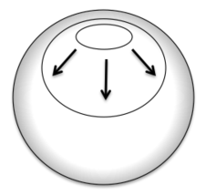
Figure 1: A qualitative picture of the pulsating string motion.

We want to treat the classical string solution representing a pulsating string in $\mathbb{R}\times S^{2}$. The motion of the string is depicted in Figure (1) [10, 11, 12]. We work in conformal gauge and start from the Ansatz for the bosonic string degrees of freedom in $\mathbb{R}\times S^{2}$ ($m=1,2,...$)

$$t=\kappa\,\tau,\qquad\psi=\psi(\tau),\qquad\phi=m\,\sigma\ ,\qquad ds^{2}=-dt^{2}+d\psi^{2}+\sin^{2}\psi\,d\phi^{2}\ .$$ (2.1)

The equation of motion and the conformal gauge constraint (which implies the former for $\dot{\psi}\not=0$) are

$$\ddot{\psi}+m^{2}\,\sin\psi\cos\psi=0\ ,\ \ \ \ \ \ \dot{\psi}^{2}+m^{2}\,\sin^{2}\psi=\kappa^{2}\ .$$ (2.2)

The solution with $\psi(0)=0$ can be written in terms of the Jacobi elliptic function (to have a time-periodic solution we need to assume $\kappa<m$, compatible with the later short string limit ) [13]

$$\sin\psi(\tau)=\frac{\kappa}{m}\,{\rm sn}\Big{(}m\,\tau\,|\,\frac{\kappa^{2}}{m^{2}}\Big{)},\qquad|\sin\psi|\leq\sin\psi_{0}=\frac{\kappa}{m}.$$ (2.3)

The energy and the oscillation number $N=\frac{\sqrt{\lambda}}{2\pi}\oint d\psi\ \dot{\psi}$ (which is the adiabatic invariant associated to $\psi$) are

$$\mathcal{E}_{0} = \frac{E}{\sqrt{\lambda}}=\kappa\ ,$$ (2.4)

$$\mathcal{N} = \frac{N}{\sqrt{\lambda}}=\int^{2\pi}_{0}\frac{d\psi}{2\pi}\sqrt{\kappa^{2}-m^{2}\,\sin^{2}\psi}=\frac{2m}{\pi}\Big{[}\Big{(}\frac{\kappa^{2}}{m^{2}}-1\Big{)}\,\mathbb{K}\Big{(}\frac{\kappa^{2}}{m^{2}}\Big{)}+\mathbb{E}\Big{(}\frac{\kappa^{2}}{m^{2}}\Big{)}\Big{]}\ ,$$ (2.5)

where $\frac{{\sqrt{\lambda}}}{2\pi}$ is string tension, and ${\mathbb{K}}$ and ${\mathbb{E}}$ are the usual elliptic functions [13, 7]. The expansion of $\mathcal{N}$ for small $\kappa$ gives

$$\mathcal{N}=\frac{\kappa^{2}}{2m}+\frac{\kappa^{4}}{16m^{3}}+\frac{3\kappa^{6}}{128m^{5}}+\dots\ .$$ (2.6)

Thus the short string (${\mathcal{N}}\to 0$) expansion of the classical energy reads

$$\mathcal{E}_{0}(\mathcal{N})=\sqrt{2\,m\,\mathcal{N}}\,\Big{(}1-\frac{\mathcal{N}}{8m}-\frac{5\mathcal{N}^{2}}{128m^{2}}+\dots\Big{)}.$$ (2.7)

2.1 Quadratic fluctuations around the pulsating background

In the semiclassical approach, one computes the one loop correction to the energy starting from the quadratic fluctuations around the classical solution. The bosonic fluctuations in conformal gauge describe two mixed modes. They can be decoupled by exploiting the Virasoro constraints. An alternative equivalent approach is based on the static gauge (see for instance [7]).

The conformal gauge fluctuations in $AdS_{5}$ describe a free massless ghost field and four free massive fields with mass $\kappa$. (here $k=1,2,3,4$;   $\partial_{a}\partial^{a}=-\partial_{\tau}^{2}+\partial_{\sigma}^{2}$) The Lagrangian for the five $S^{5}$ fluctuations ($\xi,\eta,z_{1},z_{2},z_{3}$) is

$$L_{S}^{(2)}=\frac{1}{2}(\dot{\xi}^{2}-\xi^{\prime 2}-M_{\xi}^{2}\,\xi^{2})+\frac{1}{2}(\dot{\eta}^{2}-\eta^{\prime 2}-M_{\eta}^{2}\,\eta^{2})+\ m\,\cos\psi\,(\xi\,\eta^{\prime}-\xi^{\prime}\,\eta)$$ (2.8)

$$\ \ \ \ \ \ \ \ \ \ \ \ \ \ +\ \frac{1}{2}(\dot{z}_{i}^{2}-z^{\prime}_{i}{}^{2}-M^{2}z_{i}^{2})\ ,$$ (2.9)

with the following background-dependent masses

$$M^{2}=\kappa^{2}-2m^{2}\,\sin^{2}\psi,\qquad M_{\xi}^{2}=\kappa^{2}+m^{2}\cos(2\psi)\ ,\qquad M_{\eta}^{2}=m^{2}\,\cos(2\psi)\ .$$ (2.10)

The coupled system $(\xi,\eta$) can be shown to be equivalent to a decoupled system of one massless mode and of the massive mode with the Lagrangian

$$L=\frac{1}{2}(\dot{g}^{2}-g^{\prime 2}-\tilde{M}^{2}\,g^{2})\ ,\ \ \ \ \ \ \ \ \ \ \ \ \tilde{M}^{2}=\kappa^{2}\big{(}1-\frac{2}{\sin^{2}\psi}\big{)}\ .$$ (2.11)

Yet another equivalent fluctuation action follows also from the Pohlmeyer reduction approach [21].

The general fermionic fluctuation Lagrangian can be found, e.g., in [14, 7]. Fixing $\kappa$ symmetry as usual with $\theta^{1}=\theta^{2}$, and after some standard manipulation, we can write the (squared) fermionic fluctuation operators for both chiralities as

$$\tilde{D}_{F}^{2}{}_{\pm}=\partial_{\tau}^{2}-\partial_{\sigma}^{2}+M^{2}_{\pm}\ ,\ \ \ \ \ \ \ \ \ \ \ \ M^{2}_{\pm}=\dot{\psi}^{2}\pm i\,\ddot{\psi}.$$ (2.12)

Ultraviolet finiteness is easily checked by computing the supertrace of the squared mass matrix. The signed sum of squared masses turns out to be proportional to $\sqrt{-g}\,R^{(2)}$ , i.e., the Euler density of the induced metric as expected on general grounds [15]. After integration over the 2-space, one finds a vanishing result for the cylinder topology which is appropriate for the string configuration under study.

2.2 Fluctuation operators in Lamé form

We now show that all the obtained one-dimensional spectral problems can be put in standard 1-gap Lamé form (see for instance the detailed discussion in [7]). This is important and means that all their relevant properties can be worked out exactly. Since the fluctuation potentials are independent of the spatial coordinate $\sigma$ for the pulsating string solutions, we Fourier decompose all fields according to $X(\tau,\sigma)=X(\tau)\ e^{in\sigma}$, so that $-\partial_{\tau}^{2}+\partial_{\sigma}^{2}+M^{2}(\tau)\to-\partial_{\tau}^{2}+M^{2}(\tau)-n^{2}$. Depending on the form of the mass term (i.e. potential) $M^{2}(\tau)$, we find three types of Lamé operators, which we discuss below.

2.2.1 Type I operator

The operator associated to the three $S^{5}$ modes $z_{i}$ in (2.9) which have mass $M^{2}=\kappa^{2}-2m^{2}\sin^{2}\psi$ is

$${\cal O}_{I}=-\partial_{\tau}^{2}+2m^{2}\sin^{2}\psi-\kappa^{2}-n^{2}\ .$$ (2.13)

For the pulsating string, Eq. (2.3), it can be written as

$${\cal O}_{I}=m^{2}\,\Big{[}-\partial^{2}_{x}+\ 2k^{2}\,{\rm sn}^{2}(x\,|\,k^{2})-\Lambda\Big{]},$$ (2.14)

$$x=m\,\tau,\qquad{k^{2}=\frac{\kappa^{2}}{m^{2}}},\qquad\Lambda=\frac{\kappa^{2}+n^{2}}{m^{2}}\ ,$$

which is of the single-gap Lamé form.

2.2.2 Type II operator

Next, consider the $S^{5}$ mode in (2.11) with mass $\tilde{M}^{2}=\kappa^{2}\big{(}1-\frac{2}{\sin^{2}\psi}\big{)}$, i.e. with the associated operator

$${\cal O}_{II}=-\partial_{\tau}^{2}+\frac{2\kappa^{2}}{\sin^{2}\psi}-\kappa^{2}-n^{2}=m^{2}\,\Big{[}-\partial^{2}_{x}+\ 2\,{\rm ns}^{2}(x\,|\,k^{2})-\Lambda\Big{]}\ ,$$ (2.15)

where we have used the definitions (2.14). Taking into account the identity, ${\rm ns}(z\,|\,k^{2})=k\,{\rm sn}(z+i\,\mathbb{K}^{\prime}\,|\,k^{2})$, we have (we use the standard notation ${\mathbb{K}}^{\prime}(k^{2})\equiv{\mathbb{K}}(1-k^{2})$)

$${\cal O}_{II} = m^{2}\,\Big{[}-\partial^{2}_{x}+\ 2\,k^{2}\,{\rm sn}^{2}(x\,|\,k^{2})-\Lambda\Big{]},$$ (2.16)

$$x \equiv m\,\tau+i\,\mathbb{K}^{\prime}\quad,\quad k=\frac{\kappa}{m}\quad,\quad\Lambda=\frac{\kappa^{2}+n^{2}}{m^{2}}\quad,$$

which is again of the single-gap Lamé form.

2.2.3 Type III operator

The fermion fluctuation operator in (2.12) with the mass $M^{2}_{\pm}=\dot{\psi}^{2}\pm i\,\ddot{\psi}$ leads to

$${\cal O}_{III}^{\pm}=-\partial_{\tau}^{2}-\dot{\psi}^{2}\mp i\,\ddot{\psi}-n^{2}.$$ (2.17)

After some manipulation of the elliptic functions, we can show that it can be written

$${\cal O}_{III}^{\pm}=\bar{m}_{\pm}^{2}\,\Big{[}-\partial^{2}_{x}+2\,\bar{k}_{\pm}^{2}\,{\rm sn}^{2}(\bar{x}\,|\,\bar{k}_{\pm}^{2})-\Lambda\Big{]}\ ,$$ (2.18)

$$\bar{x}\equiv\bar{m}_{\pm}\,\tau+\frac{1}{2}{{\mathbb{K}}(\bar{k}^{2}_{\pm})}\ ,\qquad\bar{m}_{\pm}=\frac{m}{2}\Big{(}\sqrt{1-\frac{\kappa^{2}}{m^{2}}}\pm i\frac{\kappa}{m}\Big{)}\ ,$$ (2.19)

$$\bar{k}_{\pm}^{2}=\pm 4\frac{\frac{i\,\kappa}{m}\sqrt{1-\frac{\kappa^{2}}{m^{2}}}}{\Big{(}{\sqrt{1-\frac{\kappa^{2}}{m^{2}}}}\pm{\frac{i\kappa}{m}}\Big{)}^{2}}\ ,\qquad\Lambda=\frac{n^{2}}{\bar{m}_{\pm}^{2}+\bar{k}_{\pm}^{2}}\ .$$ (2.20)

Thus we again find a fluctuation operator of the single-gap Lamé form.

3 Semiclassical quantization of time-periodic solutions of integrable systems

Let us consider a classical Hamiltonian system on a space $X$ ($\dim X=2n$) with a Hamiltonian $H:T^{*}X\to\mathbb{R}.$ Its quantum version will be a self-adjoint operator $\widehat{H}$ on such that in the classical limit $\hbar\to 0$ it reduces to $H$. Classical integrability requires the existence of $n$ functions $F_{1},\dots,F_{n}\in C(T^{*}X)$ such that: (i) $dF_{1}\wedge\cdots\wedge dF_{n}\neq 0,\ {\rm almost\ everywhere},$ (ii) $\{F_{i},F_{j}\}=0,$ and (iii) $H=H(F_{1},\dots,F_{n})$. This implies that the level sets define $n$-tori (Liouville tori) foliating $T^{*}X$ and invariant under the Hamiltonian flow. This allows one to define the action variables $I_{i}$ parametrizing the foil base and the angle variables $\varphi_{i}$, the coordinates of the torus. The weaker condition of semiclassical integrability requires the existence of quantum extensions $\widehat{F}_{i}$ of $F_{i}$ ($\widehat{F}_{i}\stackrel{{\scriptstyle\hbar\to 0}}{{\longrightarrow}}F_{i}$) such that in addition to the condition (i) above they satisfy (ii’) $[\widehat{F}_{i},\widehat{F}_{j}]=\mathcal{O}(\hbar^{3})$ and (iii’) $\widehat{H}=H(\widehat{F}_{1},\dots,\widehat{F}_{n})+\mathcal{O}(\hbar^{2})$. Note that $\widehat{H}$ is well defined without ordering problems because of the condition (ii’).

The joint semiclassical diagonalization problem

$$\widehat{F}_{i}\,\psi=f_{i}\,\psi+\mathcal{O}(\hbar^{2})\ ,$$ (3.1)

can be solved by a WKB-like approximation which require the following Bohr-Sommerfeld-Maslov (BSM) quantization condition [16]

$$\frac{1}{2\pi\hbar}\int_{\gamma_{i}}{p}\cdot dq=N_{i}+\frac{\mu_{i}}{4}+\mathcal{O}(\hbar),\qquad i=1,\dots,n\ ,$$ (3.2)

where the integers $N_{i}$ thus define the action variables, $\{\gamma_{i}\}$ is a basis of cycles of a Liouville torus, and the Maslov indices $\mu_{i}$ take into account the critical points of the cycles.

If the classical invariant torus has only $p<n$ non trivial cycles, then the BSM quantization condition must be modified in order to take into account the fluctuations transverse to the codimension $p$ invariant torus. It becomes

$$\frac{1}{2\pi\hbar}\int_{\gamma_{k}}{p}\cdot dq=N_{k}+\frac{\mu_{k}}{4}+\sum_{\alpha=p+1}^{n}\big{(}n_{\alpha}+\frac{1}{2}\big{)}\,\frac{\nu_{\alpha}^{(k)}}{2\pi}+\mathcal{O}(\hbar),\quad\begin{array}[]{l}\ \ \ \ \ k=1,\dots,p,\\ \ \ \ \ \ n_{\alpha}\ll N_{k}\end{array}$$ (3.5)

The stability angles $\nu_{\alpha}^{(k)}$ can be found by studying the stability of small fluctuations around the invariant torus (the condition $n_{\alpha}\ll N_{k}$ is necessary in order to be able to use the linearised analysis).

In the case of semiclassical quantization of finite $g$-gap solutions of string theory, one starts with a classical energy as a function of the action variables and then simply shifts them according to the BSM quantization conditions [9]

$$E=E_{cl}\Big{(}N_{1}\hbar+\frac{\hbar}{2}+\hbar\sum_{\alpha=g+2}^{\infty}\big{(}n_{\alpha}+\frac{1}{2}\big{)}\frac{\nu_{\alpha}^{(1)}}{2\pi},\dots,$$

$$\qquad\qquad N_{g+1}\hbar+\frac{\hbar}{2}+\hbar\sum_{\alpha=g+2}^{\infty}\big{(}n_{\alpha}+\frac{1}{2}\big{)}\frac{\nu_{\alpha}^{(g+1)}}{2\pi}\Big{)}+\mathcal{O}(\hbar^{2})\ .$$ (3.6)

In particular, for the ground state ($n_{\alpha}=0$) of a 1-gap superstring time-dependent solution of period ${\cal T}$, we can write (here $\hbar=\frac{1}{\sqrt{\lambda}}$, $\mathcal{N}=\frac{N}{\sqrt{\lambda}},\ \mathcal{E}=\frac{E}{\sqrt{\lambda}}$)

$$\mathcal{E}=\mathcal{E}_{cl}(\mathcal{N})+\frac{1}{2\sqrt{\lambda}}\frac{1}{{\cal T}}\sum_{\nu_{s}>0}\nu_{s}+\mathcal{O}(\frac{1}{(\sqrt{\lambda})^{2}})\ .$$ (3.7)

Here ${\cal T}$ is the period of the solution which is the inverse of $\frac{dE}{dN}$.

In general, in an integrable system, the stability angles may be computed starting from the problem of evolution of a small perturbation which is controlled by the non-linear superposition principle associated with Bäcklund transformations. The same construction can be interpreted as the addition of an infinitesimal cut to a finite cut solution of the corresponding integral equations implied by the Bethe equations. Also, a third point of view is that of considering a genus $g+1$ algebraic curve infinitesimally near its genus $g$ degeneration point. In the case of the pulsating string, this sophisticated discussion will simply boil down to the nice spectral properties of the Lamé equation.

4 One-loop correction to energy

In general, given the 1-d spectral problem with a periodic potential

$$\big{[}-\partial_{x}^{2}+V(x)\big{]}\,f(x)=\Lambda\,f(x)\ ,\ \ \ \ \ \ \ \ \ \ \ V(x+{\cal T})=V(x)\ ,$$ (4.1)

its two independent solutions $f_{\pm}(x)=e^{\pm i\,p(\Lambda)\,x}\,\chi_{\pm}(x),\ \ \chi_{\pm}(x+{\cal T})=\chi_{\pm}(x)$ satisfy

$$f_{\pm}(x+{\cal T})=e^{\pm i\nu}\ f_{\pm}(x)\ ,\ \ \ \ \ \ \nu=p{\cal T}\ ,$$ (4.2)

where $\nu$ is the “stability angle” and $p$ is the “quasi-momentum” (in general, $p$ is a function of $\Lambda,{\cal T}$ and a functional of $V$).

For the pulsating string in $\mathbb{R}\times S^{2}$ the period is ${\cal T}=\frac{4\mathbb{K}}{m}$. The short string limit is the small $\kappa$ limit, in which the semiclassical oscillation parameter $\mathcal{N}$ is small. Below we shall consider the positive of the two possible stability angles differing by sign (see [17]). Since in the present case the $AdS$ time $t$ and 2d time $\tau$ are related as in (2.1), i.e. $t=\kappa\tau$, there will be similar proportionality of the periods, and the space-time energy and the 2d energy will be related by

$$E_{\rm spacetime}=\frac{1}{\kappa}E_{2d}\ .$$ (4.3)

4.1 Stability angles

The $4$ massless $AdS_{5}$ fluctuations have simply the stability angle

$$\nu_{{}_{AdS_{5}}}=4\mathbb{K}\,\sqrt{k^{2}+\frac{n^{2}}{m^{2}}}\ ,\ \ \ \ \ \ \ \ k\equiv\frac{\kappa}{m}\ .$$ (4.4)

As we have shown, the $S^{5}$ bosonic fluctuations (both Type I (2.13) and Type II (2.15)) are associated with the standard Lamé equation, and therefore the stability angle is

$$\nu_{{}_{S^{5}}}=\pm 4\,\mathbb{K}\,\left(i\,\mathbb{Z}(\alpha\,|\,k^{2})+\frac{\pi}{2\mathbb{K}}\right)\equiv\pm 4\,\mathbb{K}\,i\,\mathbb{Z}(\alpha\,|\,k^{2})\ ,$$ (4.5)

$${\rm sn}(\alpha\,|\,k^{2})=\sqrt{\frac{1+k^{2}-\Lambda}{k^{2}}}=\frac{1}{k}\sqrt{1-\frac{n^{2}}{m^{2}}}\ .$$ (4.6)

We shall fix the sign in (4.5) by the condition $\nu>0$. Finally, in the case of the fermionic fluctuation operator the expression for the stability angle is

$$\nu_{{}_{F}}=\pm 4\,i\,\mathbb{K}\,\Big{[}\frac{1}{2}\,Z(\alpha({\beta})\,|\,k^{2})+i\,\sqrt{\beta}\,\sqrt{1+\frac{16\,\beta\,k^{2}}{(1-4\beta)^{2}}}\ \Big{]},$$ (4.7)

where

$$\alpha(\beta)={\rm cn}^{-1}\Big{(}-\frac{1+4\beta}{1-4\beta}\,|\,k^{2}\Big{)}\ ,\ \ \ \ \ \ \ \ \ \beta=\frac{n^{2}}{m^{2}}\ .$$ (4.8)

Let us now combine the above stability angles expanded in powers of $\kappa={km}$ with proper multiplicities and signs as they should appear in the 1-loop correction to the energy in (3.7)

$${\nu_{n}=4\times(\nu_{{}_{AdS_{5}}}+\nu_{{}_{S^{5}}})-8\times\nu_{{}_{F}}}$$

$$\ \ \ =\frac{4\pi\kappa^{2}m}{n\,(m^{2}-4n^{2})}-\frac{\pi\kappa^{4}(2m^{8}-28m^{6}n^{2}+133m^{4}n^{4}-128m^{2}n^{6}+48n^{8})}{2mn^{3}(m^{2}-4n^{2})^{3}(m^{2}-n^{2})}$$

$$\ \ \ +\ \frac{\pi\kappa^{6}}{16m^{3}(m^{2}-n^{2})^{2}(m^{2}n-4n^{3})^{5}}\Big{(}8m^{16}-180m^{14}n^{2}+1705m^{12}n^{4}-8772m^{10}n^{6}+25883m^{8}n^{8}$$

$$\ \ \ \ \ \ \ \ \ \ \ \ \-\ 35456m^{6}n^{10}+25824m^{4}n^{12}-13824m^{2}n^{14}+3840n^{16}\Big{)}+...\ .$$ (4.9)

As a check, we observe that the sum over $n$ of this combination is convergent at large $n$. Setting $m=1$ and summing up all the contributions we get from (3.7) the following expression for the 1-loop correction to the string energy (taking into account the relation (4.3) valid in the static gauge $t=\kappa\tau$)

$$\mathcal{E}_{1}=\frac{1}{2{\cal T}\kappa}\sum_{n=-\infty}^{\infty}{\nu_{n}} = 2+\kappa(1-4\log 2)+\frac{1}{8}\kappa^{3}\Big{(}{3\zeta_{3}}+{1}+4\log 2\Big{)}$$ (4.10)

$$+\frac{1}{4}\kappa^{5}\Big{(}-\frac{63\zeta_{3}}{16}-\frac{15\zeta_{5}}{16}+\frac{7}{32}+{\log 2}\Big{)}+O(\kappa^{7})\ .$$

In general, we can organize the short string expansion of the energy as

$$E=E\Big{(}\frac{N}{\sqrt{\lambda}},\sqrt{\lambda}\Big{)}=\sqrt{\lambda}\,\mathcal{E}_{0}(\mathcal{N})+\mathcal{E}_{1}(\mathcal{N})+\frac{1}{\sqrt{\lambda}}\,\mathcal{E}_{2}(\mathcal{N})+...\ ,$$ (4.11)

$$\mathcal{E}_{k}=\sqrt{2\mathcal{N}}\ \Big{(}a_{0k}+a_{1k}\,\mathcal{N}+a_{2k}\,\mathcal{N}^{2}+...\Big{)}+c_{0k}+c_{1k}\,\mathcal{N}+....\ .$$ (4.12)

where $c_{nk}$ are coefficients of “non-analytic” terms [18]. Using (2.6),(2.7) and (4.10) we find that for the pulsating string in $\mathbb{R}\times S^{2}$

$$\mathcal{E}_{0} = \sqrt{2\mathcal{N}}\Big{(}1-\frac{1}{8}\mathcal{N}-\frac{5}{128}\mathcal{N}^{2}+...\Big{)},$$ (4.13)

$$E_{1}\equiv\mathcal{E}_{1} = 2+\sqrt{2\mathcal{N}}\Big{[}1-4\log 2+\Big{(}\frac{3}{2}\log 2+\frac{3}{4}\zeta_{3}+\frac{1}{8}\Big{)}\mathcal{N}$$ (4.14)

$$+\ \Big{(}\frac{25}{32}\log 2-\frac{135}{32}\zeta_{3}-\frac{15}{16}\zeta_{5}+\frac{11}{128}\Big{)}\mathcal{N}^{2}+...\Big{]}.$$

Therefore, the energy can be re-written in terms of $N$ and the string tension as follows

$$E=\sqrt{2N\sqrt{\lambda}}\ \Big{(}a_{00}+\frac{a_{10}N+a_{01}}{\sqrt{\lambda}}+...\Big{)}+c_{01}+...\ ,$$ (4.15)

$$a_{00}=1,\qquad a_{10}=-\frac{1}{8},\qquad a_{01}=1-4\log 2,\qquad c_{01}=2\ ,\ \ \ ...$$ (4.16)

5 Generalizations and concluding remarks

In this paper we extended the investigation [7] of the exact structure of one-loop correction to energy of an important class of classical string solutions in $AdS_{5}\times S^{5}$ expressed in terms of elliptic functions. The elliptic solution considered in [7] was the folded spinning string in $AdS_{5}$ for which it was shown that the quadratic fluctuation operators can be put into the standard single-gap Láme form. This is an important feature allowing to compute the one-loop correction to the string energy exactly for any value of semiclassical spin parameter ${\mathcal{S}}$. Here we have extended the calculation to the pulsating string in $\mathbb{R}\times S^{2}$. Additional details as well as the extensions to the pulsating string in $AdS_{3}$ and the folded spinning string in $\mathbb{R}\times S^{2}$ can be found in [19].

In all cases where there is only one charge/adiabatic invariant besides the energy, namely, an oscillator number or spin (in $S^{5}$ or $AdS_{5}$), the fluctuation operators can be decoupled and put into a single-gap Lamé type form.

We focused on the expansion of the one-loop energies in the limit of small values of the semiclassical parameters corresponding to small size of the string. In this limit the string probes only small region of $AdS_{5}\times S^{5}$ so its energy should start with the standard flat-space form plus corrections due to curvature. This limit may provide further insight into the structure of strong-coupling corrections to dimensions of “short” dual gauge theory operators for which the “wrapping” contributions are important [20, 18].

The semiclassical approximation is based on assumption that ${\sqrt{\lambda}}\gg 1$ with semiclassical parameters characterizing the various solutions (see [19], for the precise definitions) like ${\mathcal{S}}=\frac{S}{{\sqrt{\lambda}}},\ {\cal J}=\frac{J}{{\sqrt{\lambda}}}$ or ${\cal N}=\frac{N}{{\sqrt{\lambda}}}$ fixed, so that $S,J$ or $N$ are formally large. An intriguing conjecture is that, taking the “short-string” limit in which ${\mathcal{S}},{\cal J},{\cal N}\to 0$, one may assume that the limit “commutes” with the large ${\sqrt{\lambda}}$ limit. If so, the semiclassical analysis may shed light on the form of the quantum string energies with fixed values of the spins and oscillation numbers $(S,J,N)$. While this is only a conjecture, the study of the “short-string” limit provides some qualitative information on the structure of the large tension expansion of quantum string energies or strong-coupling expansion of dimensions of dual gauge-theory operators.

We summarize below the results for the “short-string” (small spin or oscillation number) expansion of the classical $E_{0}$ and one-loop $E_{1}$ energies of the four basic elliptic $AdS_{5}\times S^{5}$ solutions analysed in [7] and here: folded spinning strings in $\mathbb{R}\times S^{2}$ and $AdS_{3}$, and pulsating circular strings in $\mathbb{R}\times S^{2}$ and $AdS_{3}$. We recall our notation: $E=E_{0}+E_{1}+...$, $E_{0}={\sqrt{\lambda}}\mathcal{E}_{0}$, $E_{1}=\mathcal{E}_{1}$. Also, the non-zero spin of the folded string in $S^{2}$ is $J_{2}\equiv J$.

Folded spinning string in $\mathbb{R}\times S^{2}$

$$\mathcal{E}_{0} = \sqrt{2\,\mathcal{J}}\,\Big{(}1+\frac{1}{8}\,\mathcal{J}+\frac{3}{128}\mathcal{J}^{2}+\dots\Big{)},$$

$$E_{1} = 2+\sqrt{2\,\mathcal{J}}\,\Big{[}2-4\,\log 2+\Big{(}-\frac{1}{2}-\frac{3}{2}\log 2+\frac{3}{4}\zeta_{3}\Big{)}\,\mathcal{J}$$

$$\ \ \ \ \ +\Big{(}\frac{1}{64}-\frac{15}{32}\log 2+\frac{51}{32}\zeta_{3}-\frac{15}{16}\zeta_{5}\Big{)}\,\mathcal{J}^{2}+\dots\Big{]},$$

$$E = \sqrt{2J\sqrt{\lambda}}\Big{(}1+\frac{\frac{1}{8}J+2-4\log 2}{\sqrt{\lambda}}+\dots\Big{)}+2+\dots$$ (5.1)

Folded spinning string in $AdS_{3}$

$$\mathcal{E}_{0} = \sqrt{2\,\mathcal{S}}\,\Big{(}1+\frac{3}{8}\,\mathcal{S}-\frac{21}{128}\mathcal{S}^{2}+\dots\Big{)},$$

$$E_{1} = 1+\sqrt{2\,\mathcal{S}}\,\Big{[}\frac{3}{2}-4\,\log 2+\Big{(}-\frac{23}{16}+\frac{3}{2}\log 2+\frac{3}{4}\zeta_{3}\Big{)}\,\mathcal{S}$$

$$\ \ \ \ \ \ +\Big{(}\frac{689}{256}-\frac{63}{32}\log 2-\frac{15}{32}\zeta_{3}-\frac{15}{16}\zeta_{5}\Big{)}\,\mathcal{S}^{2}+\dots\Big{]},$$

$$E = \sqrt{2S\sqrt{\lambda}}\Big{(}1+\frac{\frac{3}{8}S+\frac{3}{2}-4\log 2}{\sqrt{\lambda}}+\dots\Big{)}+1+\dots$$ (5.2)

Pulsating string in $\mathbb{R}\times S^{2}$

$$\mathcal{E}_{0} = \sqrt{2\,\mathcal{N}}\,\Big{(}1-\frac{1}{8}\,\mathcal{N}-\frac{5}{128}\,\mathcal{N}^{2}+\dots\Big{)},$$

$$E_{1} = 2+\sqrt{2\,\mathcal{N}}\,\Big{[}1-4\,\log 2+\Big{(}\frac{1}{8}+\frac{3}{2}\log 2+\frac{3}{4}\zeta_{3}\Big{)}\,\mathcal{N}$$

$$\ \ \ \ \ +\Big{(}\frac{11}{128}+\frac{25}{32}\log 2-\frac{135}{32}\zeta_{3}-\frac{15}{16}\zeta_{5}\Big{)}\mathcal{N}^{2}+\dots\Big{]},$$

$$E = \sqrt{2N\sqrt{\lambda}}\Big{(}1+\frac{-\frac{1}{8}N+1-4\log 2}{\sqrt{\lambda}}+\dots\Big{)}+2+\dots$$ (5.3)

Pulsating string in $AdS_{3}$

$$\mathcal{E}_{0} = \sqrt{2\,\mathcal{N}}\,\Big{(}1+\frac{5}{8}\,\mathcal{N}-\frac{77}{128}\,\mathcal{N}^{2}+\dots\Big{)},$$

$$E_{1} = 1+\sqrt{2\,\mathcal{N}}\,\Big{[}\frac{5}{2}-4\log 2+\Big{(}-\frac{37}{8}+\frac{5}{2}\log 2+\frac{3}{4}\zeta_{3}\Big{)}\,\mathcal{N}$$

$$\ \ \ \ \ +\Big{(}\frac{3915}{256}-\frac{231}{32}\log 2-\frac{117}{32}\zeta_{3}-\frac{15}{16}\zeta_{5}\Big{)}\,\mathcal{N}^{2}+\dots\Big{]},$$

$$E = \sqrt{2N\sqrt{\lambda}}\Big{(}1+\frac{\frac{5}{8}N+\frac{5}{2}-4\log 2}{\sqrt{\lambda}}+\dots\Big{)}+1+\dots$$ (5.4)

We observe a remarkable universality of the small charge expansion of the energy of all four elliptic solutions: the leading terms with transcendental coefficients ($\log 2,\ \zeta_{3},\ \zeta_{5},...$) happen to have the same form.

Strings with lowest non-trivial values of the charges should correspond to string states at the first excited level. Since these should be dual to members of the Konishi multiplet, they should have the same anomalous dimension [18]. The relationship between this intriguing universality, the $PSU(2,2|4)$ structure of the Konishi multiplet, and the validity of the above mentioned conjecture remains to be clarified.

References

• [1]
• [2]
• [3] D. Serban, Integrability and the AdS/CFT correspondence, arXiv:1003.4214.
• [4] N. Gromov, Y-system and Quasi-Classical Strings, JHEP 1001, 112 (2010) [arXiv:0910.3608].
• [5] N. Gromov and P. Vieira, Complete 1-loop test of AdS/CFT, JHEP 0804, 046 (2008) [arXiv:0709.3487]. N. Gromov, S. Schafer-Nameki and P. Vieira, Efficient precision quantization in AdS/CFT, JHEP 0812, 013 (2008) [arXiv:0807.4752]. N. Gromov, Integrability in AdS/CFT correspondence: Quasi-classical analysis, J. Phys. A 42, 254004 (2009).
• [6] S. Frolov and A. A. Tseytlin, Multi-spin string solutions in $AdS_{5}\times S^{5}$, Nucl. Phys. B 668, 77 (2003) [arXiv:hep-th/0304255].
• [7] M. Beccaria, G. V. Dunne, V. Forini, M. Pawellek and A. A. Tseytlin, Exact computation of one-loop correction to energy of spinning folded string in $AdS_{5}\times S^{5}$, J. Phys. A 43, 165402 (2010) [arXiv:1001.4018].
• [8] R. F. Dashen, B. Hasslacher and A. Neveu, The Particle Spectrum In Model Field Theories From Semiclassical Functional Integral Techniques, Phys. Rev.  D 11, 3424 (1975).
• [9] B. Vicedo, Semiclassical Quantisation of Finite-Gap Strings, JHEP 0806, 086 (2008) [arXiv:0803.1605]; Finite-g Strings, arXiv:0810.3402.
• [10] S. S. Gubser, I. R. Klebanov and A. M. Polyakov, A semi-classical limit of the gauge/string correspondence, Nucl. Phys.  B 636, 99 (2002) [arXiv:hep-th/0204051].
• [11] J. A. Minahan, Circular semiclassical string solutions on $AdS_{5}\times S^{5}$, Nucl. Phys.  B 648, 203 (2003) [arXiv:hep-th/0209047].
• [12] M. Kruczenski and A. A. Tseytlin, Semiclassical relativistic strings in S5 and long coherent operators in N = 4 SYM theory, JHEP 0409, 038 (2004) [arXiv:hep-th/0406189].
• [13] E.T. Whittaker, G.N. Watson, A course of modern analysis, Cambridge University Press, 4th edition (1927).
• [14] S. Frolov and A. A. Tseytlin, Semiclassical quantization of rotating superstring in $AdS_{5}\times S^{5}$, JHEP 0206, 007 (2002) [arXiv:hep-th/0204226].
• [15] N. Drukker, D. J. Gross and A. A. Tseytlin, Green-Schwarz string in $AdS_{5}\times S^{5}$: Semiclassical partition function, JHEP 0004, 021 (2000) [arXiv:hep-th/0001204].
• [16] A. Voros, The WKB-Maslov method for nonseparable systems, Coll. Inst. CNRS 237, Geom. Sympl. et. Phys. Math., p217 (1974); Semiclassical approximations, Ann. Inst. Henri Poincare 14, 31 (1976).
• [17] B. Hasslacher and A Neveu, Non-linear quantum field theory, Rocky Mountain Journ. Math. 8, 1 (1978); R. Jackiw, Quantum Meaning Of Classical Field Theory, Rev. Mod. Phys.  49, 681 (1977). S. Coleman, Aspects of Symmetry, Cambridge University Press (1988); R. Rajaraman, Solitons And Instantons. An Introduction To Solitons And Instantons In Quantum Field Theory, (North Holland, Amsterdam, 1982).
• [18] R. Roiban and A. A. Tseytlin, Quantum strings in $AdS_{5}\times S^{5}$: strong-coupling corrections to dimension of Konishi operator, JHEP 0911, 013 (2009) [arXiv:0906.4294].
• [19] M. Beccaria, G. V. Dunne, G. Macorini et al., Exact computation of one-loop correction to energy of pulsating strings in $AdS_{5}\times S^{5}$ , [arXiv:1009.2318 [hep-th]].
• [20] A. Tirziu and A. A. Tseytlin, Quantum corrections to energy of short spinning string in $AdS_{5}$, Phys. Rev.  D 78, 066002 (2008) [arXiv:0806.4758].
• [21] Y. Iwashita, One-loop corrections to $AdS_{5}\times S^{5}$ superstring partition function via Pohlmeyer reduction, J. Phys. A 43, 345403 (2010) [arXiv:1005.4386 [hep-th]].