Study of the $K^{+}\pi^{+}\pi^{-}$ Final State in $B^{+}\rightarrow J/\psi K^{+}\pi^{+}\pi^{-}$ and $B^{+}\rightarrow\psi^{\prime}K^{+}\pi^{+}\pi^{-}$

Abstract

Using $535\times 10^{6}$ $B$-meson pairs collected by the Belle detector at the KEKB $e^{+}e^{-}$ collider, we measure branching fractions of $(7.16\pm 0.10{\mathrm{(stat)}}\pm 0.60{\mathrm{(syst)}})\times 10^{-4}$ for $B^{+}\to J/\psi K^{+}\pi^{+}\pi^{-}$ and $(4.31\pm 0.20{\mathrm{(stat)}}\pm 0.50{\mathrm{(syst)}})\times 10^{-4}$ for $B^{+}\to\psi^{\prime}K^{+}\pi^{+}\pi^{-}$. We perform amplitude analyses to determine the resonant structure of the $K^{+}\pi^{+}\pi^{-}$ final state in $B^{+}\to J/\psi K^{+}\pi^{+}\pi^{-}$ and $B^{+}\to\psi^{\prime}K^{+}\pi^{+}\pi^{-}$ and find that the $K_{1}(1270)$ is a prominent component of both decay modes. There is significant interference among the different intermediate states, which leads, in particular, to a striking distortion of the $\rho$ line shape due to the $\omega$. Based on the results of the fit to the $B^{+}\to J/\psi K^{+}\pi^{+}\pi^{-}$ data, the relative decay fractions of the $K_{1}(1270)$ to $K\rho$, $K\omega$, and $K^{*}(892)\pi$ are consistent with previous measurements, but the decay fraction to $K_{0}^{*}(1430)$ is significantly smaller. Finally, by floating the mass and width of the $K_{1}(1270)$ in an additional fit of the $B^{+}\to J/\psi K^{+}\pi^{+}\pi^{-}$ data, we measure a mass of $(1248.1\pm 3.3{\mathrm{(stat)}}\pm 1.4{\mathrm{(syst)}})~{}{\mathrm{MeV}}/c^{2}$ and a width of $(119.5\pm 5.2{\mathrm{(stat)}}\pm 6.7{\mathrm{(syst)}})~{}{\mathrm{MeV}}/c^{2}$ for the $K_{1}(1270)$.

I Introduction

The large number of $B$-meson decays observed at $B$ factories allows detailed studies of the intermediate-state resonances involved in these decays. This paper analyzes the structure of the $K^{+}\pi^{+}\pi^{-}$ final state in the decays $B^{+}\rightarrow J/\psi K^{+}\pi^{+}\pi^{-}$ and $B^{+}\rightarrow\psi^{\prime}K^{+}\pi^{+}\pi^{-}$. Kaon excitations that decay to a $K\pi\pi$ final state are difficult to distinguish based on the mass of the $K\pi\pi$ system alone, owing to their overlapping line shapes. In this analysis, data are therefore fitted in the three dimensions $M^{2}(K\pi\pi)$, $M^{2}(K\pi)$, and $M^{2}(\pi\pi)$, which are the squared invariant masses of the $K^{+}\pi^{+}\pi^{-}$, $K^{+}\pi^{-}$ and $\pi^{+}\pi^{-}$ systems, respectively. An unbinned maximum-likelihood fit is performed to extract maximal information from the data. The fitting model accounts for interferences among different intermediate states, as well as the spin-dependent angular distributions of the final state. The large sample size, combined with the clean environment afforded by the presence of a $J/\psi$ or $\psi^{\prime}$ in the final state, makes it possible to distinguish the different kaon excitations that contribute to the $K^{+}\pi^{+}\pi^{-}$ final state. The results provide information not only on intermediate-state interactions but also on the structure of the kaon spectrum. By performing an additional fit in which the mass and width of the $K_{1}(1270)$ are floated, we measure the mass and width of the $K_{1}(1270)$.

Identifying the kaon excitations involved in $B^{+}\rightarrow J/\psi K^{+}\pi^{+}\pi^{-}$ and $B^{+}\rightarrow\psi^{\prime}K^{+}\pi^{+}\pi^{-}$ can lead to a better understanding of the underlying theory. For example, the breaking of $SU(3)$ flavor symmetry mixes the $1^{3}P_{1}$ and $1^{1}P_{1}$ states of the kaon system into the physical states $K_{1}(1270)$ and $K_{1}(1400)$ as

$$K_{1}(1270) = K(1^{3}P_{1})\sin\theta_{K}+K(1^{1}P_{1})\cos\theta_{K},$$ (1)

$$K_{1}(1400) = K(1^{3}P_{1})\cos\theta_{K}-K(1^{1}P_{1})\sin\theta_{K},$$ (2)

where $\theta_{K}$ is the ${}^{3}P_{1}$-${}^{1}P_{1}$ mixing angle. The value of $\theta_{K}$ can be related to the masses of the $K_{1}(1270)$ and $K_{1}(1400)$, to the strong decays of the $K_{1}(1270)$ and $K_{1}(1400)$, and to rates of weak decays to final states involving the $K_{1}(1270)$ and $K_{1}(1400)$ suzuki:1993 ; suzuki:1994 ; blundell:1996 . The measurements presented here can lead to a better determination of $\theta_{K}$.

The data sample used in this study was produced by the KEKB asymmetric-energy $e^{+}e^{-}$ collider kekb and reconstructed by the Belle detector belle_detector . It corresponds to an integrated luminosity of $492~{}{\mathrm{fb}}^{-1}$ accumulated at the $\Upsilon(4S)$ resonance and contains $535\times 10^{6}$ $B\bar{B}$ meson pairs.

II The Belle detector

The Belle detector belle_detector is a large-solid-angle magnetic spectrometer. A silicon vertex detector surrounds the interaction point and reconstructs decay vertices. A $50$-layer central drift chamber (CDC) provides charged-particle tracking over the laboratory polar-angle region $17^{\circ}\leq\theta\leq 150^{\circ}$, which corresponds to $92\%$ of the solid angle in the $\Upsilon(4S)$ rest frame. A system of $1188$ aerogel Cherenkov counters (ACC) and an array of 128 time-of-flight counters provide particle identification. An electromagnetic calorimeter, comprising $8736$ CsI(Tl) crystals, records the energy deposited by photons, leptons, and hadrons. These subdetectors are surrounded by a superconducting solenoid $3.4~{}{\mathrm{m}}$ in diameter and $4.4~{}{\mathrm{m}}$ in length, which produces a $1.5$-${\mathrm{T}}$ magnetic field parallel to the positron beam. An iron flux return installed outside the coil is instrumented with large-area resistive-plate counters to identify muons and $K_{L}$ mesons. Monte Carlo (MC) simulations are used to determine the acceptance of the detector for the processes of interest.

III Event selection

Electron candidates are identified by combining information from the CDC, electromagnetic calorimeter, and ACC. Muon candidates are identified by extrapolating charged-particle tracks from the silicon vertex detector and CDC into the $K_{L}/\mu$ detector. To identify charged hadrons, momentum measurements from the CDC are combined with velocity information from the time-of-flight counters, ACC, and CDC ($dE/dx$) nakano:2002 . The kaon identification efficiency is above $80\%$, while the probability of misidentifying a pion as a kaon is below $10\%$.

Low-momentum charged tracks that curl up in the CDC can be reconstructed multiple times by the track finder. To ensure that no track is included more than once, criteria similar to those of Ref. thesis:hidekazu_kakuno:2003, are used.

In studying a mode that has a $J/\psi$ or $\psi^{\prime}$ in the final state, a key strategy is to reconstruct the $J/\psi$ only in its decays to $e^{+}e^{-}$ or $\mu^{+}\mu^{-}$, and the $\psi^{\prime}$ only in its decays to $e^{+}e^{-}$, $\mu^{+}\mu^{-}$, or $J/\psi\pi^{+}\pi^{-}$. Although this choice abandons all but $12\%$ of $J/\psi$’s and $5\%$ of $\psi^{\prime}$’s, it reduces continuum backgrounds to a negligible level. The decays $J/\psi\rightarrow\mu^{+}\mu^{-}$ and $\psi^{\prime}\rightarrow\mu^{+}\mu^{-}$ are reconstructed by combining oppositely-charged muon candidates. The invariant-mass distribution is then fitted, modeling the $J/\psi$ and $\psi^{\prime}$ as double Gaussians. Muon pairs are discarded unless they have an invariant mass within $\pm 3\sigma$ of the fitted $J/\psi$ or $\psi^{\prime}$ mean, where $\sigma$ is the width of the narrower Gaussian. Similarly, $J/\psi\rightarrow e^{+}e^{-}$ and $\psi^{\prime}\rightarrow e^{+}e^{-}$ decays are reconstructed by combining oppositely-charged electron candidates. To account for energy losses due to final-state radiation or bremsstrahlung in the detector, any photons detected within $50~{}{\mathrm{mrad}}$ of the initial direction of an electron candidate are also included in the $e^{+}e^{-}$ invariant-mass calculation. Electron pairs are discarded unless they have an invariant mass within the range extending from $-4\sigma$ to $+3\sigma$ of the fitted $J/\psi$ or $\psi^{\prime}$ mean. This mass window is asymmetric about the mean so as to include the radiative tails of the $J/\psi$ and $\psi^{\prime}$, which are not completely recovered by the photon addition.

Lepton track pairs that survive the mass requirements are fitted to a common vertex, which is constrained within errors to the measured interaction point. This vertex is then fixed, and another fit is performed, constraining the dilepton invariant mass to the nominal $J/\psi$ or $\psi^{\prime}$ mass. Since the observed widths of the $J/\psi$ and $\psi^{\prime}$ are dominated by measurement error, this procedure improves the mass resolution of the $B$ candidate.

To reconstruct $\psi^{\prime}\rightarrow J/\psi\pi^{+}\pi^{-}$ decays, leptonic $J/\psi$ candidates are combined with a pair of oppositely-charged tracks that satisfy pion-identification criteria. As the $\pi^{+}\pi^{-}$ invariant-mass distribution in $\psi^{\prime}\rightarrow J/\psi\pi^{+}\pi^{-}$ decays is known to peak at high values coffman:1992 , the dipion invariant mass is required to be greater than $0.4~{}{\mathrm{GeV}}/c^{2}$. Unless they have an invariant mass within $\pm 3\sigma$ of the fitted $\psi^{\prime}$ mean, $\psi^{\prime}\rightarrow J/\psi\pi^{+}\pi^{-}$ candidates are discarded.

To reconstruct $B$-meson candidates, each $J/\psi$ or $\psi^{\prime}$ candidate is combined with a kaon candidate and two oppositely-charged pion candidates. Kaon and pion candidates are charged tracks that satisfy identification criteria for kaons and pions, respectively, and have an impact parameter with respect to the fitted dilepton vertex of $|dr|<0.4~{}{\mathrm{cm}}$ and $|dz|<1.5~{}{\mathrm{cm}}$. Any pion candidate that is identified as the product of a $K_{S}^{0}\rightarrow\pi^{+}\pi^{-}$ decay is discarded.

III.1 $B$-Meson reconstruction

Two kinematic variables can be used to identify $B$ mesons. First, the reconstructed mass of a true $B$ meson is likely to fall near the nominal $B$ mass. Second, as $B$ mesons are produced in the reaction

$$e^{+}e^{-}\rightarrow\Upsilon(4S)\rightarrow B^{+}B^{-},$$ (3)

the energy of each $B$ in the $\Upsilon(4S)$ frame is half the total energy of the electron and positron beams in this frame. Since beam-energy drifts can cause the mass of the $\Upsilon(4S)$ to vary, it is customary to recast these kinematic variables in forms that are readily corrected for drifts in the beam energy—namely, the energy difference $\Delta E$ and beam-constrained mass $M_{\mathrm{bc}}$:

$$\Delta E=E^{*}(B)-E_{\mathrm{beam}}^{*},$$ (4)

$$M_{\mathrm{bc}}=\sqrt{E_{\mathrm{beam}}^{*2}-P^{*2}(B)}.$$ (5)

Here, $P^{*}(B)$ is the momentum of the $B$ candidate in the $\Upsilon(4S)$ frame, while $E_{\mathrm{beam}}^{*}$ is half the energy of the $\Upsilon(4S)$ and is measured independently. For a correctly-reconstructed $B$ meson, $\Delta E$ peaks at zero, and $M_{\mathrm{bc}}$ peaks at the nominal $B$ mass.

In the case of a multiparticle final state such as $J/\psi K^{+}\pi^{+}\pi^{-}$ or $\psi^{\prime}K^{+}\pi^{+}\pi^{-}$, multiple $B$ candidates can pose a challenge. If a correctly-reconstructed $B$ candidate includes a low-momentum pion, then an additional $B$ candidate can be formed by replacing that pion with a low-momentum pion from the other $B$. As the exchange does not significantly affect the energy or momentum of the $B$ candidate, both candidates can satisfy $\Delta E$ and $M_{\mathrm{bc}}$ criteria. Multiple candidates can spoil branching-fraction measurements and distort observed mass spectra. To ensure that no $B$ decay is counted more than once, a best-candidate selection is performed. First, $B$ candidates are required to have $|\Delta E|<0.2~{}{\mathrm{GeV}}$ and $M_{\mathrm{bc}}>5.27~{}{\mathrm{GeV}}/c^{2}$. This leaves $25\%$ of $B^{+}\rightarrow J/\psi K^{+}\pi^{+}\pi^{-}$ events and $34\%$ of $B^{+}\rightarrow\psi^{\prime}K^{+}\pi^{+}\pi^{-}$ events with multiple candidates; these events have a mean multiplicity of $2.4$ and $2.7$, respectively. If a given event has multiple $B$ candidates with the same final state, the charged tracks that make up each $B$ candidate are fitted to a common vertex. The candidate whose vertex fit has the smallest $\chi^{2}$ is selected. According to MC studies, this procedure identifies the correct $B$ candidate in approximately $55\%$ of cases where there are multiple candidates.

In the case of $B^{+}\rightarrow J/\psi K^{+}\pi^{+}\pi^{-}$, the decay $B^{+}\rightarrow\psi^{\prime}K^{+}$ is vetoed by rejecting all $B$ candidates that have a $J/\psi\pi^{+}\pi^{-}$ invariant mass between $3.675~{}{\mathrm{GeV}}/c^{2}$ and $3.695~{}{\mathrm{GeV}}/c^{2}$. According to MC studies, $1.1\%$ of $B^{+}\rightarrow\psi^{\prime}K^{+}$ events in which the $\psi^{\prime}$ decays to $J/\psi\pi^{+}\pi^{-}$ and the $J/\psi$ decays to $e^{+}e^{-}$ or $\mu^{+}\mu^{-}$ survive this veto.

III.2 Signal and sideband regions

Data distributions of $\Delta E$ for $B^{+}\rightarrow J/\psi K^{+}\pi^{+}\pi^{-}$ and $B^{+}\rightarrow\psi^{\prime}K^{+}\pi^{+}\pi^{-}$ are shown in Fig. 1. The signal is modeled as a double Gaussian with a single mean, fixing the width and relative height of the wider Gaussian to the results of a MC fit. The background is modeled as a first-order polynomial. Based on these fits, the signal region is defined as

$$-3\sigma_{\Delta E}<\Delta E-\mu_{\Delta E}<+3\sigma_{\Delta E},$$ (6)

where $\mu_{\Delta E}$ is the mean of the signal peak, and $\sigma_{\Delta E}$ is the width of the narrower Gaussian. The sideband region, which is used to estimate the background under the signal, is defined as

$$-0.13~{}{\mathrm{GeV}} <\Delta E-\mu_{\Delta E}< -0.05~{}{\mathrm{GeV}},$$

$$0.05~{}{\mathrm{GeV}} <\Delta E-\mu_{\Delta E}< 0.13~{}{\mathrm{GeV}}.$$ (7)

The sideband normalization factor is given by

$$f_{B}~{}=~{}\frac{\int\limits_{\mathrm{signal}}p_{\mathrm{bkg}}\,d\Delta E}{\int\limits_{\mathrm{sideband}}p_{\mathrm{bkg}}\,d\Delta E},$$ (8)

where $p_{\mathrm{bkg}}$ is the polynomial representing the background. The fraction of signal-region events that are background is estimated as

$$n_{B}~{}=~{}\frac{B}{S}~{}f_{B},$$ (9)

where $S$ and $B$ are the numbers of events in the signal and sideband regions, respectively.

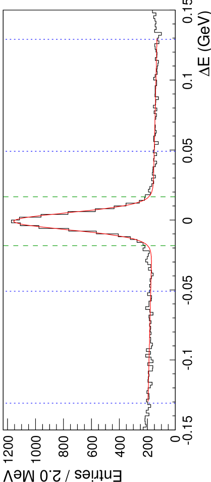
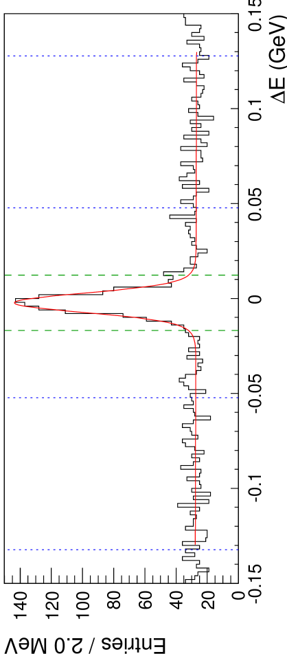
Figure 1: Data $\Delta E$ distributions for $B^{+}\rightarrow J/\psi K^{+}\pi^{+}\pi^{-}$ (top) and $B^{+}\rightarrow\psi^{\prime}K^{+}\pi^{+}\pi^{-}$ (bottom). The curves show the results of the fits described in the text. Dashed and dotted lines indicate the signal and sideband regions, respectively.

IV Coordinate transformations

The data in the sideband region are used to model the background in the signal region. Figure 2, which shows the distribution of $M(K\pi\pi)$ for $B^{+}\rightarrow J/\psi K^{+}\pi^{+}\pi^{-}$ events in the signal and sideband regions, reveals a problem: signal and sideband data have different end points in $M(K\pi\pi)$.

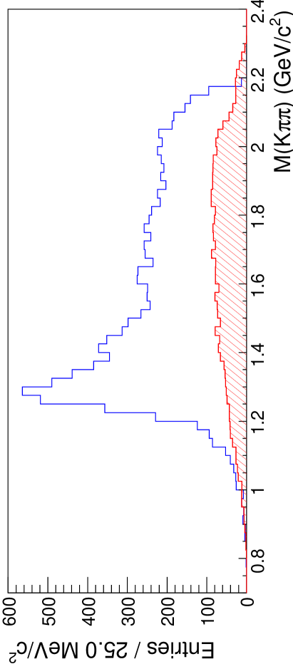
Figure 2: Invariant mass of the $K^{+}\pi^{+}\pi^{-}$ system in $B^{+}\rightarrow J/\psi K^{+}\pi^{+}\pi^{-}$ data. Open and filled histograms show events in the signal and normalized sideband regions, respectively.

Plotting $\Delta E$ versus $M(K\pi\pi)$ reveals the cause of the discrepancy. As Fig. 3 demonstrates, the kinematically allowed range of $M(K\pi\pi)$ depends on $\Delta E$. While the minimum value of $M(K\pi\pi)$ is $M(K\pi\pi)_{\mathrm{min}}=M_{K}+2M_{\pi}$, the maximum value, which is attained when both the $K^{+}\pi^{+}\pi^{-}$ system and the $J/\psi$ are at rest in the $B$-candidate’s rest frame, varies with $\Delta E$ as $M(K\pi\pi)_{\mathrm{max}}=\Delta E+M_{B}-M_{J/\psi}$. Here, $M_{K}$, $M_{\pi}$, $M_{B}$ and $M_{J/\psi}$ stand for the nominal masses of the subscripted particles.

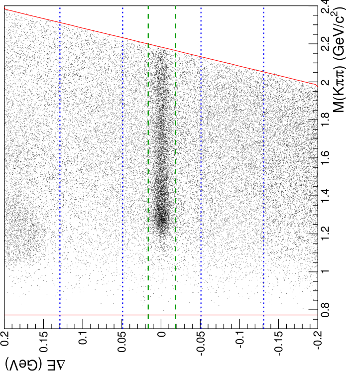
Figure 3: $\Delta E$ versus $M(K\pi\pi)$ for $B^{+}\rightarrow J/\psi K^{+}\pi^{+}\pi^{-}$ data. Dashed lines outline the signal region, and dotted lines outline the sidebands. The solid lines indicate the minimum and maximum values of $M(K\pi\pi)$.

Transforming $M(K\pi\pi)$ as follows removes its dependence on $\Delta E$:

$$M^{\prime}(K\pi\pi) = M(K\pi\pi)_{\mathrm{min}}$$ (10)

$$+ \left[M(K\pi\pi)-M(K\pi\pi)_{\mathrm{min}}\right]$$

$$\times \frac{M(K\pi\pi)_{\mathrm{max}}^{0}-M(K\pi\pi)_{\mathrm{min}}}{M(K\pi\pi)_{\mathrm{max}}-M(K\pi\pi)_{\mathrm{min}}}.$$

Here, $M(K\pi\pi)_{\mathrm{max}}^{0}=M_{B}-M_{J/\psi}$ is the value of $M(K\pi\pi)_{\mathrm{max}}$ at $\Delta E=0$. Figure 4 shows $\Delta E$ versus the transformed coordinate $M^{\prime}(K\pi\pi)$. While the minimum value of $M(K\pi\pi)$ is unaffected by the transformation, the maximum value is changed such that the maximum of $M^{\prime}(K\pi\pi)$ at any $\Delta E$ is equal to the maximum of $M(K\pi\pi)$ at $\Delta E=0$. The range of $M(K\pi\pi)$ is compressed for positive values of $\Delta E$ and stretched for negative values of $\Delta E$.

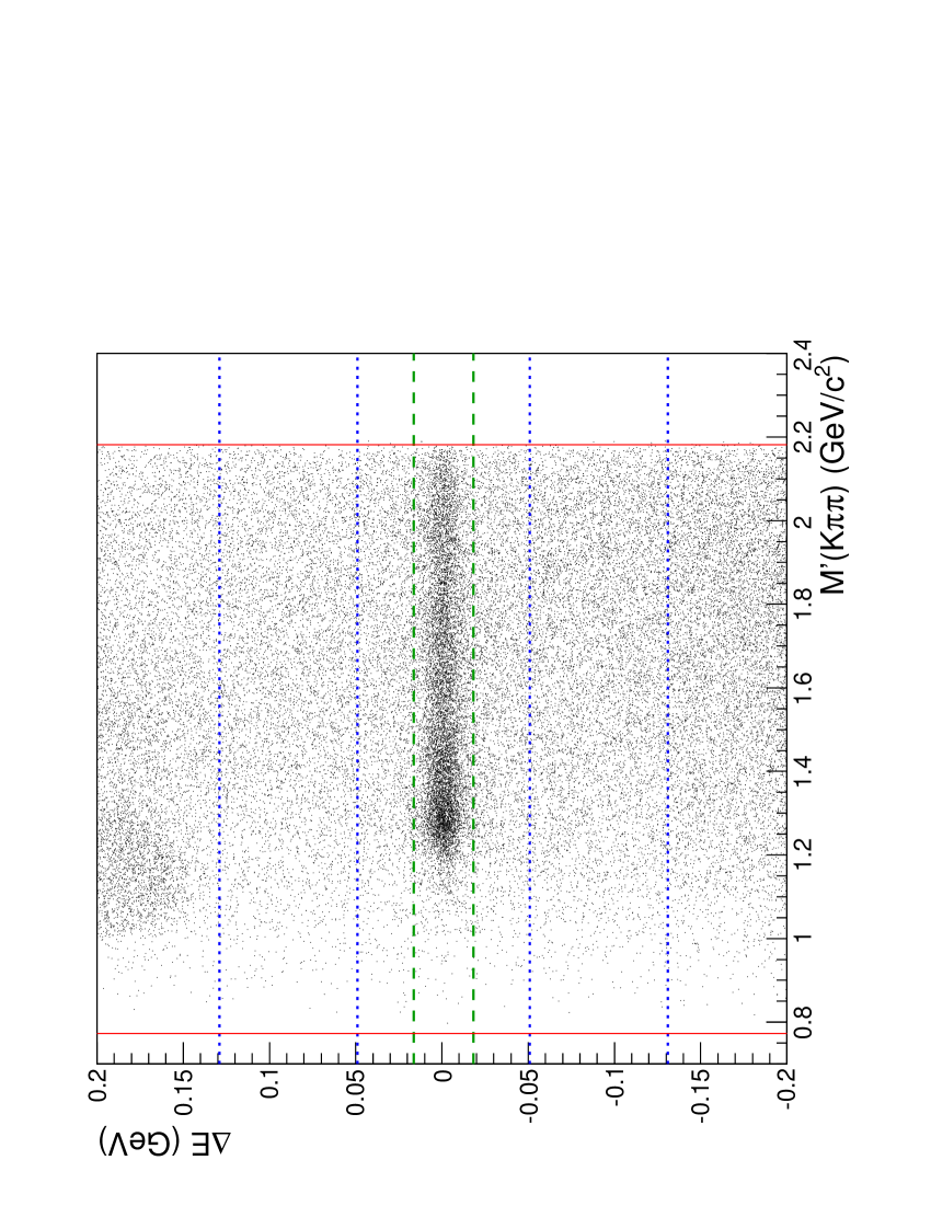
Figure 4: $\Delta E$ versus $M^{\prime}(K\pi\pi)$ for $B^{+}\rightarrow J/\psi K^{+}\pi^{+}\pi^{-}$ data. The lines are defined as in Fig. 3.

Figure 5 shows $M^{\prime}(K\pi\pi)$ for events in the signal and sideband regions. The problem of Fig. 2 has been solved: the end points of the transformed signal and sideband distributions match.

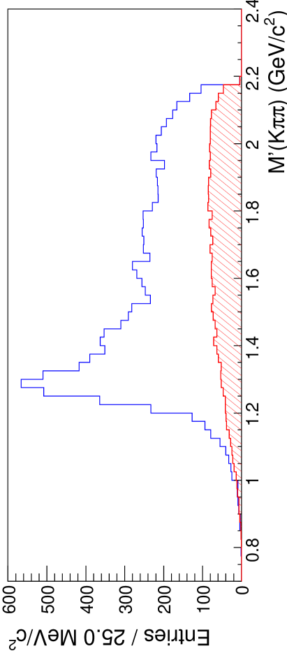
Figure 5: Transformed invariant mass of the $K^{+}\pi^{+}\pi^{-}$ system in $B^{+}\rightarrow J/\psi K^{+}\pi^{+}\pi^{-}$ data. Open and filled histograms show events in the signal and normalized sideband regions, respectively.

An important feature of the transformation is that it does not change $M(K\pi\pi)$ at $\Delta E=0$. Thus, although sideband and signal regions are both transformed, the change is minimal in the signal region.

Just as the range of $M(K\pi\pi)$ depends on $\Delta E$, the ranges of $M(K\pi)$ and $M(\pi\pi)$ also depend on $\Delta E$. To correct for this dependence, transformations similar to Eq. 10 are applied. The variable $M(K\pi)$ is transformed as

$$M^{\prime}(K\pi) = M(K\pi)_{\mathrm{min}}$$ (11)

$$+ \left[M(K\pi)-M(K\pi)_{\mathrm{min}}\right]$$

$$\times \frac{M(K\pi\pi)_{\mathrm{max}}^{0}-M(K\pi\pi)_{\mathrm{min}}}{M(K\pi\pi)_{\mathrm{max}}-M(K\pi\pi)_{\mathrm{min}}},$$

and the variable $M(\pi\pi)$ is transformed as

$$M^{\prime}(\pi\pi) = M(\pi\pi)_{\mathrm{min}}$$ (12)

$$+ \left[M(\pi\pi)-M(\pi\pi)_{\mathrm{min}}\right]$$

$$\times \frac{M(K\pi\pi)_{\mathrm{max}}^{0}-M(K\pi\pi)_{\mathrm{min}}}{M(K\pi\pi)_{\mathrm{max}}-M(K\pi\pi)_{\mathrm{min}}}.$$

Here, $M(K\pi)_{\mathrm{min}}=M_{K}+M_{\pi}$, and $M(\pi\pi)_{\mathrm{min}}=2M_{\pi}$. Figures 6 and 7 show $\Delta E$ versus $M(K\pi)$ and $M^{\prime}(K\pi)$. A similar effect is observed for $M(\pi\pi)$ and $M^{\prime}(\pi\pi)$.

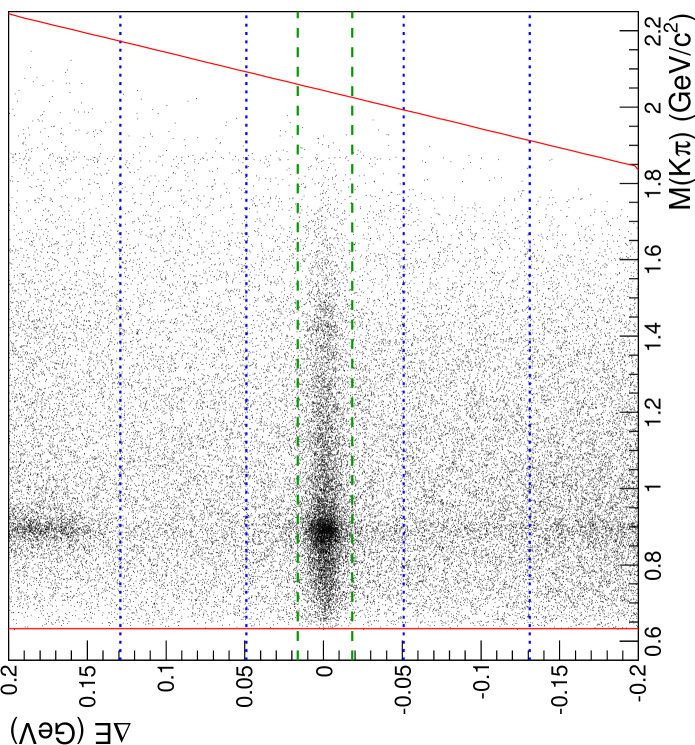
Figure 6: $\Delta E$ versus $M(K\pi)$ for $B^{+}\rightarrow J/\psi K^{+}\pi^{+}\pi^{-}$ data. The lines are defined as in Fig. 3. The concentration of events near $0.9$ GeV$/c^{2}$ represents random particle combinations containing real $K^{*}(892)$s.

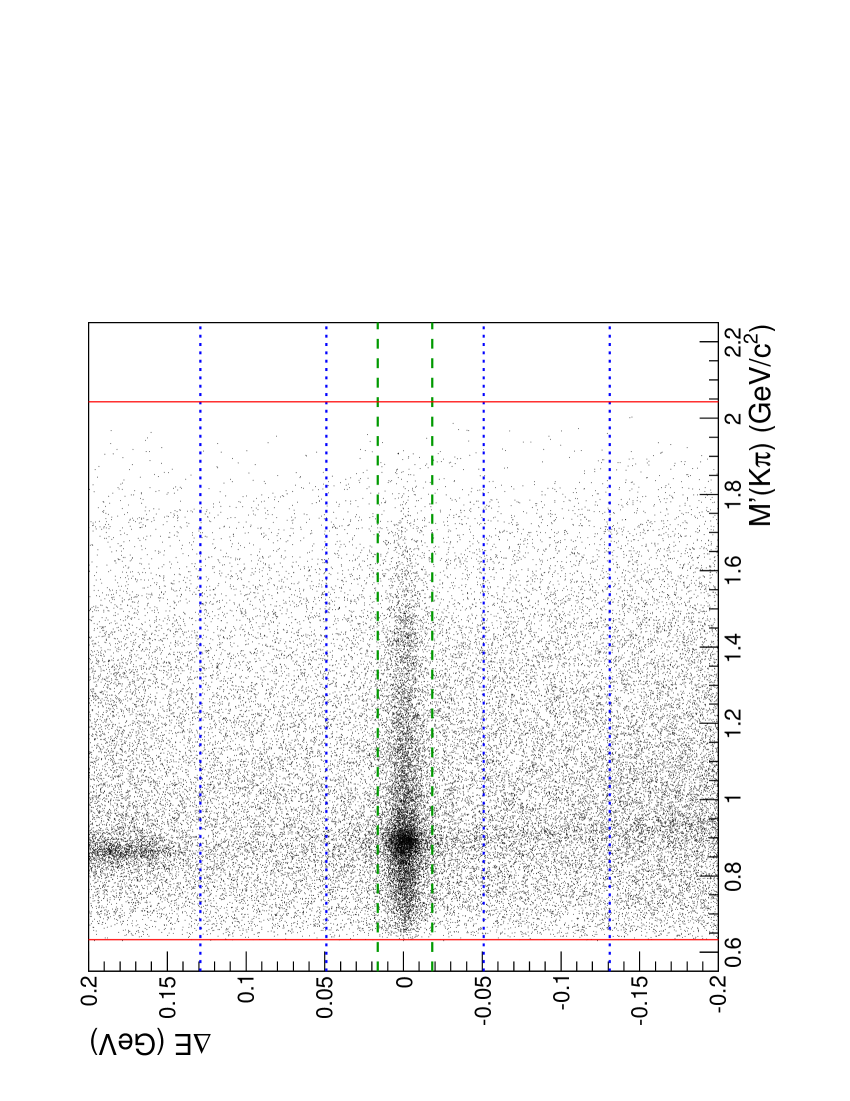
Figure 7: $\Delta E$ versus $M^{\prime}(K\pi)$ for $B^{+}\rightarrow J/\psi K^{+}\pi^{+}\pi^{-}$ data. The lines are defined as in Fig. 3.

As Fig. 7 illustrates, transforming the $M(K\pi)$ coordinate distorts the shapes of the $K^{*}(892)$ and $D^{0}$ backgrounds. This distortion must be taken into account in parametrizing the background for the three-dimensional fits of Sec. VI (i.e., in Eqs. 24 and 25). Modeling the distortion is straightforward. First, the peak is described as a Breit-Wigner or Gaussian in the untransformed coordinate, $M(K\pi)$. Using Eq. 11, $M(K\pi)$ is then written as a function of $M^{\prime}(K\pi)$ and $\Delta E$. The expression is numerically integrated over the relevant range of $\Delta E$ to obtain the shape of the peak as a function of $M^{\prime}(K\pi)$. Figure 8 demonstrates the transformation of the $K^{*}(892)$ background shape.

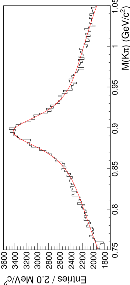
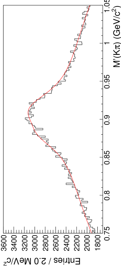
Figure 8: $M(K\pi)$ (top) and $M^{\prime}(K\pi)$ (bottom) distributions of the $K^{*}(892)$ peak in generic-MC sidebands. The curve in the top plot is the result of a fit to a Breit-Wigner plus a polynomial background. This curve is transformed as described in the text and is then superimposed on the $M^{\prime}(K\pi)$ distribution in the bottom plot.

The data also contain $K^{0}_{S}$ and $\rho^{0}$ backgrounds, albeit less prominently. The distortion of these peaks by the $M(\pi\pi)$ transformation is modeled by describing the $K^{0}_{S}$ as a Gaussian and the $\rho^{0}$ as a Breit-Wigner in $M(\pi\pi)$, expressing $M(\pi\pi)$ as a function of $M^{\prime}(\pi\pi)$ and $\Delta E$ with the help of Eq. 12, and integrating this over the appropriate region of $\Delta E$.

As the main source of background in this analysis is misreconstructed $B$-meson decays, the transformations were checked by analyzing a generic-MC simulation of $\Upsilon(4S)$ decays to $B^{+}B^{-}$ and $B^{0}\bar{B}^{0}$, with all known decay modes included. The $M(K\pi\pi)$, $M(K\pi)$, and $M(\pi\pi)$ distributions were found to display the same $\Delta E$-dependence in MC simulation as in data. Excluding signal events from the MC sample, the distributions of background events in the signal and sideband regions were compared with and without the transformations. The transformed sidebands were found to reproduce the shape of the background in the signal region more accurately than the untransformed sidebands, especially at high $M(K\pi\pi)$, $M(K\pi)$, and $M(\pi\pi)$.

Although some discrepancy was observed between the background in the signal and sideband regions near the $K_{S}^{0}$ and $\rho$ masses, this is mostly independent of the transformation and is taken into consideration when calculating systematic errors.

The transformations of Eqs. 10-12 were also applied to $B^{+}\rightarrow\psi^{\prime}K^{+}\pi^{+}\pi^{-}$, with $M_{J/\psi}$ replaced with $M_{\psi^{\prime}}$. The results of the checks were the same.

For simplicity, the variables $M^{\prime}(K\pi\pi)$, $M^{\prime}(K\pi)$, and $M^{\prime}(\pi\pi)$ are henceforth referred to as $M(K\pi\pi)$, $M(K\pi)$, and $M(\pi\pi)$, respectively.

V Total branching fractions

Branching fractions for $B$-meson decays to $J/\psi K^{+}\pi^{+}\pi^{-}$ and $\psi^{\prime}K^{+}\pi^{+}\pi^{-}$ final states are measured using a background-subtraction technique. For each final state, data events in the signal and sideband regions are distributed into cubic bins in $M^{2}(K\pi\pi)$, $M^{2}(K\pi)$, and $M^{2}(\pi\pi)$. The number of signal events observed in each bin is calculated as

$$N_{i}=S_{i}-f_{B}\,B_{i},$$ (13)

where $S_{i}$ and $B_{i}$ are the numbers of signal-region and sideband-region events, respectively, that fall into the $i$th bin, and $f_{B}$ is the sideband normalization factor given by Eq. 8. The fraction of charged $B$ mesons that decay to the final state in question can be expressed as

$${\mathcal{B}}=\frac{1}{N_{B}}\sum_{i}\frac{N_{i}}{\varepsilon_{i}},$$ (14)

where $\varepsilon_{i}$ is the signal efficiency in bin $i$, and $N_{B}$ is the total number of charged $B$ mesons in the data sample. Assuming equal rates for $\Upsilon(4S)\rightarrow B^{+}B^{-}$ and $\Upsilon(4S)\rightarrow B^{0}\bar{B}^{0}$, $N_{B}$ is equal to the number of $B$ pairs produced, which is measured independently.

To determine the signal efficiency, we generate $10.7\times 10^{6}$ nonresonant $B^{\pm}$ decays to each of the two final states of interest. We then reconstruct these signal-MC events, applying the same event-selection requirements as with data. We bin the generated events according to the generated values of $M^{2}(K\pi\pi)$, $M^{2}(K\pi)$, and $M^{2}(\pi\pi)$, and the reconstructed events according to the reconstructed values of $M^{2}(K\pi\pi)$, $M^{2}(K\pi)$, and $M^{2}(\pi\pi)$. The efficiency in each bin is the ratio of reconstructed to generated events in that bin. Figure 9 shows the dependence of the efficiency on the three variables. Figure 10 shows the corresponding data distributions. The overall efficiency is $(19.85\pm 0.01)\%$ for $B^{+}\rightarrow J/\psi K^{+}\pi^{+}\pi^{-}$ and $(6.58\pm 0.01)\%$ for $B^{+}\rightarrow\psi^{\prime}K^{+}\pi^{+}\pi^{-}$. The number of efficiency-corrected signal events observed is $(4.14\pm 0.06)\times 10^{4}$ for $B^{+}\rightarrow J/\psi K^{+}\pi^{+}\pi^{-}$ and $(1.12\pm 0.05)\times 10^{4}$ for $B^{+}\rightarrow\psi^{\prime}K^{+}\pi^{+}\pi^{-}$.

    

    

    

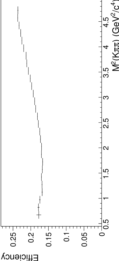
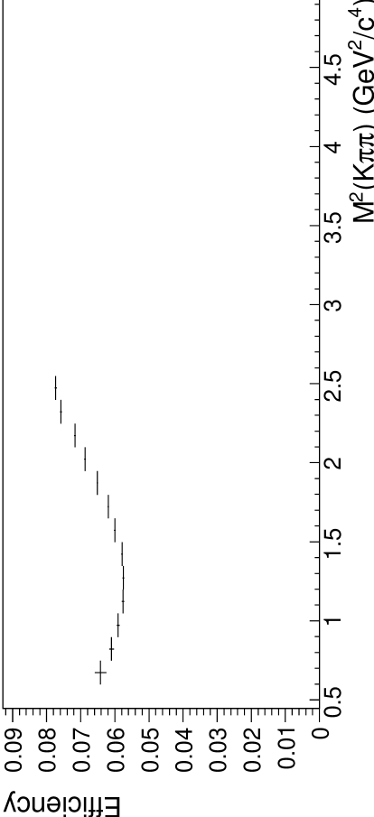
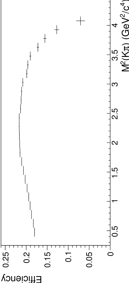
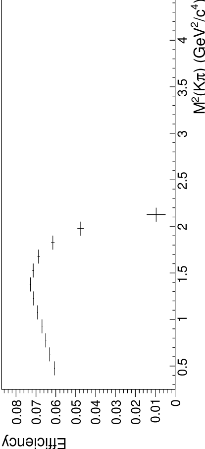
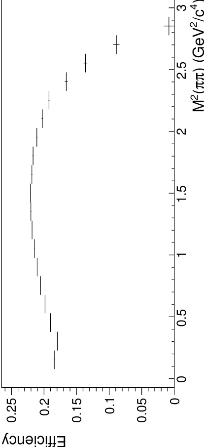
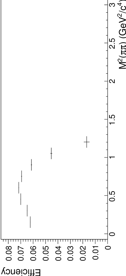
Figure 9: Dependence of the signal efficiency on the kinematic variables for $B^{+}\rightarrow J/\psi K^{+}\pi^{+}\pi^{-}$ (left) and $B^{+}\rightarrow\psi^{\prime}K^{+}\pi^{+}\pi^{-}$ (right).

    

    

    

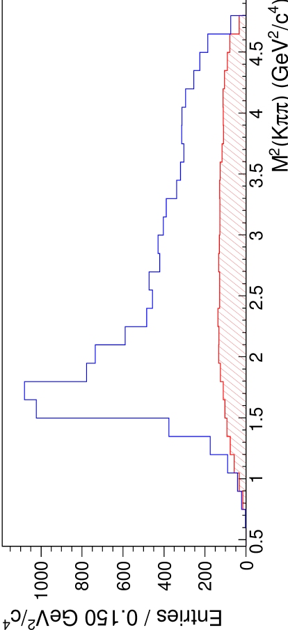
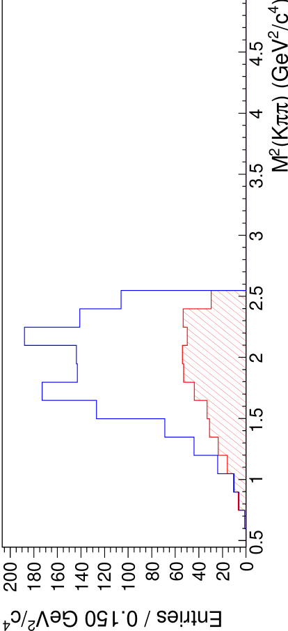
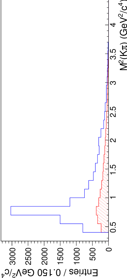
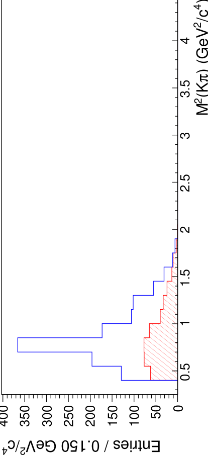
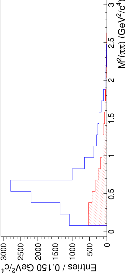
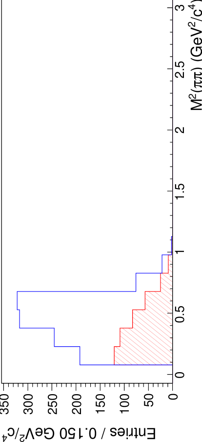
Figure 10: Data distributions of $M^{2}(K\pi\pi)$, $M^{2}(K\pi)$, and $M^{2}(\pi\pi)$ for $B^{+}\rightarrow J/\psi K^{+}\pi^{+}\pi^{-}$ (left) and $B^{+}\rightarrow\psi^{\prime}K^{+}\pi^{+}\pi^{-}$ (right) in the signal region (open histograms) and normalized sideband region (filled histograms).

This method of measuring branching fractions automatically corrects for efficiency variations over the phase space. It also makes no assumptions as to the shape of the signal in $\Delta E$.

V.1 Systematic errors

The systematic error in the branching fractions is estimated by adding in quadrature various contributions, which are assumed to be uncorrelated. Where possible, a correction is applied.

Since we use MC simulation to determine the signal efficiency in Eq. 14, any discrepancy in signal-reconstruction efficiency between data and simulation will result in a systematic error. Based on studies of the track-reconstruction efficiency, we include a systematic error of $1.0\%$ for each lepton track, $1.4\%$ for each pion track, and $1.2\%$ for each kaon track, adding linearly. Based on studies of the lepton-identification efficiency, which show that the simulation underestimates the lepton-identification efficiency, we apply a correction factor of $0.984\pm 0.019$ for each electron track and $0.962\pm 0.031$ for each muon track. Based on studies of the kaon identification efficiency, we include a systematic error of $1\%$ for $B^{+}\rightarrow J/\psi K^{+}\pi^{+}\pi^{-}$ and $2\%$ for $B^{+}\rightarrow\psi^{\prime}K^{+}\pi^{+}\pi^{-}$.

The bin size of $0.15~{}{\mathrm{GeV}}^{2}/c^{4}$ is chosen based on the dependence of the efficiency-corrected signal yield on the bin size. The error associated with this choice is taken to be the rms of the signal yield in the region between $0.1~{}{\mathrm{GeV}}^{2}/c^{4}$ and $0.2~{}{\mathrm{GeV}}^{2}/c^{4}$.

In the $\Delta E$ distributions for $B^{+}\rightarrow J/\psi K^{+}\pi^{+}\pi^{-}$ and $B^{+}\rightarrow\psi^{\prime}K^{+}\pi^{+}\pi^{-}$ nonresonant MC simulation, shown in Fig. 11, a small polynomial background can be seen under the peak. Since all the events in the MC sample include a signal decay, this “background” is made up of misreconstructed signal events. Although these events are included as signal in the efficiency calculation, they are removed by the background-subtraction procedure. The fraction of signal that is subtracted in this way is found to be $(3.75\pm 0.91)\%$ for $B^{+}\rightarrow J/\psi K^{+}\pi^{+}\pi^{-}$, and $(5.7\pm 1.2)\%$ for $B^{+}\rightarrow\psi^{\prime}K^{+}\pi^{+}\pi^{-}$. The observed branching fractions are corrected for this effect, and the associated uncertainty is included as a systematic error.

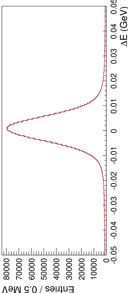
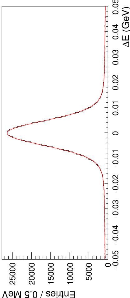
Figure 11: MC $\Delta E$ distributions for $B^{+}\rightarrow J/\psi K^{+}\pi^{+}\pi^{-}$ (top) and $B^{+}\rightarrow\psi^{\prime}K^{+}\pi^{+}\pi^{-}$ (bottom).

To determine the sideband normalization factor $f_{B}$ in Eq. 13, the data $\Delta E$ distribution is fitted as described in Sec. III.2. In this fit, the background under the signal is parametrized as a first-order polynomial. To estimate the error introduced by this assumption, a second fit is performed, parametrizing the background as a second-order polynomial. The fractional change in the signal yield is taken as a systematic error.

Since the signal and sideband regions are defined based on the results of fitting the data $\Delta E$ distribution, $\mu_{\Delta E}$ and $\sigma_{\Delta E}$ in Eqs. 6 and III.2 are varied within the fit errors.

In the MC sample used for determining the efficiency, $J/\psi$’s from the signal $B$ are forced to decay to $e^{+}e^{-}$ or $\mu^{+}\mu^{-}$, and $\psi^{\prime}$’s from the signal $B$ are forced to decay to $e^{+}e^{-}$, $\mu^{+}\mu^{-}$, or $J/\psi\pi^{+}\pi^{-}$. Thus, to obtain branching fractions for $B^{+}\rightarrow J/\psi K^{+}\pi^{+}\pi^{-}$ and $B^{+}\rightarrow\psi^{\prime}K^{+}\pi^{+}\pi^{-}$, the branching fractions measured using Eq. 14 are divided by previously-measured values pdg08 of these $J/\psi$ and $\psi^{\prime}$ decay rates. The uncertainties of these previous measurements are included as a systematic error.

Finally, the error in $N_{B}$ is $1.3\%$. Table 1 lists the components of the systematic errors.

Table 1: Components of the systematic error in the branching-fraction measurements, expressed as a percentage of the branching fraction.

Component	$B^{+}\rightarrow J/\psi K^{+}\pi^{+}\pi^{-}$	$B^{+}\rightarrow\psi^{\prime}K^{+}\pi^{+}\pi^{-}$	$B^{+}\rightarrow\psi^{\prime}K^{+}$
MC statistics	$0.18$	$0.19$	$1.12$
Tracking efficiency	$6.0$	$8.7$	$6.0$
Lepton-ID efficiency	$5.1$	$5.1$	$5.0$
Kaon-ID efficiency	$1.0$	$2.0$	$1.0$
Binning	$0.13$	$0.19$	$0.26$
Oversubtraction	$0.95$	$1.3$	$0.95$
Background shape	$1.6$	$1.3$	$0.19$
Signal/Sideband regions	$0.35$	$4.4$	$0.27$
$J/\psi$ or $\psi^{\prime}$ branching fraction	$0.71$	$1.9$	$0.67$
$N_{B}$	$1.3$	$1.3$	$1.3$

V.2 Results

The measured branching fractions are

$${\mathcal{B}}(B^{+}\rightarrow J/\psi K^{+}\pi^{+}\pi^{-}) = (7.16\pm 0.10\pm 0.60)\times 10^{-4},$$

$${\mathcal{B}}(B^{+}\rightarrow\psi^{\prime}K^{+}\pi^{+}\pi^{-}) = (4.31\pm 0.20\pm 0.50)\times 10^{-4}.$$

As a cross-check, we also measure a branching fraction for $B^{+}\rightarrow\psi^{\prime}K^{+}$, using a similar method but reversing the $\psi^{\prime}\rightarrow J/\psi\pi^{+}\pi^{-}$ veto in the reconstruction of $B^{+}\rightarrow J/\psi K^{+}\pi^{+}\pi^{-}$. This branching fraction is

$${\mathcal{B}}(B^{+}\rightarrow\psi^{\prime}K^{+})=(6.65\pm 0.17\pm 0.55)\times 10^{-4},$$

which is consistent with the previously-measured value of $(6.48\pm 0.35)\times 10^{-4}$ pdg08 .

Our $B^{+}\rightarrow J/\psi K^{+}\pi^{+}\pi^{-}$ branching-fraction measurement represents a significant improvement over previous measurements pdg08 . It is consistent with Ref. acosta:2002, but inconsistent with Ref. aubert:2005, at the $3.4$-$\sigma$ level. Our $B^{+}\rightarrow\psi^{\prime}K^{+}\pi^{+}\pi^{-}$ branching-fraction measurement is also a significant improvement over the previous measurement albrecht:1990 .

VI Amplitude analyses

To study the resonant structure of the $K^{+}\pi^{+}\pi^{-}$ final state in $B^{+}\rightarrow J/\psi K^{+}\pi^{+}\pi^{-}$ and $B^{+}\rightarrow\psi^{\prime}K^{+}\pi^{+}\pi^{-}$, we perform amplitude analyses. Using an unbinned maximum-likelihood method, we simultaneously fit the data in the three dimensions $M^{2}(K\pi\pi)$, $M^{2}(K\pi)$, and $M^{2}(\pi\pi)$.

VI.1 Fitting technique

Signal-region data are fitted by maximizing the log-likelihood function, which is given by

$$\ell(\vec{a})=\sum_{i}\ln p(\vec{x}_{i};\vec{a}),$$ (15)

where the sum is over the events in the signal region, $\vec{x}_{i}$ is the vector of coordinates for a given event (i.e., $\vec{x}\equiv[M^{2}(K\pi\pi),M^{2}(K\pi),M^{2}(\pi\pi)]$), $\vec{a}$ is the vector of parameters with respect to which $\ell$ is maximized, and $p$ is the probability-density function (PDF) that is used to model the observed distribution.

The distribution of events in the signal region is modeled as

$$p(\vec{x};\vec{a})=n_{B}\,\frac{p_{B}(\vec{x})}{\int p_{B}(\vec{x})\,d^{3}x}+n_{S}\,\frac{p_{S}(\vec{x};\vec{a})}{\int p_{S}(\vec{x};\vec{a})\,d^{3}x},$$ (16)

where $p_{B}$ and $p_{S}$ describe the observed shapes of the background and signal, respectively. The constants $n_{B}$ and $n_{S}$ are the background and signal fractions in the signal region; the former is given by Eq. 9, and the latter is $1-n_{B}$.

The observed signal distribution $p_{S}$ is expressed as

$$p_{S}(\vec{x};\vec{a})=\varepsilon(\vec{x})\phi(\vec{x})s(\vec{x};\vec{a}),$$ (17)

where $\varepsilon$ is the detector efficiency, $\phi$ is the phase-space density, and $s$ is the raw signal function.

Using nonresonant MC simulation, we have measured the detector resolution to be approximately $3$-$4~{}{\mathrm{MeV}/c^{2}}$ in each of the three coordinates $M(K\pi\pi)$, $M(K\pi)$, and $M(\pi\pi)$. Since this is smaller than the width of any resonance included in the fits, we neglect the effect of detector resolution on line shapes.

The following five sections describe the methods followed in performing the integrals of Eq. 16 and in obtaining the functions $p_{B}(\vec{x})$, $\varepsilon(\vec{x})$, $\phi(\vec{x})$, and $s(\vec{x};\vec{a})$ in Eqs. 16 and 17.

VI.2 Normalization procedure

The integrations of Eq. 16 are performed numerically, using Simpson’s rule. A step size of $0.010~{}{\mathrm{GeV}^{2}/c^{4}}$ for $B^{+}\rightarrow J/\psi K^{+}\pi^{+}\pi^{-}$ and $0.005~{}{\mathrm{GeV}^{2}/c^{4}}$ for $B^{+}\rightarrow\psi^{\prime}K^{+}\pi^{+}\pi^{-}$ is used in each dimension. The three-dimensional region of integration can be determined by noting that the minimum and maximum values of $M^{2}(K\pi\pi)$ are given by

$$M^{2}(K\pi\pi)_{\mathrm{min}} = (M_{K}+2M_{\pi})^{2},$$ (18)

$$M^{2}(K\pi\pi)_{\mathrm{max}} = (M_{B}-M_{\psi})^{2},$$ (19)

where $M_{B}$, $M_{K}$, $M_{\pi}$, and $M_{\psi}$ are the nominal values of the subscripted particles. For a given value of $M^{2}(K\pi\pi)$, the minimum and maximum values of $M^{2}(\pi\pi)$ are

$$M^{2}(\pi\pi)_{\mathrm{min}} = (2M_{\pi})^{2},$$ (20)

$$M^{2}(\pi\pi)_{\mathrm{max}} = \left(\sqrt{M^{2}(K\pi\pi)}-M_{K}\right)^{2}.$$ (21)

For given $M^{2}(K\pi\pi)$ and $M^{2}(\pi\pi)$, the minimum and maximum values of $M^{2}(K\pi)$ are

$$M^{2}(K\pi)_{\mathrm{min}}^{\mathrm{max}} = \frac{1}{2}\Biggl{[}M^{2}(K\pi\pi)+M_{K}^{2}+2M_{\pi}^{2}-M^{2}(\pi\pi)\Biggr{.}$$ (22)

$$\pm \sqrt{1-\left(2M_{\pi}/M(\pi\pi)\right)^{2}}$$

$$\times \sqrt{M^{2}(K\pi\pi)-(M_{K}+M(\pi\pi))^{2}}$$

$$\times \sqrt{M^{2}(K\pi\pi)-(M_{K}-M(\pi\pi))^{2}}\Biggl{.}\Biggr{]}.$$

Figure 12 shows the calculated kinematic boundaries for $B^{+}\rightarrow J/\psi K^{+}\pi^{+}\pi^{-}$, along with the observed distributions of sideband data, for a slice in $M^{2}(K\pi\pi)$.

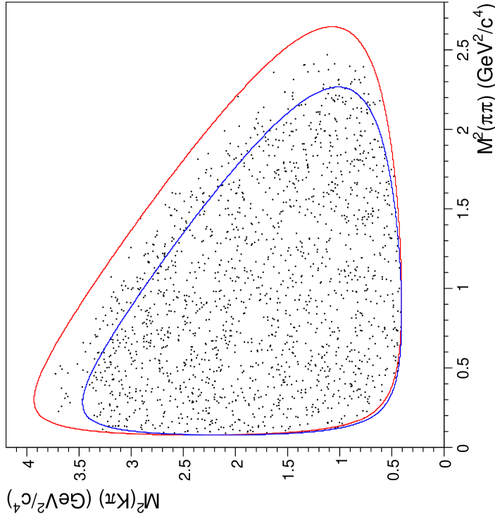
Figure 12: Scatterplot of $M^{2}(K\pi)$ versus $M^{2}(\pi\pi)$ for $M^{2}(K\pi\pi)$ between $4.0$ GeV${}^{2}/c^{4}$ and $4.5$ GeV${}^{2}/c^{4}$ in sideband data for $B^{+}\rightarrow J/\psi K^{+}\pi^{+}\pi^{-}$. Blue and red curves show the calculated boundaries corresponding to the low and high edge, respectively, of the plotted $M^{2}(K\pi\pi)$ region.

Events that do not fall within the calculated boundaries are excluded from the fits. Because of the coordinate transformations of Sec. IV, such events are rare: $36$ of the $12913$ sideband events and $3$ of the $10594$ signal-region events for $B^{+}\rightarrow J/\psi K^{+}\pi^{+}\pi^{-}$, and $3$ of the $2230$ sideband events and none of the $1176$ signal-region events for $B^{+}\rightarrow\psi^{\prime}K^{+}\pi^{+}\pi^{-}$ fall outside the boundaries.

VI.3 Background functions

To determine the three-dimensional shape of the background in the signal region (i.e., $p_{B}(\vec{x})$ in Eq. 16), an unbinned maximum-likelihood fit is performed on the sideband-region data. The log-likelihood function to maximize is given in this case by

$$\ell_{B}(\vec{a}_{B})=\sum_{j}\ln\frac{p_{B}(\vec{x}_{j};\vec{a}_{B})}{\int p_{B}(\vec{x};\vec{a}_{B})\,d^{3}x},$$ (23)

where the sum is over the events in the sideband region. The maximization is performed by varying the parameters $\vec{a}_{B}$, which are then fixed at their optimal values in fitting the signal region.

The background is modeled as the sum of a combinatorial term and a set of noninterfering resonances. For $B^{+}\rightarrow J/\psi K^{+}\pi^{+}\pi^{-}$,

$$p_{B}(\vec{x};\vec{a}_{B})=\Biggl{[}\,\sum_{i=0}^{5}a_{xi}T_{i}(x)\,\Biggr{]}$$ (24)

$${}\times\Biggl{[}\,\sum_{j=0}^{1}a_{yj}T_{j}(y)\,\Biggr{]}\times\Biggl{[}\,\sum_{k=0}^{2}a_{zk}T_{k}(z)\,\Biggr{]}$$

$${}+e^{-2x}\Bigl{[}\Bigr{.}a_{K^{*}(892)}BW_{K^{*}(892)}(y)+a_{\rho}BW_{\rho}(z)$$

$${~{}~{}~{}~{}~{}~{}~{}~{}~{}~{}}+a_{D}G_{D}(y)+a_{K_{S}}G_{K_{S}}(z)\Bigl{.}\Bigr{]},$$

and for $B^{+}\rightarrow\psi^{\prime}K^{+}\pi^{+}\pi^{-}$,

$$p_{B}(\vec{x};\vec{a}_{B})=\Biggl{[}\,\sum_{i=0}^{3}a_{xi}T_{i}(x)\,\Biggr{]}$$ (25)

$${}+e^{-2x}\Bigl{[}\Bigr{.}a_{K^{*}(892)}BW_{K^{*}(892)}(y)+a_{\rho}BW_{\rho}(z)\Bigl{.}\Bigr{]}.$$

In Eqs. 24 and 25, $T_{n}$ represents an $n$th-order Chebyshev polynomial. The variables $x$, $y$, and $z$ stand for $M^{2}(K\pi\pi)$, $M^{2}(K\pi)$, and $M^{2}(\pi\pi)$, respectively, and are defined over the intervals

$$x_{\mathrm{min}} =(M_{K}+2M_{\pi})^{2}\,, x_{\mathrm{max}} =(M_{B}-M_{\psi})^{2}\,,$$

$$y_{\mathrm{min}} =(M_{K}+M_{\pi})^{2}\,, y_{\mathrm{max}} =(M_{B}-M_{\psi}-M_{\pi})^{2}\,,$$

$$z_{\mathrm{min}} =(2M_{\pi})^{2}\,, z_{\mathrm{max}} =(M_{B}-M_{\psi}-M_{K})^{2}\,.$$

The peak functions $BW_{K^{*}(892)}$, $G_{D}$, $G_{K_{S}}$, and $BW_{\rho}$ are obtained as described in Sec. IV. Each peak function $P(\vec{x})$ is normalized over the kinematically-allowed phase space to satisfy

$$1=\int e^{-2x}P(\vec{x})d^{3}x.$$ (26)

The factor of $e^{-2x}$ that modulates the peak functions was found empirically to produce a good fit to the sideband data.

Table 2 lists the fitted parameters of the background functions. The statistical error in each parameter is defined as the change in that parameter required to reduce the log likelihood by $1/2$. The fitted functions, normalized to the total number of events in the fit, are shown projected onto the three axes along with the sideband data in Fig. 13. Figures 14 and 15 show $M^{2}(K\pi)$ and $M^{2}(\pi\pi)$ projections for slices in $M^{2}(K\pi\pi)$.

Table 2: Fitted values of the background-function parameters (Eqs. 24 and 25).

Parameter	$B^{+}\rightarrow J/\psi K^{+}\pi^{+}\pi^{-}$		$B^{+}\rightarrow\psi^{\prime}K^{+}\pi^{+}\pi^{-}$
$a_{x0}$	$1.0$ (fixed)		$1.0$ (fixed)
$a_{x1}$	$-1.5901$$~{}\pm~{}$	$0.0048$	$-1.238$$~{}\pm~{}$	$0.036$
$a_{x2}$	$0.9423$$~{}\pm~{}$	$0.0086$	$0.480$$~{}\pm~{}$	$0.045$
$a_{x3}$	$-0.4737$$~{}\pm~{}$	$0.0087$	$-0.221$$~{}\pm~{}$	$0.021$
$a_{x4}$	$0.1778$$~{}\pm~{}$	$0.0067$
$a_{x5}$	$-0.0488$$~{}\pm~{}$	$0.0033$
$a_{y0}$	$1.0$ (fixed)
$a_{y1}$	$0.088$$~{}\pm~{}$	$0.021$
$a_{z0}$	$1.0$ (fixed)
$a_{z1}$	$-0.022$$~{}\pm~{}$	$0.022$
$a_{z2}$	$0.129$$~{}\pm~{}$	$0.018$
$a_{K^{*}(892)}$	$0.0353$$~{}\pm~{}$	$0.0065$	$0.0161$$~{}\pm~{}$	$0.0062$
$a_{D}$	$0.0007$$~{}\pm~{}$	$0.0011$
$a_{K_{S}}$	$0.0061$$~{}\pm~{}$	$0.0023$
$a_{\rho}$	$0.086$$~{}\pm~{}$	$0.012$	$0.0352$$~{}\pm~{}$	$0.0099$

    

    

    

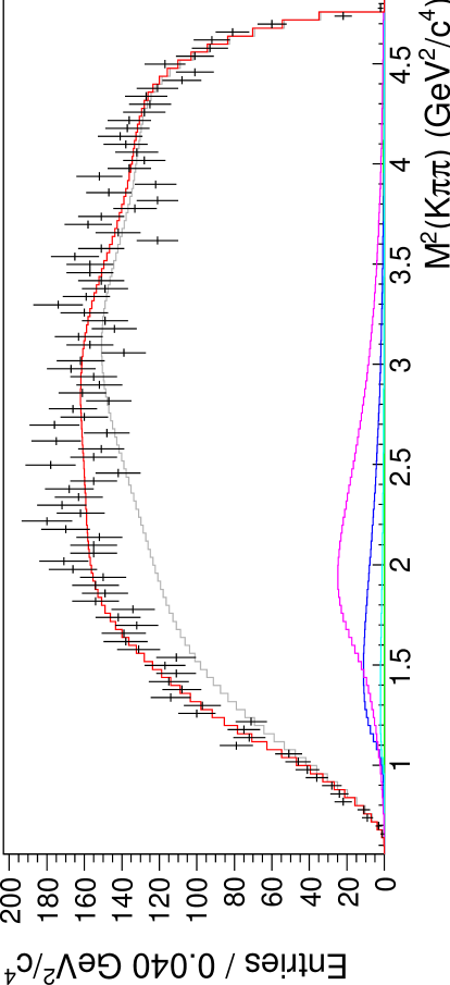
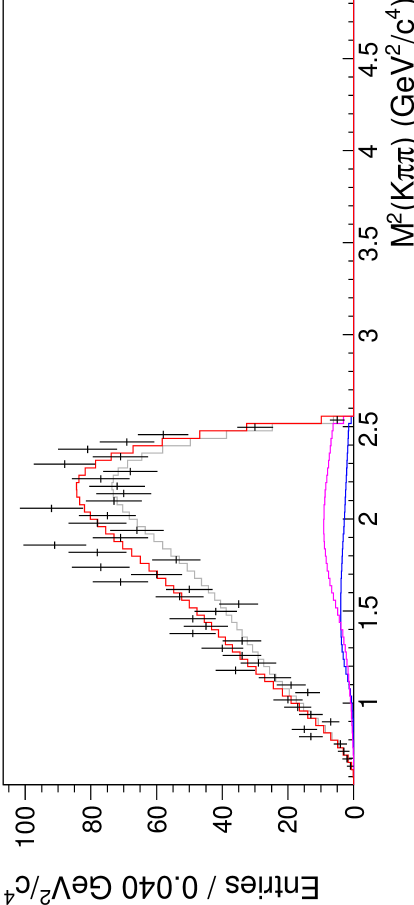
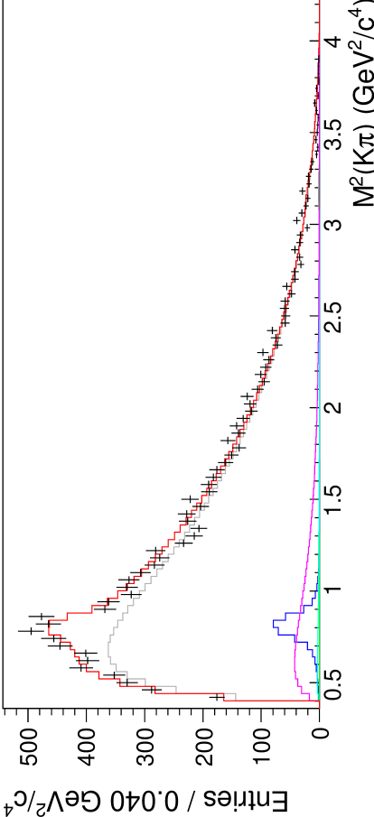
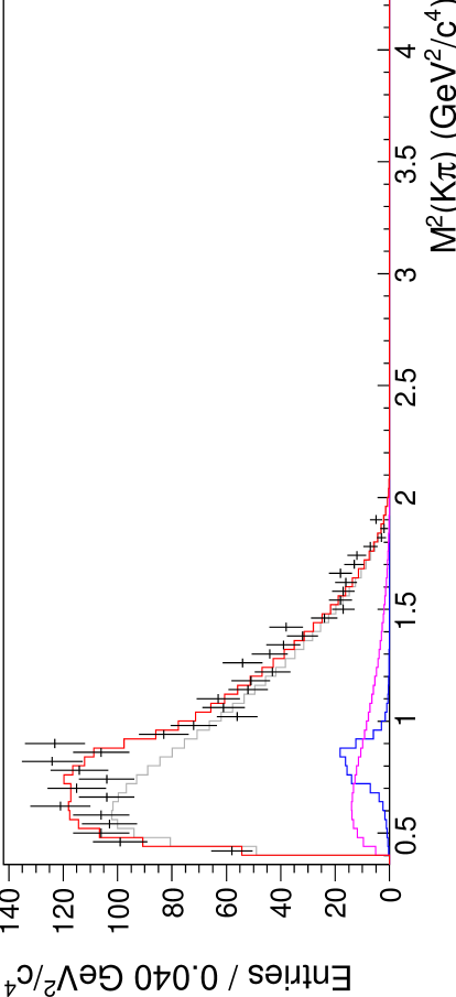
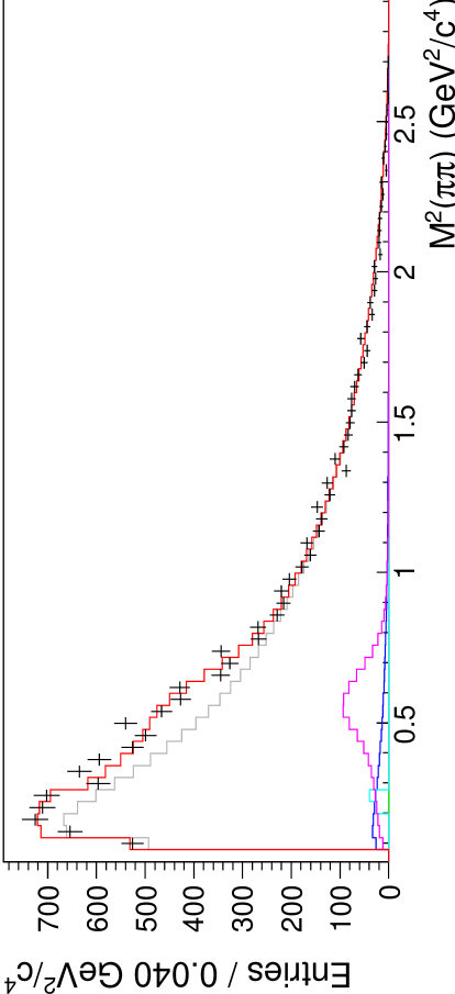
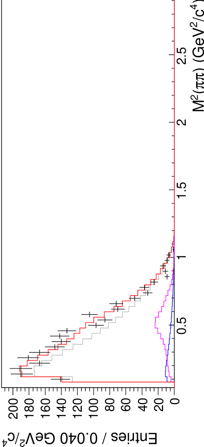
Figure 13: Results of sideband fits for $B^{+}\rightarrow J/\psi K^{+}\pi^{+}\pi^{-}$ (left) and $B^{+}\rightarrow\psi^{\prime}K^{+}\pi^{+}\pi^{-}$ (right). Data (points) and fits (histograms) are shown projected onto the three axes. The red histograms show the overall background functions. The combinatorial components are shown in gray, while the $K^{*}(892)$, $\rho$, $K_{S}$ and $D$ backgrounds are shown in blue, magenta, cyan, and green, respectively. The $K^{*}(892)$ and $\rho$ peaks are broader in $B^{+}\rightarrow\psi^{\prime}K^{+}\pi^{+}\pi^{-}$ than in $B^{+}\rightarrow J/\psi K^{+}\pi^{+}\pi^{-}$ because the distortion shown in Fig. 8 is larger in the former mode.

    

    

    

    

    

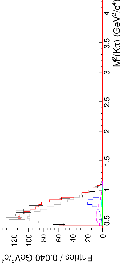
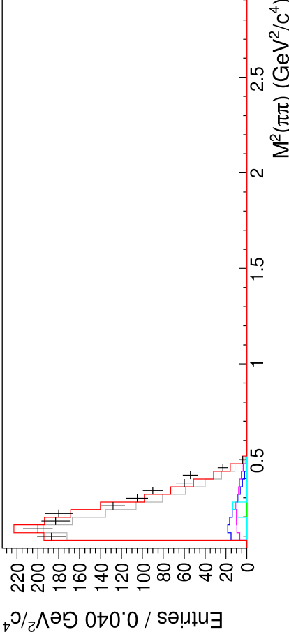
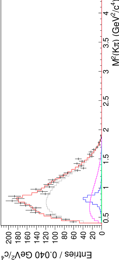
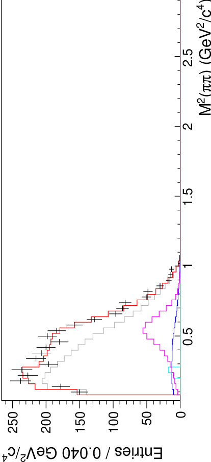
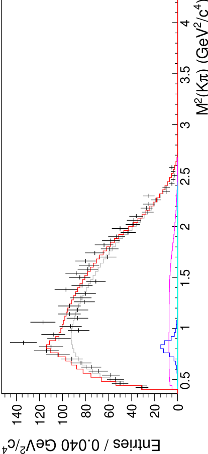
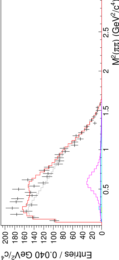
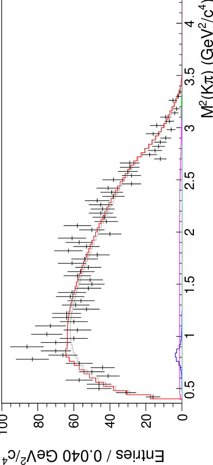
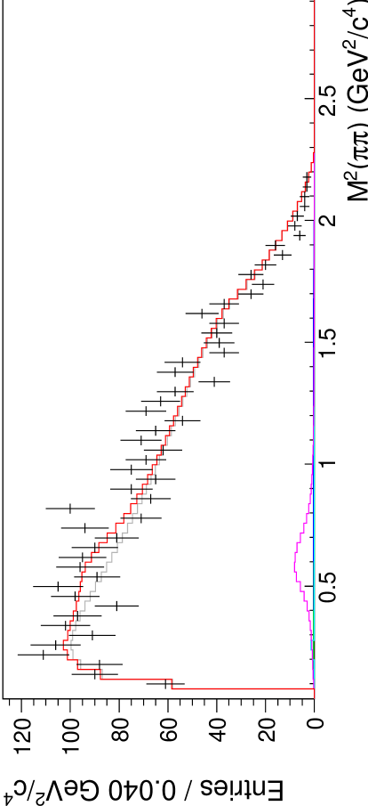
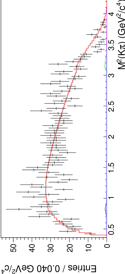
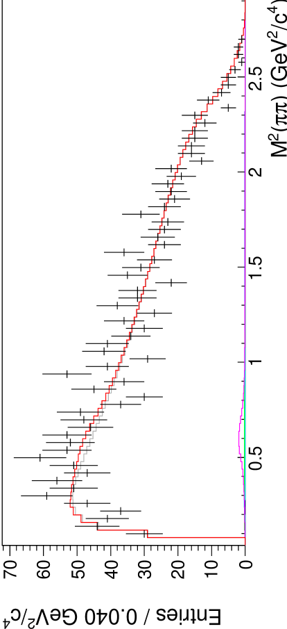
Figure 14: $B^{+}\rightarrow J/\psi K^{+}\pi^{+}\pi^{-}$ sideband data (points) and fit results (histograms) for slices in $M^{2}(K\pi\pi)$. The fit components are color coded as in Fig. 13.

    

    

    

    

    

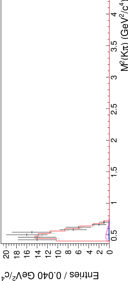
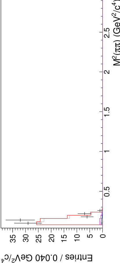
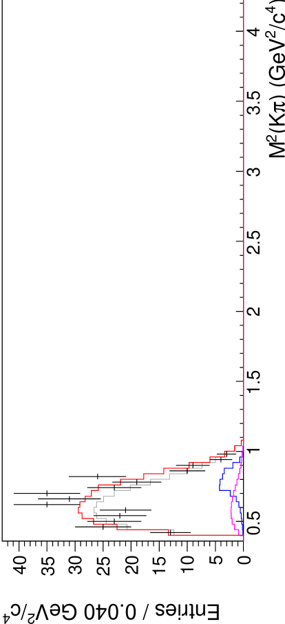
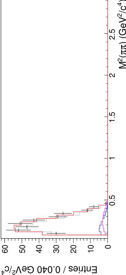
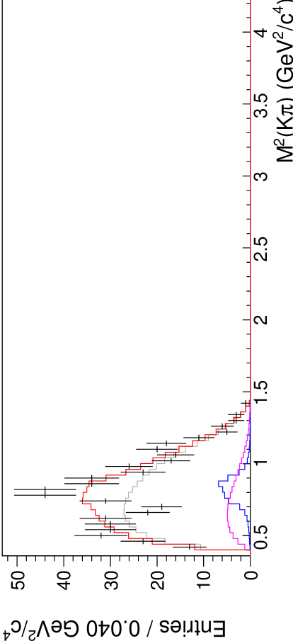
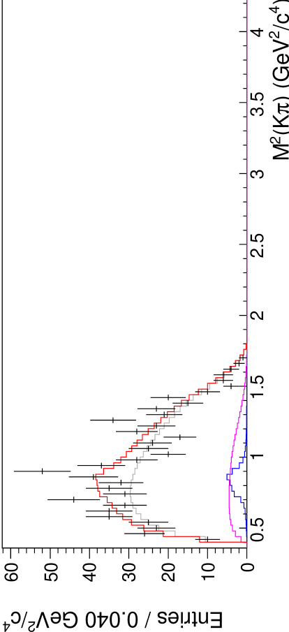
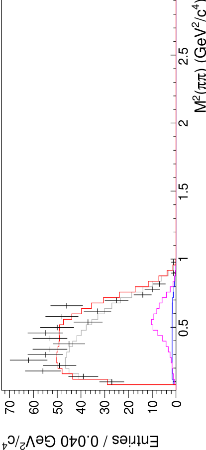
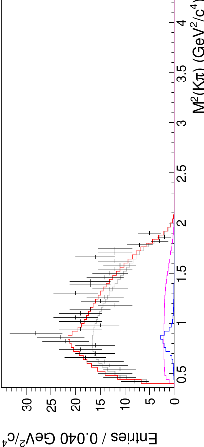
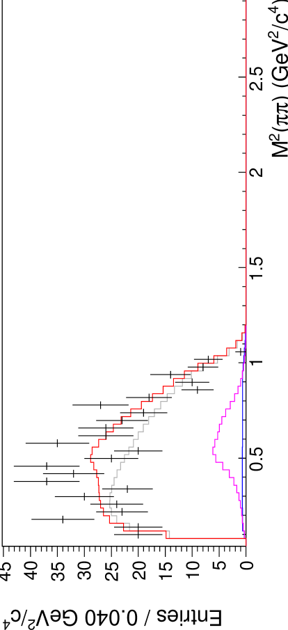
Figure 15: $B^{+}\rightarrow\psi^{\prime}K^{+}\pi^{+}\pi^{-}$ sideband data (points) and fit results (histograms) for slices in $M^{2}(K\pi\pi)$. The fit components are color coded as in Fig. 13.

As a measure of goodness of fit, a $\chi^{2}$ variable is calculated by distributing the data into cubic bins that are $0.1~{}{\mathrm{GeV}}/c^{2}$ wide on each side. The normalized PDF, with the parameters set to their best-fit values, is integrated over each bin and multiplied by the total number of events in the fit to determine the number of events expected in the bin. Adjacent bins are combined until each bin has at least $6$ data events. A $\chi^{2}$ variable for the multinomial distribution is then calculated as baker:1984

$$\chi^{2}=2\sum_{i}^{N_{\mathrm{bins}}}n_{i}\ln\left(\frac{n_{i}}{p_{i}}\right),$$ (27)

where $N_{\mathrm{bins}}$ is the total number of bins used, $n_{i}$ is the number of observed events in a given bin, and $p_{i}$ is the number expected in that bin based on the PDF.

If the expected distribution $p_{i}$ were obtained by a binned maximum-likelihood fit of the data distribution $n_{i}$, the number of degrees of freedom associated with this $\chi^{2}$ would be reduced by the number of fit parameters $N_{\mathrm{par}}$ and would be given by $N_{\mathrm{DOF}}=N_{\mathrm{bins}}-N_{\mathrm{par}}-1$. If, on the other hand, the two distributions were not correlated by a fit, the number of degrees of freedom would be $N_{\mathrm{DOF}}=N_{\mathrm{bins}}-1$. Since, in this case, the distributions are related by an unbinned maximum-likelihood fit, the true $N_{\mathrm{DOF}}$ can be expected to lie between these extremes kopp:2001 .

For the $B^{+}\rightarrow J/\psi K^{+}\pi^{+}\pi^{-}$ sideband-data fit, $\ell_{B}=-21484.6$, while $\chi^{2}=1709.5$ with $N_{\mathrm{bins}}=1707$ and $N_{\mathrm{par}}=12$. For the $B^{+}\rightarrow\psi^{\prime}K^{+}\pi^{+}\pi^{-}$ sideband-data fit, $\ell_{B}=822.7$, while $\chi^{2}=286.8$ with $N_{\mathrm{bins}}=294$ and $N_{\mathrm{par}}=5$.

VI.4 Efficiency functions

The dependence of the detector efficiency on the kinematic variables (i.e., $\varepsilon(\vec{x})$ in Eq. 17) is obtained for three-dimensional bins, $0.15~{}{\mathrm{GeV}}^{2}/c^{4}$-wide on each side, using nonresonant signal-MC simulation as described in Sec. V and illustrated in Fig. 9. The function is implemented as a lookup table: the efficiency for a given data point is the efficiency in the corresponding bin.

VI.5 Phase-space densities

Four-body phase-space densities (i.e., $\phi(\vec{x})$ in Eq. 17) for $B^{+}\rightarrow J/\psi K^{+}\pi^{+}\pi^{-}$ and $B^{+}\rightarrow\psi^{\prime}K^{+}\pi^{+}\pi^{-}$ are obtained by using GENBOD genbod to generate final-state-particle four-momenta that are weighted by the density of states in phase space james:1968u . For each decay mode, $10^{8}$ events are generated. Event phase-space weights are distributed into cubic bins in $M^{2}(K\pi\pi)$, $M^{2}(K\pi)$, and $M^{2}(\pi\pi)$, with a bin width of $0.02~{}{\mathrm{GeV}}^{2}/c^{4}$. The phase-space density is implemented as a lookup table: the value of $\phi(\vec{x})$ for a given data point is the total phase-space weight in the corresponding bin. In Fig. 16, the three-dimensional histogram of phase-space weights is projected onto the three axes, showing the distribution that signal events would have in the absence of resonant effects.

Figure 16 does not indicate the functional form of $\phi(\vec{x})$, since the projection onto a single dimension effectively integrates over the other two dimensions, and the region of integration is the complicated one described in Sec. VI.2. In Fig. 17, the same projections are performed over a narrow slice in each of the other two dimensions, to illustrate the dependence of the function $\phi(\vec{x})$ on each variable.

    

    

    

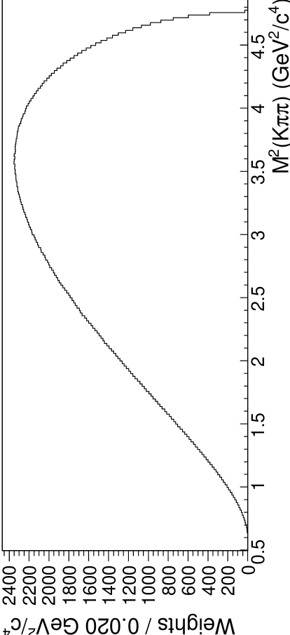
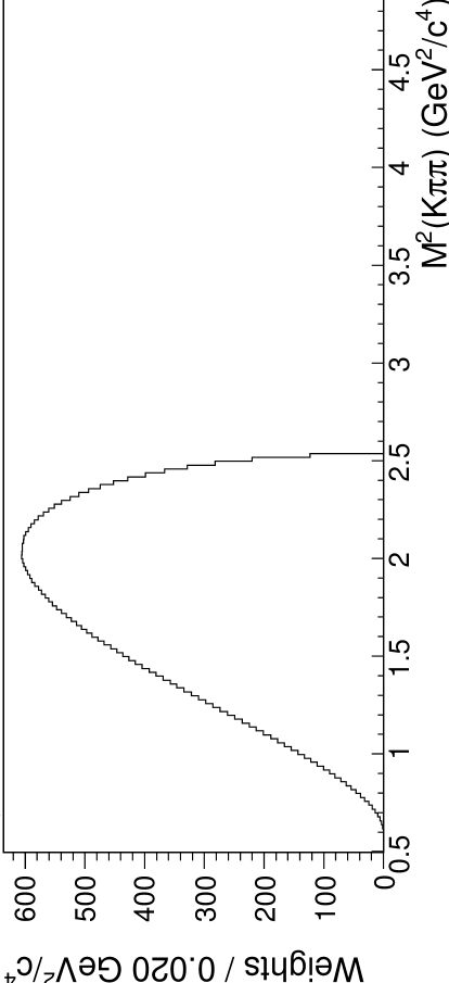
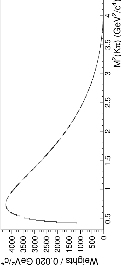
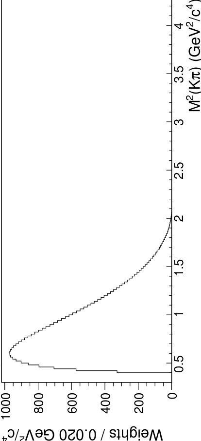
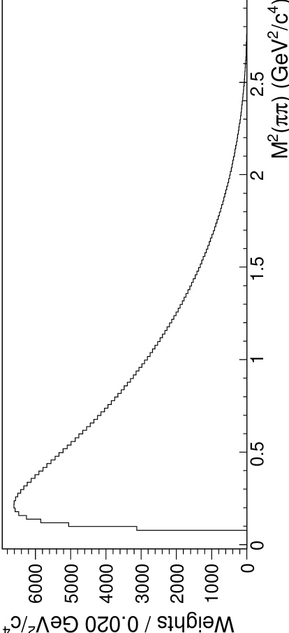
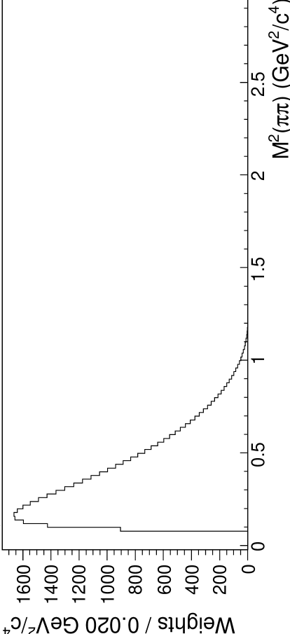
Figure 16: Projections of the three-dimensional histogram of phase-space weights onto the three axes for $B^{+}\rightarrow J/\psi K^{+}\pi^{+}\pi^{-}$ (left) and $B^{+}\rightarrow\psi^{\prime}K^{+}\pi^{+}\pi^{-}$ (right).

    

    

    

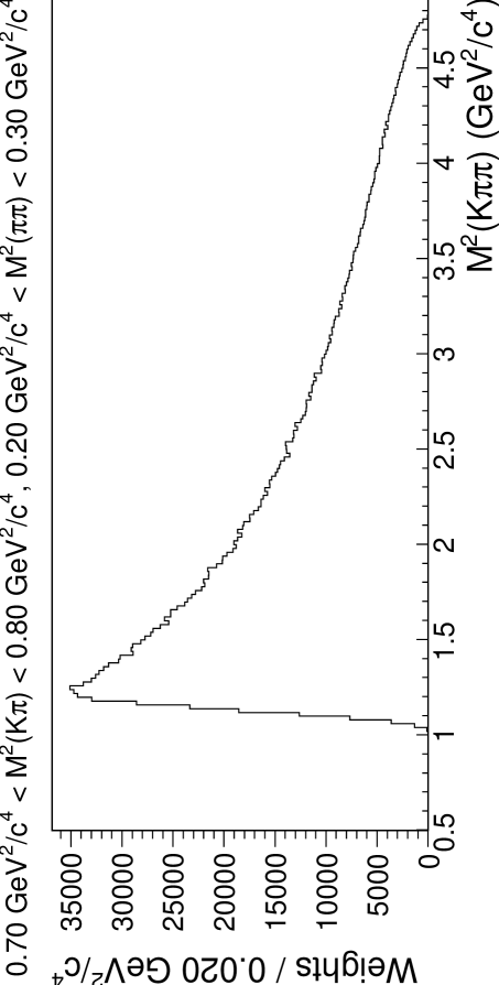
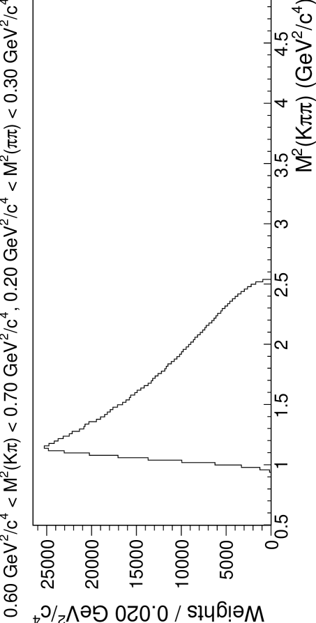
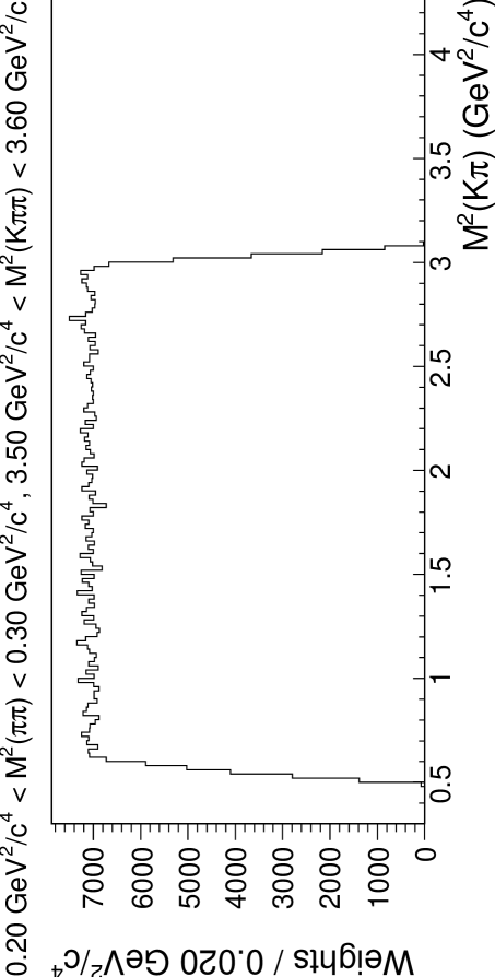
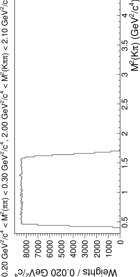
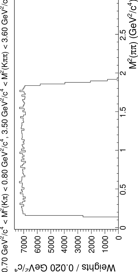
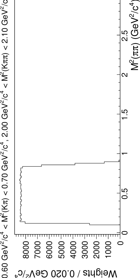
Figure 17: Phase-space densities for selected regions, as a function of $M^{2}(K\pi\pi)$, $M^{2}(K\pi)$, and $M^{2}(\pi\pi)$, for $B^{+}\rightarrow J/\psi K^{+}\pi^{+}\pi^{-}$ (left) and $B^{+}\rightarrow\psi^{\prime}K^{+}\pi^{+}\pi^{-}$ (right). In each case, the region selected is indicated above the plot.

VI.6 Signal functions

The $K^{+}\pi^{+}\pi^{-}$ final state is modeled as a nonresonant signal plus a superposition of initial-state resonances $R_{1}$. The latter are assumed to decay through intermediate-state resonances $R_{2}$ as $R_{1}\rightarrow aR_{2}$, $R_{2}\rightarrow bc$, where $a$, $b$, and $c$ are the final-state particles. Specifically, the function $s(\vec{x};\vec{a})$ of Eq. 17 is expressed as

$$s(\vec{x};\vec{a})\equiv s(\vec{x};a_{k})$$ (28)

$$= \left|a_{nr}A_{nr}(\vec{x})\right|^{2}+\sum_{J_{1}}\left|\sum_{J_{2}}a_{J_{1}J_{2}}A_{J_{1}J_{2}}(\vec{x})\right|^{2}.$$

Here, $J_{1}$ and $J_{2}$ stand for the spin-parity ($J^{P}$) of $R_{1}$ and $R_{2}$, respectively. Resonances with different $J_{1}$ are added incoherently, while those with the same $J_{1}$ are added coherently. The parameters varied in the fit are the complex coefficients $a_{nr}$ and $a_{J_{1}J_{2}}$, collectively referred to as $a_{k}$. While the nonresonant signal is assumed to be constant over the phase space,

$$A_{nr}(\vec{x})=1,$$ (29)

the resonant decay amplitudes $A_{J_{1}J_{2}}$ are expressed as

$$A_{J_{1}J_{2}}(\vec{x}) = \alpha_{J_{1}J_{2}}$$ (30)

$$\times \frac{\sqrt{M_{R_{1}}\Gamma_{R_{1}}}}{M_{R_{1}}^{2}-m_{abc}^{2}-iM_{R_{1}}\Gamma_{R_{1}}}$$

$$\times \frac{\sqrt{M_{R_{2}}\Gamma_{R_{2}}(m_{bc})}}{M_{R_{2}}^{2}-m_{bc}^{2}-iM_{R_{2}}\Gamma_{R_{2}}(m_{bc})},$$

where $\Gamma_{R_{2}}(m_{bc})$ is the mass-dependent width

$$\Gamma_{R_{2}}(m_{bc})=\Gamma_{R_{2}}\left(\frac{q}{q_{0}}\right)^{2J_{2}+1}\left(\frac{M_{R_{2}}}{m_{bc}}\right)F_{R}^{2},$$ (31)

and $F_{R}$ is the Blatt-Weisskopf barrier factor

$$F_{R} =1 {\text{ for }}J_{2}=0,$$

$$=\frac{\sqrt{1+R^{2}q_{0}^{2}}}{\sqrt{1+R^{2}q^{2}}} {\text{ for }}J_{2}=1,$$ (32)

$$=\frac{\sqrt{9+3R^{2}q_{0}^{2}+R^{4}q_{0}^{4}}}{\sqrt{9+3R^{2}q^{2}+R^{4}q^{4}}} {\text{ for }}J_{2}=2.$$

The meson radial parameter $R$ is set to $1.5~{}({\mathrm{GeV}}/c)^{-1}$. The function $\alpha_{J_{1}J_{2}}$ describes the spin-dependent angular distribution of the final state and is shown for various combinations of $J_{1}$ and $J_{2}$ in Table 3. Resonances with spin greater than two are not included in the fitting model. In cases where there is more than one covariant spin amplitude, only the lowest spin is included.

Table 3: Angular distribution of the $K^{+}\pi^{+}\pi^{-}$ final state for various combinations of initial and intermediate-state spin parities. See Ref. filippini:1995, for derivation and conditions of applicability.

$J_{1}$	$J_{2}$	$\alpha_{J_{1}J_{2}}$
	$0^{+}$
Any	$0^{-}$	$1$
$0^{+}$	$1^{+}$
$0^{-}$	$1^{-}$	$(1+z^{2})\cos^{2}\theta$
$1^{+}$	$1^{-}$
$1^{-}$	$1^{+}$	$1+z^{2}\cos^{2}\theta$
$1^{+}$	$1^{+}$
$1^{-}$	$1^{-}$	$1-\cos^{2}\theta$
$1^{+}$	$2^{+}$	$(1+z^{2})$
$1^{-}$	$2^{-}$	${}\times\left[1+3\cos^{2}\theta+9z^{2}(\cos^{2}\theta-1/3)^{2}\right]$
$2^{+}$	$1^{+}$
$2^{-}$	$1^{-}$	$3+(1+4z^{2})\cos^{2}\theta$
$2^{+}$	$1^{-}$
$2^{-}$	$1^{+}$	$1-\cos^{2}\theta$
$2^{+}$	$2^{+}$	$1+z^{2}/9+(z^{2}/3-1)\cos^{2}\theta$
$2^{-}$	$2^{-}$	${}-z^{2}(\cos^{2}\theta-1/3)^{2}$
$2^{+}$	$2^{-}$
$2^{-}$	$2^{+}$	$1+z^{2}/3+z^{2}\cos^{2}\theta+z^{4}(\cos^{2}\theta-1/3)^{2}$

In Eqs. 30-VI.6 and Table 3, the nominal masses of the resonances $R_{1}$ and $R_{2}$ are denoted by $M_{R_{1}}$ and $M_{R_{2}}$, and the nominal widths by $\Gamma_{R_{1}}$ and $\Gamma_{R_{2}}$. The angle $\theta$ is between $a$ and $b$ in the $bc$ rest frame and can be expressed as

$$\cos\theta=\frac{m_{bc}}{4pqm_{abc}}$$ (33)

$$\times \left[m_{ac}^{2}-m_{ab}^{2}+\frac{(m_{abc}^{2}-m_{a}^{2})(m_{b}^{2}-m_{c}^{2})}{m_{bc}^{2}}\right].$$

The variable $z$ is given by

$$z=p/m_{abc}.$$ (34)

The breakup momentum $p$ is the momentum of $a$ or $bc$ in the $abc$ rest frame:

$$p^{2}=\frac{(m_{abc}^{2}-(m_{a}+m_{bc})^{2})(m_{abc}^{2}-(m_{a}-m_{bc})^{2})}{4m_{abc}^{2}},$$ (35)

while $q$ is the momentum of $b$ or $c$ in the $bc$ rest frame:

$$q^{2}=\frac{(m_{bc}^{2}-(m_{b}+m_{c})^{2})(m_{bc}^{2}-(m_{b}-m_{c})^{2})}{4m_{bc}^{2}},$$ (36)

where the constant $q_{0}$ is the value of $q$ evaluated at $m_{bc}=M_{R_{2}}$.

Since the components of the signal function are not individually normalized, it is not meaningful to compare the moduli of the complex coefficients $a_{k}$ in Eq. 28. A decay fraction is therefore calculated for each component by integrating the component over the kinematically-allowed region and dividing by the integral of the full signal function

$$f_{k}=\frac{\int\phi(\vec{x})|a_{k}A_{k}(\vec{x})|^{2}d^{3}x}{\int\phi(\vec{x})s(\vec{x};\vec{a})d^{3}x}.$$ (37)

The integrations in Eq. 37 are performed as described in Sec. VI.2. Because of interference effects, decay fractions for a given final state will not, in general, add up to unity.

VI.7 Statistical errors

As with the sideband-region fits, the statistical uncertainties in the fit parameters (i.e., moduli and phases) are determined by the fitter: the error in a given parameter is the change in that parameter that reduces the log likelihood by $1/2$. The statistical uncertainties in the decay fractions, on the other hand, are more complicated. Since a given decay fraction involves the integral of the full signal function, the error in a single decay fraction incorporates the errors in all of the parameters. To determine the statistical errors in the decay fractions, $1000$ sets of correlated signal-function parameters are drawn from Gaussian distributions using the fitted parameter values and the error matrix. Decay fractions are calculated for each set of generated parameters. The rms of the resulting distribution provides an estimate of the statistical error in the decay fraction.

VI.8 Systematic errors

Several sources of systematic error are considered, as described below. They are added in quadrature to obtain the systematic errors reported in Sec. VI.9.

VI.8.1 Background parametrization

A possible source of systematic error in the fits is the fixed background fraction $n_{B}$ in Eq. 16. While the error in $n_{B}$ is small, the correction for the oversubtraction, described in Sec. V.1, lowers $n_{B}$ by $10.8\%$ for $B^{+}\rightarrow J/\psi K^{+}\pi^{+}\pi^{-}$ and by $11.4\%$ for $B^{+}\rightarrow\psi^{\prime}K^{+}\pi^{+}\pi^{-}$. The systematic error associated with this correction is estimated conservatively as the change in each parameter when the fits are performed with the uncorrected values of $n_{B}$.

There may be an additional systematic error if the background in the signal region is not correctly parametrized by the shape determined by fitting the sidebands. As noted in Sec. IV, generic-MC studies suggest that not enough of the $K_{S}^{0}$ and $\rho$ background peaks are removed by the sideband subtraction. To estimate this error, a fit is performed in which the coefficients of the background peaks in Eqs. 24 and 25 are doubled.

VI.8.2 Efficiency

To estimate the error introduced by binning the efficiency information, the fits are repeated using bin sizes of $0.10~{}{{\mathrm{GeV}}^{2}/c^{4}}$ and $0.20~{}{{\mathrm{GeV}}^{2}/c^{4}}$ for the efficiency. The average absolute change in each parameter is the estimate of the error.

Another possible source of error is that the MC simulation may not faithfully reproduce the detector efficiency for low-momentum particles. To test for such an effect, two additional fits are performed. In the first fit, only charged particles with a momentum greater than $200~{}{\mathrm{MeV}}/c$ are included. In the second fit, the $|dr|$ and $|dz|$ requirements described in Sec. III are loosened from $0.4~{}{\mathrm{cm}}$ to $0.8~{}{\mathrm{cm}}$, and from $1.5~{}{\mathrm{cm}}$ to $3.0~{}{\mathrm{cm}}$, respectively. The changes in each parameter observed in these two fits are added in quadrature to obtain an estimate of the error due to inaccuracies in the efficiency estimation.

Using only the three variables $M^{2}(K\pi\pi)$, $M^{2}(K\pi)$, and $M^{2}(\pi\pi)$ in this analysis is equivalent to integrating over variables that describe the relative momentum of the $J/\psi$ or $\psi^{\prime}$ with respect to the $K^{+}\pi^{+}\pi^{-}$ system. In this integration, the terms corresponding to $K^{+}\pi^{+}\pi^{-}$ states with different initial-state spin-parity cancel out, producing Eq. 28. This cancellation, however, is exact only if the detector efficiency is flat over the extra variables. To determine the effect of neglecting these variables, an additional set of fits is performed, in which the efficiency in Eq. 17 is calculated as a function of the two angles between the $J/\psi$ or $\psi^{\prime}$ and the $K^{+}\pi^{+}\pi^{-}$ system, rather than $M^{2}(K\pi\pi)$, $M^{2}(K\pi)$, and $M^{2}(\pi\pi)$. The resulting fitted parameters are compared to those obtained by a fit in which the efficiency is held constant. The absolute change in each parameter is found to be small (less than $15\%$ of the statistical error) and is included in the systematic error.

VI.8.3 Integration step size

To estimate the error introduced by the finite step size used in the numerical integrals of Secs. IV and VI.2, the fits are repeated, using a step size of $0.005~{}{\mathrm{GeV}^{2}/c^{4}}$ for $B^{+}\rightarrow J/\psi K^{+}\pi^{+}\pi^{-}$ and $0.010~{}{\mathrm{GeV}^{2}/c^{4}}$ for $B^{+}\rightarrow\psi^{\prime}K^{+}\pi^{+}\pi^{-}$. The change in each parameter is an estimate of the uncertainty associated with the numerical integration.

VI.8.4 Modeling of the signal

The masses and widths of the resonances included in the fits are listed in Table 4. To estimate the systematic error associated with the uncertainties in these quantities, the fits are repeated, varying each fixed quantity within its errors. For each mass or width, the average absolute change in each parameter is recorded. These average changes are then added in quadrature.

Table 4: Masses, widths, and spin-parity values of the resonances included in the fits. With the exception of the $K(1600)$ parameters (discussed in Sec. VI.10.3), all values are from pdg08 .

	Mass		Width
Resonance	(${\mathrm{MeV}}/c^{2}$)		(${\mathrm{MeV}}/c^{2}$)		$J^{P}$
$\rho^{0}$	$775.49$$~{}\pm~{}$	$0.34$	$146.2$$~{}\pm~{}$	$0.7$	$1^{-}$
$\omega$	$782.65$$~{}\pm~{}$	$0.12$	$8.49$$~{}\pm~{}$	$0.08$	$1^{-}$
$f_{0}(980)^{0}$	$980$$~{}\pm~{}$	$10$	$50$$~{}\pm~{}$	${}^{50}_{10}$	$0^{+}$
$f_{2}(1270)^{0}$	$1275.1$$~{}\pm~{}$	$1.2$	$185.1$$~{}\pm~{}$	${}^{2.9}_{2.4}$	$0^{+}$
$K^{*}(892)^{0}$	$896.00$$~{}\pm~{}$	$0.25$	$50.3$$~{}\pm~{}$	$0.6$	$1^{-}$
$K_{1}(1270)^{+}$	$1272$$~{}\pm~{}$	$7$	$90$$~{}\pm~{}$	$20$	$1^{+}$
$K_{1}(1400)^{+}$	$1403$$~{}\pm~{}$	$7$	$174$$~{}\pm~{}$	$13$	$1^{+}$
$K^{*}(1410)^{+}$	$1414$$~{}\pm~{}$	$15$	$232$$~{}\pm~{}$	$21$	$1^{-}$
$K_{0}^{*}(1430)^{+}$	$1425$$~{}\pm~{}$	$50$	$270$$~{}\pm~{}$	$80$	$0^{+}$
$K_{2}^{*}(1430)^{+}$	$1425.6$$~{}\pm~{}$	$1.5$	$98.5$$~{}\pm~{}$	$2.7$	$2^{+}$
$K_{2}^{*}(1430)^{0}$	$1432.4$$~{}\pm~{}$	$1.3$	$109$$~{}\pm~{}$	$5$	$2^{+}$
$K(1600)^{+}$	$1605$$~{}\pm~{}$	$15$	$115$$~{}\pm~{}$	$15$	$2^{-}$
$K^{*}(1680)^{+}$	$1717$$~{}\pm~{}$	$27$	$322$$~{}\pm~{}$	$110$	$1^{-}$
$K_{2}(1770)^{+}$	$1773$$~{}\pm~{}$	$8$	$186$$~{}\pm~{}$	$14$	$2^{-}$
$K_{2}^{*}(1980)^{+}$	$1973$$~{}\pm~{}$	$26$	$373$$~{}\pm~{}$	$68$	$2^{+}$

In fitting the $B^{+}\rightarrow J/\psi K^{+}\pi^{+}\pi^{-}$ data, the modulus for $K_{2}^{*}(1430)\rightarrow K^{*}(892)\pi$ is allowed to float. Relative to this modulus, the moduli for $K_{2}^{*}(1430)\rightarrow K\rho$ and $K_{2}^{*}(1430)\rightarrow K\omega$ are fixed based on previously-measured relative branching fractions pdg08 . To estimate the associated systematic error, additional fits are performed, varying these branching fractions within their uncertainties.

VI.9 Results

Table 5 lists the values of the moduli and phases of the complex coefficients $a_{k}$ of Eq. 28 obtained by fitting signal-region data for $B^{+}\rightarrow J/\psi K^{+}\pi^{+}\pi^{-}$, as well as the corresponding values of the decay fractions, given by Eq. 37. The fitted PDF is shown projected onto the three axes, along with the data, in Fig. 18. Figure 22 shows $M^{2}(K\pi)$ and $M^{2}(\pi\pi)$ projections for slices in $M^{2}(K\pi\pi)$. The legend is presented in Fig. 19. In this fit, $\ell=-10575.4$, while $\chi^{2}=1475.9$ with $N_{\mathrm{bins}}=1202$ and $N_{\mathrm{par}}=28$.

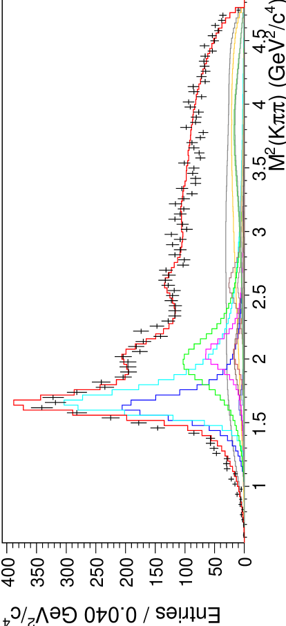
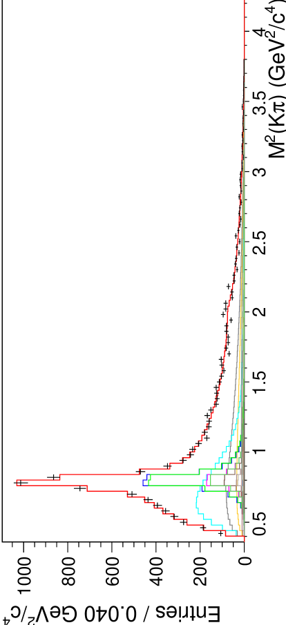
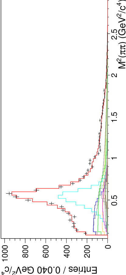
Figure 18: Results of signal-region fits for $B^{+}\rightarrow J/\psi K^{+}\pi^{+}\pi^{-}$. Data (points) and fits (histograms) are shown projected onto the three axes. The fit components are color coded as shown in Fig. 19.

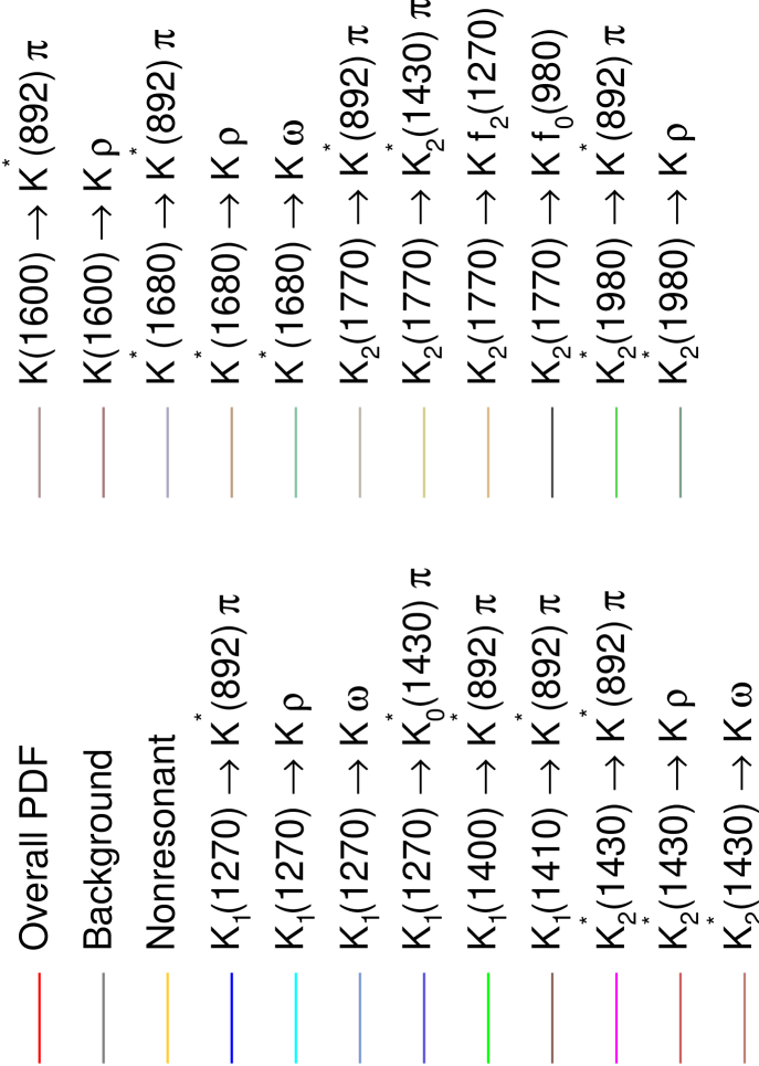
Figure 19: Legend for Figs. 18, 22, 20, 23, 21, and 24.

Similarly, Table 6 shows the fitted parameters for $B^{+}\rightarrow\psi^{\prime}K^{+}\pi^{+}\pi^{-}$ signal-region data, as well as the corresponding decay fractions. Figure 20 shows the fitted PDF and data projected onto the three axes, while Fig. 23 shows $M^{2}(K\pi)$ and $M^{2}(\pi\pi)$ projections for slices in $M^{2}(K\pi\pi)$. In this fit, $\ell=638.3$, while $\chi^{2}=180.1$ with $N_{\mathrm{bins}}=168$ and $N_{\mathrm{par}}=10$.

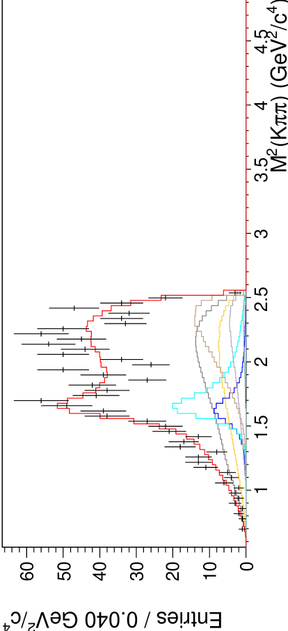
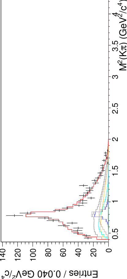
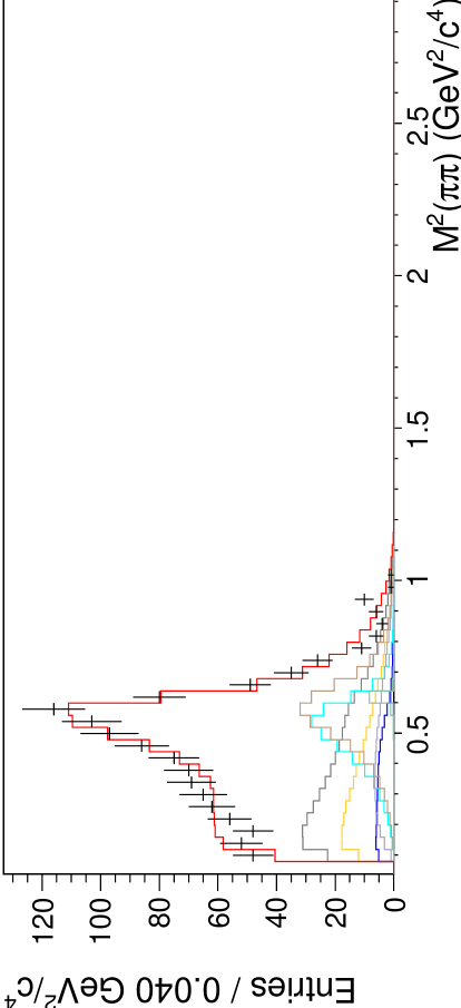
Figure 20: Results of signal-region fits for $B^{+}\rightarrow\psi^{\prime}K^{+}\pi^{+}\pi^{-}$. Data (points) and fits (histograms) are shown projected onto the three axes. The fit components are color coded as shown in Fig. 19.

Finally, the $B^{+}\rightarrow J/\psi K^{+}\pi^{+}\pi^{-}$ signal-region data are fitted again, this time floating the mass and width of the $K_{1}(1270)$. The fitted mass and width are

$$M_{K_{1}(1270)} = (1248.1\pm 3.3\pm 1.4)~{}{\mathrm{MeV}}/c^{2},$$ (38)

$$\Gamma_{K_{1}(1270)} = (119.5\pm 5.2\pm 6.7)~{}{\mathrm{MeV}}/c^{2}.$$ (39)

Table 7 shows the fitted parameters, along with the corresponding decay fractions. Figure 21 shows the fitted PDF and data projected onto the three axes, while Fig. 24 shows $M^{2}(K\pi)$ and $M^{2}(\pi\pi)$ projections for slices in $M^{2}(K\pi\pi)$. In this fit, $\ell=-10525.3$, while $\chi^{2}=1404.4$ with $N_{\mathrm{bins}}=1202$ and $N_{\mathrm{par}}=30$.

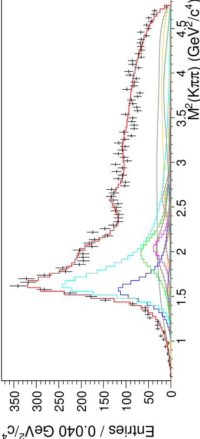
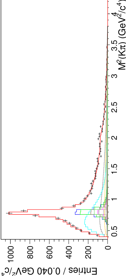
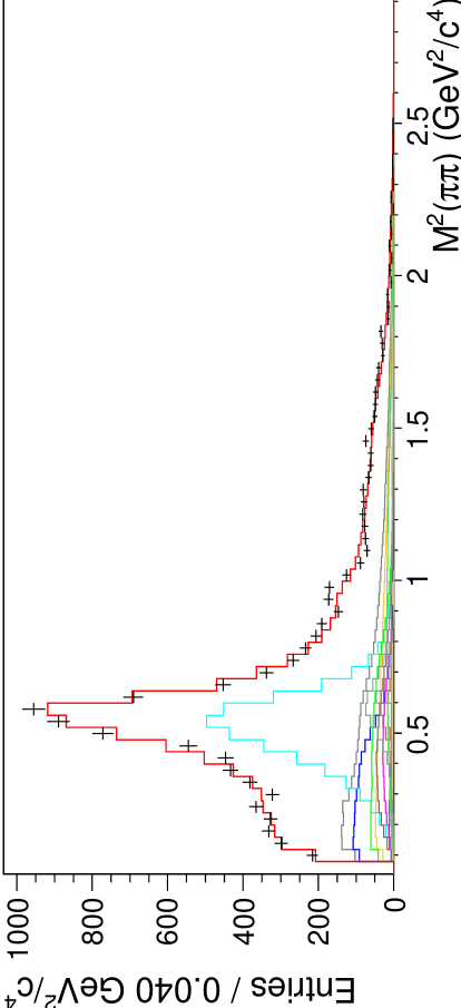
Figure 21: Results of signal-region fits for $B^{+}\rightarrow J/\psi K^{+}\pi^{+}\pi^{-}$, with the mass and width of the $K_{1}(1270)$ floated. Data (points) and fits (histograms) are shown projected onto the three axes. The fit components are color coded as shown in Fig. 19.

A comparison of Tables 5 and 7 reveals that in many cases, the effect of floating the mass and width of the $K_{1}(1270)$ results in a substantial decrease of the systematic error, which is somewhat offset by an increase in the corresponding statistical error. In particular, the $K_{1}(1270)\rightarrow K^{*}(892)\pi$ decay fraction is especially sensitive to the $K_{1}(1270)$ mass and width.

In any fit involving many floating parameters, local likelihood maxima can present a problem. To ensure that the fit results are global maxima, $100$ additional fits were performed for each of the three cases, selecting random starting values for the parameters. None of these fits yielded better likelihoods than those presented above. The local maxima encountered in the course of this test are discussed in the Appendix.

Table 5: Fitted parameters of the signal function for $B^{+}\rightarrow J/\psi K^{+}\pi^{+}\pi^{-}$, along with the corresponding decay fractions.

$J_{1}$	Submode	Modulus			Phase (radians)			Decay fraction
	Nonresonant $K^{+}\pi^{+}\pi^{-}$	$1.0$ (fixed)			$0$ (fixed)			$0.152$ $~{}\pm~{}$	$0.013$ $~{}\pm~{}$	$0.028$
	$K_{1}(1270)\rightarrow K^{*}(892)\pi$	$0.962$ $\,\pm\,$	$0.058$ $\,\pm\,$	$0.176$	$0$ (fixed)			$0.232$ $~{}\pm~{}$	$0.017$ $~{}\pm~{}$	$0.058$
	$K_{1}(1270)\rightarrow K\rho$	$1.813$ $\,\pm\,$	$0.090$ $\,\pm\,$	$0.243$	$-0.764$$\,\pm\,$	$0.069$ $\,\pm\,$	$0.127$	$0.383$ $~{}\pm~{}$	$0.016$ $~{}\pm~{}$	$0.036$
$1^{+}$	$K_{1}(1270)\rightarrow K\omega$	$0.198$ $\,\pm\,$	$0.036$ $\,\pm\,$	$0.041$	$1.09$$\,\pm\,$	$0.18$ $\,\pm\,$	$0.18$	$0.0045$ $~{}\pm~{}$	$0.0017$ $~{}\pm~{}$	$0.0014$
	$K_{1}(1270)\rightarrow K_{0}^{*}(1430)\pi$	$0.95$ $\,\pm\,$	$0.16$ $\,\pm\,$	$0.24$	$2.83$$\,\pm\,$	$0.18$ $\,\pm\,$	$0.18$	$0.0157$ $~{}\pm~{}$	$0.0052$ $~{}\pm~{}$	$0.0049$
	$K_{1}(1400)\rightarrow K^{*}(892)\pi$	$0.894$ $\,\pm\,$	$0.066$ $\,\pm\,$	$0.125$	$-2.300$$\,\pm\,$	$0.044$ $\,\pm\,$	$0.078$	$0.223$ $~{}\pm~{}$	$0.026$ $~{}\pm~{}$	$0.036$
$1^{-}$	$K^{*}(1410)\rightarrow K^{*}(892)\pi$	$0.516$ $\,\pm\,$	$0.090$ $\,\pm\,$	$0.103$	$0$ (fixed)			$0.047$ $~{}\pm~{}$	$0.016$ $~{}\pm~{}$	$0.015$
	$K_{2}^{*}(1430)\rightarrow K^{*}(892)\pi$	$0.663$ $\,\pm\,$	$0.051$ $\,\pm\,$	$0.085$	$0$ (fixed)			$0.088$ $~{}\pm~{}$	$0.011$ $~{}\pm~{}$	$0.011$
	$K_{2}^{*}(1430)\rightarrow K\rho$	$0.371$ (fixed)			$-1.12$$\,\pm\,$	$0.22$ $\,\pm\,$	$0.29$	$0.0233$ (fixed)
$2^{+}$	$K_{2}^{*}(1430)\rightarrow K\omega$	$0.040$ (fixed)			$0.58$$\,\pm\,$	$0.51$ $\,\pm\,$	$0.27$	$0.00036$ (fixed)
	$K_{2}^{*}(1980)\rightarrow K^{*}(892)\pi$	$0.775$ $\,\pm\,$	$0.054$ $\,\pm\,$	$0.118$	$-1.59$$\,\pm\,$	$0.15$ $\,\pm\,$	$0.14$	$0.0739$ $~{}\pm~{}$	$0.0073$ $~{}\pm~{}$	$0.0095$
	$K_{2}^{*}(1980)\rightarrow K\rho$	$0.660$ $\,\pm\,$	$0.048$ $\,\pm\,$	$0.101$	$0.86$$\,\pm\,$	$0.22$ $\,\pm\,$	$0.21$	$0.0613$ $~{}\pm~{}$	$0.0058$ $~{}\pm~{}$	$0.0059$
	$K(1600)\rightarrow K^{*}(892)\pi$	$0.131$ $\,\pm\,$	$0.021$ $\,\pm\,$	$0.024$	$0$ (fixed)			$0.0187$ $~{}\pm~{}$	$0.0058$ $~{}\pm~{}$	$0.0050$
	$K(1600)\rightarrow K\rho$	$0.193$ $\,\pm\,$	$0.017$ $\,\pm\,$	$0.029$	$-0.27$$\,\pm\,$	$0.27$ $\,\pm\,$	$0.18$	$0.0424$ $~{}\pm~{}$	$0.0062$ $~{}\pm~{}$	$0.0110$
	$K_{2}(1770)\rightarrow K^{*}(892)\pi$	$0.122$ $\,\pm\,$	$0.021$ $\,\pm\,$	$0.026$	$2.22$$\,\pm\,$	$0.49$ $\,\pm\,$	$0.37$	$0.0164$ $~{}\pm~{}$	$0.0055$ $~{}\pm~{}$	$0.0061$
$2^{-}$	$K_{2}(1770)\rightarrow K_{2}^{*}(1430)\pi$	$0.286$ $\,\pm\,$	$0.043$ $\,\pm\,$	$0.044$	$1.78$$\,\pm\,$	$0.39$ $\,\pm\,$	$0.24$	$0.0100$ $~{}\pm~{}$	$0.0028$ $~{}\pm~{}$	$0.0020$
	$K_{2}(1770)\rightarrow Kf_{2}(1270)$	$0.444$ $\,\pm\,$	$0.069$ $\,\pm\,$	$0.077$	$2.30$$\,\pm\,$	$0.37$ $\,\pm\,$	$0.32$	$0.0124$ $~{}\pm~{}$	$0.0033$ $~{}\pm~{}$	$0.0022$
	$K_{2}(1770)\rightarrow Kf_{0}(980)$	$0.113$ $\,\pm\,$	$0.029$ $\,\pm\,$	$0.024$	$1.83$$\,\pm\,$	$0.45$ $\,\pm\,$	$0.53$	$0.0034$ $~{}\pm~{}$	$0.0017$ $~{}\pm~{}$	$0.0011$

Table 6: Fitted parameters of the signal function for $B^{+}\rightarrow\psi^{\prime}K^{+}\pi^{+}\pi^{-}$, along with the corresponding decay fractions.

$J_{1}$	Submode	Modulus			Phase (radians)			Decay Fraction
	Nonresonant $K^{+}\pi^{+}\pi^{-}$	$1.0$ (fixed)			$0$ (fixed)			$0.253$ $~{}\pm~{}$	$0.045$ $~{}\pm~{}$	$0.102$
	$K_{1}(1270)\rightarrow K^{*}(892)\pi$	$0.213$ $\,\pm\,$	$0.037$ $\,\pm\,$	$0.049$	$0$ (fixed)			$0.090$ $~{}\pm~{}$	$0.024$ $~{}\pm~{}$	$0.013$
$1^{+}$	$K_{1}(1270)\rightarrow K\rho$	$0.513$ $\,\pm\,$	$0.070$ $\,\pm\,$	$0.141$	$-0.66$$\,\pm\,$	$0.26$ $\,\pm\,$	$0.11$	$0.215$ $~{}\pm~{}$	$0.038$ $~{}\pm~{}$	$0.045$
	$K_{1}(1270)\rightarrow K\omega$	$0.048$ $\,\pm\,$	$0.041$ $\,\pm\,$	$0.022$	$-0.37$$\,\pm\,$	$1.21$ $\,\pm\,$	$0.52$	$0.0017$ $~{}\pm~{}$	$0.0033$ $~{}\pm~{}$	$0.0013$
	$K^{*}(1680)\rightarrow K^{*}(892)\pi$	$0.67$ $\,\pm\,$	$0.12$ $\,\pm\,$	$0.15$	$0$ (fixed)			$0.106$ $~{}\pm~{}$	$0.031$ $~{}\pm~{}$	$0.017$
$1^{-}$	$K^{*}(1680)\rightarrow K\rho$	$1.17$ $\,\pm\,$	$0.16$ $\,\pm\,$	$0.32$	$1.27$$\,\pm\,$	$0.24$ $\,\pm\,$	$0.15$	$0.241$ $~{}\pm~{}$	$0.047$ $~{}\pm~{}$	$0.050$
	$K^{*}(1680)\rightarrow K\omega$	$0.233$ $\,\pm\,$	$0.097$ $\,\pm\,$	$0.047$	$-3.06$$\,\pm\,$	$0.43$ $\,\pm\,$	$0.45$	$0.0119$ $~{}\pm~{}$	$0.0106$ $~{}\pm~{}$	$0.0061$

Table 7: Fitted parameters of the signal function for $B^{+}\rightarrow J/\psi K^{+}\pi^{+}\pi^{-}$ when the $K_{1}(1270)$ mass and width are floated, along with the corresponding decay fractions.

$J_{1}$	Submode	Modulus			Phase (radians)			Decay Fraction
	Nonresonant $K^{+}\pi^{+}\pi^{-}$	$1.0$ (fixed)			$0$ (fixed)			$0.142$ $~{}\pm~{}$	$0.013$ $~{}\pm~{}$	$0.026$
	$K_{1}(1270)\rightarrow K^{*}(892)\pi$	$0.882$ $\,\pm\,$	$0.076$ $\,\pm\,$	$0.090$	$0$ (fixed)			$0.168$ $~{}\pm~{}$	$0.023$ $~{}\pm~{}$	$0.012$
	$K_{1}(1270)\rightarrow K\rho$	$2.14$ $\,\pm\,$	$0.12$ $\,\pm\,$	$0.27$	$-0.588$$\,\pm\,$	$0.084$ $\,\pm\,$	$0.110$	$0.430$ $~{}\pm~{}$	$0.018$ $~{}\pm~{}$	$0.027$
$1^{+}$	$K_{1}(1270)\rightarrow K\omega$	$0.289$ $\,\pm\,$	$0.043$ $\,\pm\,$	$0.040$	$1.25$$\,\pm\,$	$0.16$ $\,\pm\,$	$0.14$	$0.00758$ $~{}\pm~{}$	$0.00216$ $~{}\pm~{}$	$0.00076$
	$K_{1}(1270)\rightarrow K_{0}^{*}(1430)\pi$	$1.09$ $\,\pm\,$	$0.18$ $\,\pm\,$	$0.24$	$2.93$$\,\pm\,$	$0.18$ $\,\pm\,$	$0.16$	$0.0184$ $~{}\pm~{}$	$0.0055$ $~{}\pm~{}$	$0.0046$
	$K_{1}(1400)\rightarrow K^{*}(892)\pi$	$0.746$ $\,\pm\,$	$0.085$ $\,\pm\,$	$0.089$	$-2.585$$\,\pm\,$	$0.100$ $\,\pm\,$	$0.076$	$0.145$ $~{}\pm~{}$	$0.029$ $~{}\pm~{}$	$0.017$
$1^{-}$	$K^{*}(1410)\rightarrow K^{*}(892)\pi$	$0.736$ $\,\pm\,$	$0.084$ $\,\pm\,$	$0.098$	$0$ (fixed)			$0.089$ $~{}\pm~{}$	$0.019$ $~{}\pm~{}$	$0.010$
	$K_{2}^{*}(1430)\rightarrow K^{*}(892)\pi$	$0.529$ $\,\pm\,$	$0.064$ $\,\pm\,$	$0.070$	$0$ (fixed)			$0.0525$ $~{}\pm~{}$	$0.0120$ $~{}\pm~{}$	$0.0070$
	$K_{2}^{*}(1430)\rightarrow K\rho$	$0.296$ (fixed)			$-0.61$$\,\pm\,$	$0.39$ $\,\pm\,$	$1.07$	$0.014$ (fixed)
$2^{+}$	$K_{2}^{*}(1430)\rightarrow K\omega$	$0.032$ (fixed)			$1.41$$\,\pm\,$	$0.80$ $\,\pm\,$	$0.25$	$0.00021$ (fixed)
	$K_{2}^{*}(1980)\rightarrow K^{*}(892)\pi$	$0.756$ $\,\pm\,$	$0.060$ $\,\pm\,$	$0.119$	$-1.46$$\,\pm\,$	$0.23$ $\,\pm\,$	$0.22$	$0.0659$ $~{}\pm~{}$	$0.0073$ $~{}\pm~{}$	$0.0088$
	$K_{2}^{*}(1980)\rightarrow K\rho$	$0.685$ $\,\pm\,$	$0.052$ $\,\pm\,$	$0.106$	$1.15$$\,\pm\,$	$0.30$ $\,\pm\,$	$0.20$	$0.0617$ $~{}\pm~{}$	$0.0061$ $~{}\pm~{}$	$0.0065$
	$K(1600)\rightarrow K^{*}(892)\pi$	$0.147$ $\,\pm\,$	$0.021$ $\,\pm\,$	$0.026$	$0$ (fixed)			$0.0222$ $~{}\pm~{}$	$0.0058$ $~{}\pm~{}$	$0.0054$
	$K(1600)\rightarrow K\rho$	$0.171$ $\,\pm\,$	$0.020$ $\,\pm\,$	$0.023$	$-0.21$$\,\pm\,$	$0.29$ $\,\pm\,$	$0.12$	$0.0312$ $~{}\pm~{}$	$0.0065$ $~{}\pm~{}$	$0.0040$
	$K_{2}(1770)\rightarrow K^{*}(892)\pi$	$0.116$ $\,\pm\,$	$0.020$ $\,\pm\,$	$0.029$	$1.93$$\,\pm\,$	$0.52$ $\,\pm\,$	$0.43$	$0.0137$ $~{}\pm~{}$	$0.0049$ $~{}\pm~{}$	$0.0058$
$2^{-}$	$K_{2}(1770)\rightarrow K_{2}^{*}(1430)\pi$	$0.288$ $\,\pm\,$	$0.045$ $\,\pm\,$	$0.045$	$1.81$$\,\pm\,$	$0.40$ $\,\pm\,$	$0.24$	$0.0095$ $~{}\pm~{}$	$0.0027$ $~{}\pm~{}$	$0.0018$
	$K_{2}(1770)\rightarrow Kf_{2}(1270)$	$0.466$ $\,\pm\,$	$0.073$ $\,\pm\,$	$0.080$	$2.22$$\,\pm\,$	$0.36$ $\,\pm\,$	$0.33$	$0.0128$ $~{}\pm~{}$	$0.0035$ $~{}\pm~{}$	$0.0021$
	$K_{2}(1770)\rightarrow Kf_{0}(980)$	$0.118$ $\,\pm\,$	$0.030$ $\,\pm\,$	$0.025$	$1.89$$\,\pm\,$	$0.45$ $\,\pm\,$	$0.53$	$0.0035$ $~{}\pm~{}$	$0.0017$ $~{}\pm~{}$	$0.0011$

    

    

    

    

    

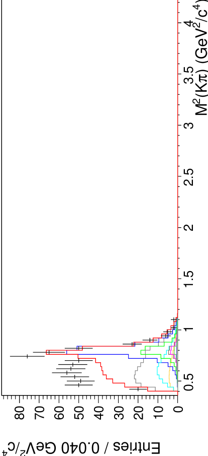
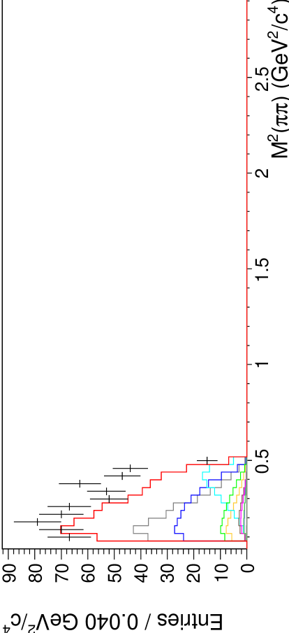
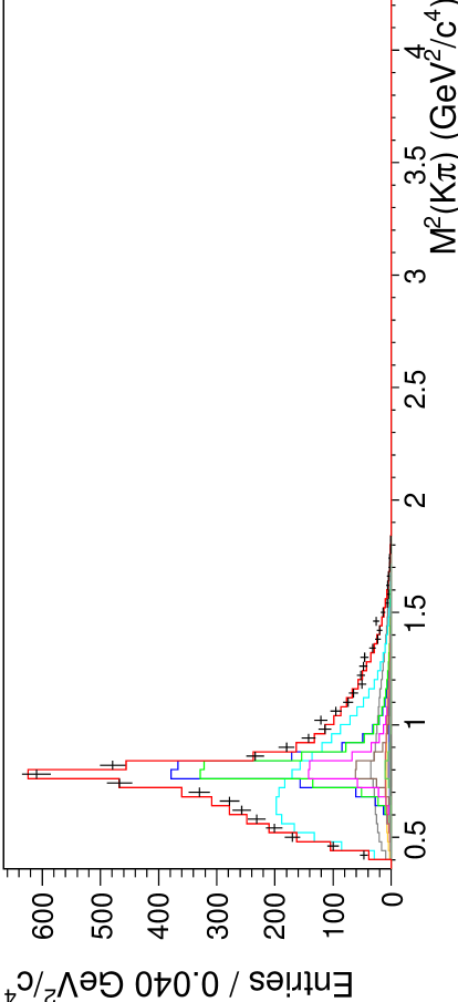
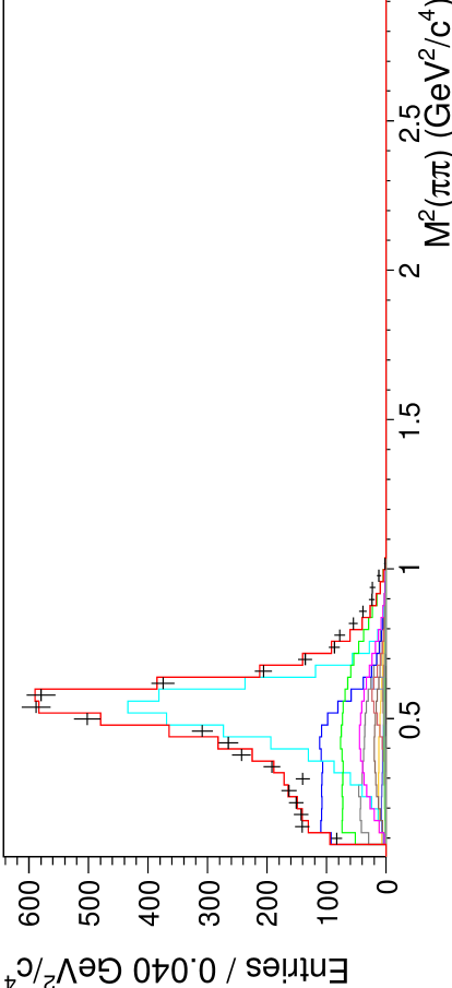
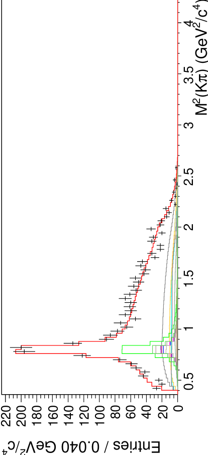
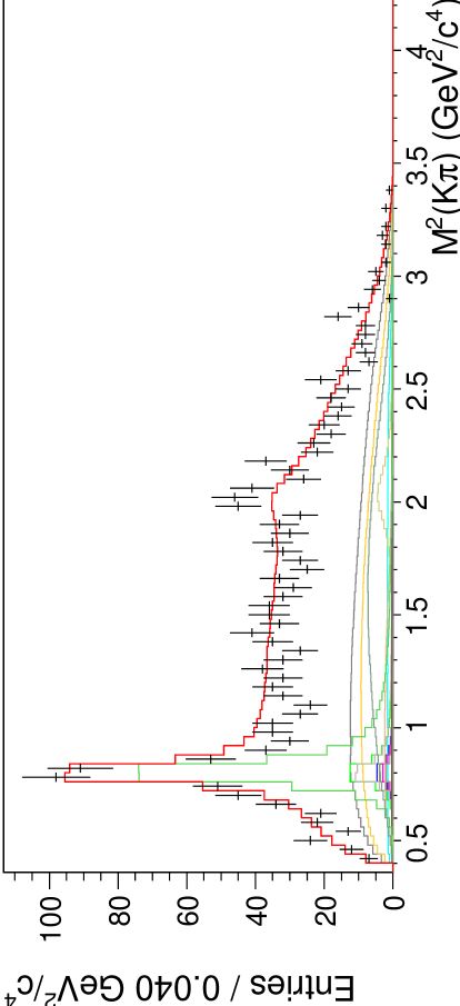
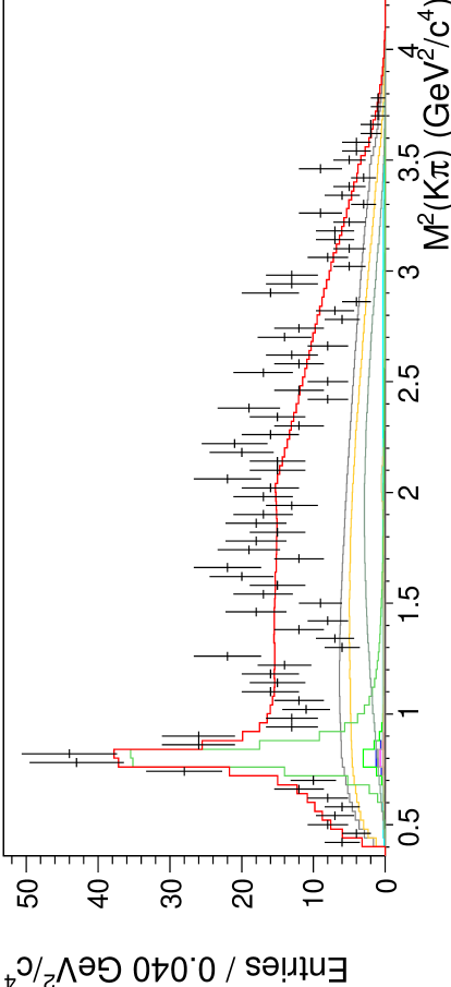
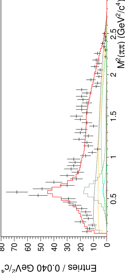
Figure 22: $B^{+}\rightarrow J/\psi K^{+}\pi^{+}\pi^{-}$ signal data (points) and fit results (histograms) for slices in $M^{2}(K\pi\pi)$. The fit components are color coded as shown in Fig. 19.

    

    

    

    

    

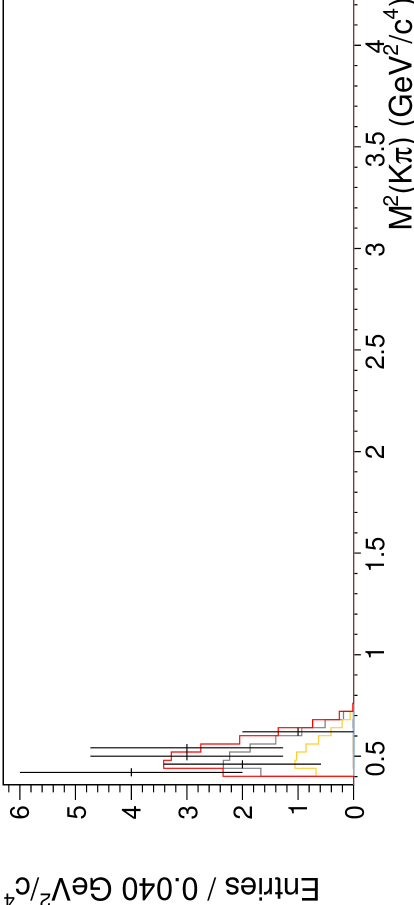
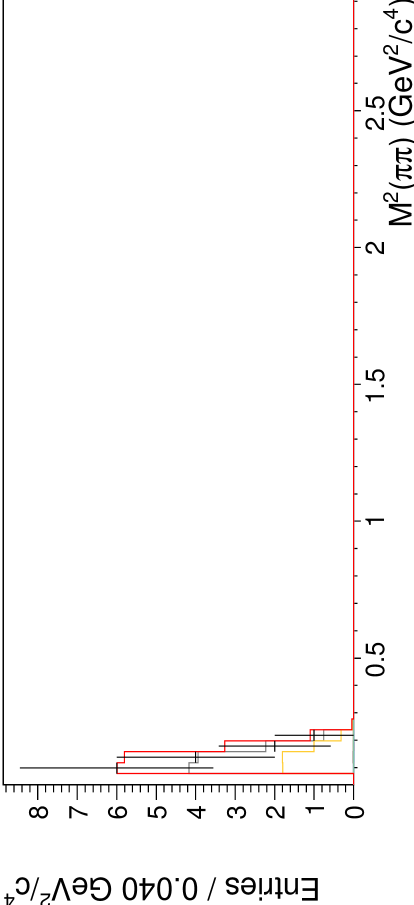
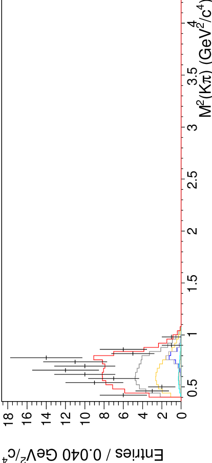
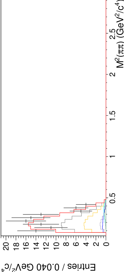
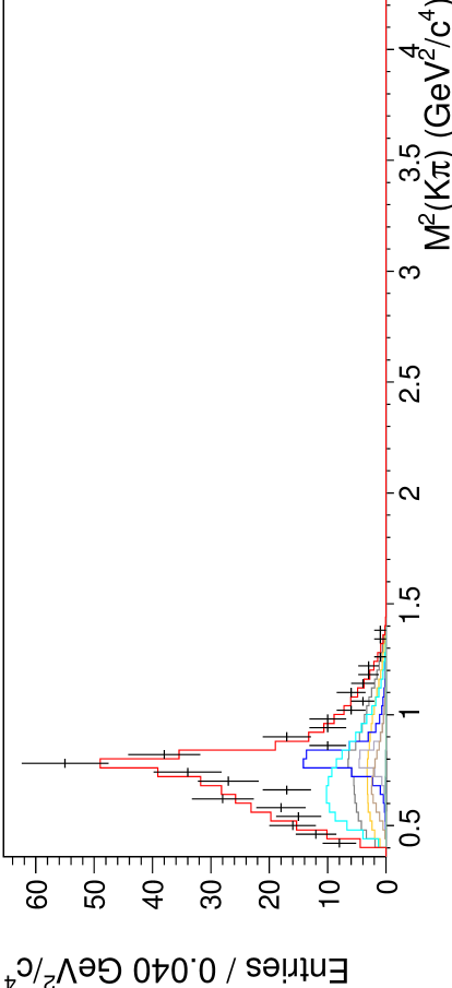
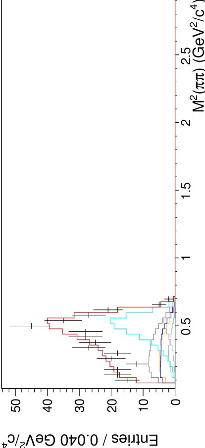
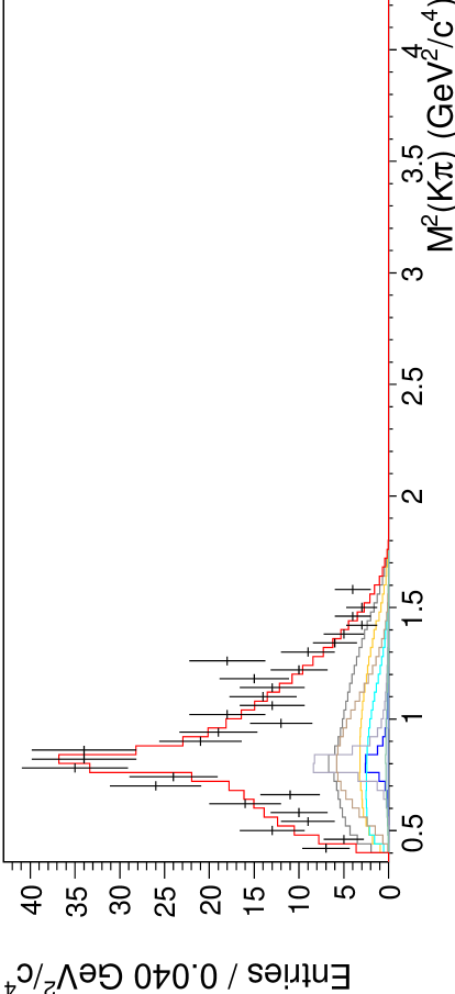
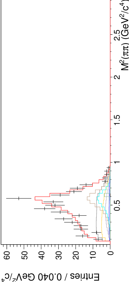
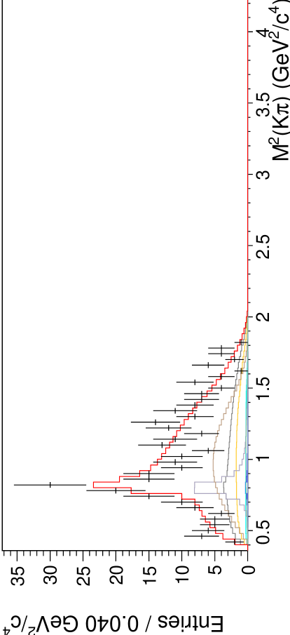
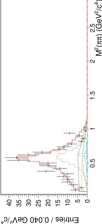
Figure 23: $B^{+}\rightarrow\psi^{\prime}K^{+}\pi^{+}\pi^{-}$ signal data (points) and fit results (histograms) for slices in $M^{2}(K\pi\pi)$. The fit components are color coded as shown in Fig. 19.

    

    

    

    

    

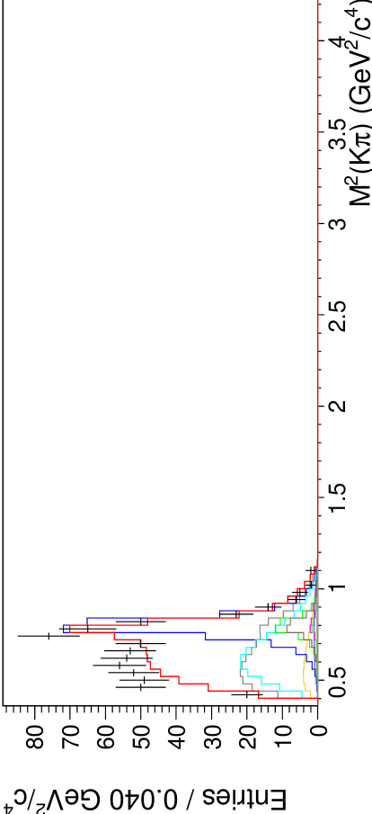
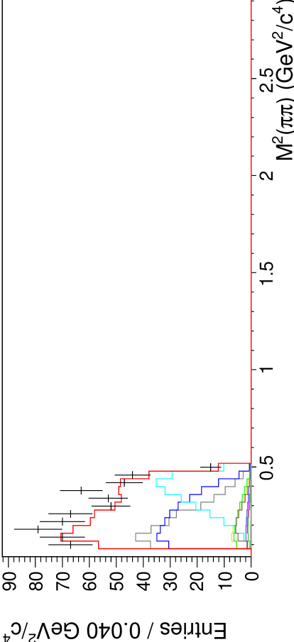
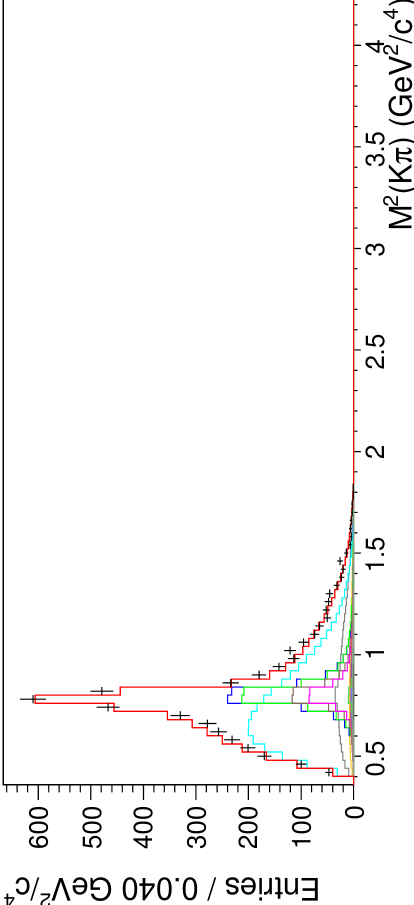
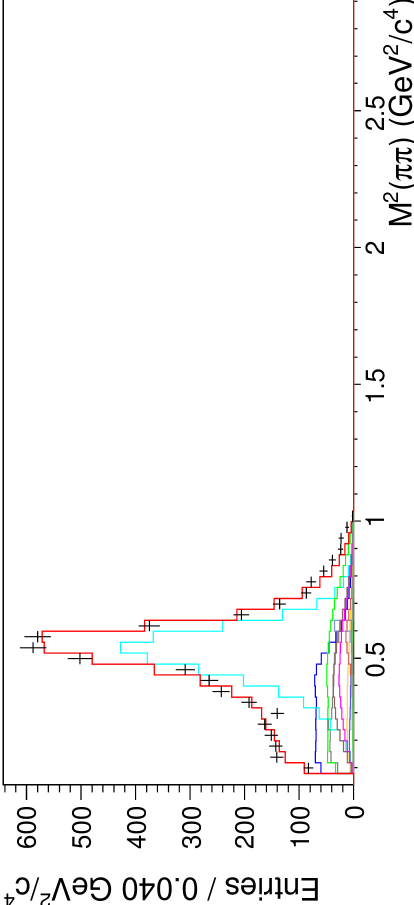
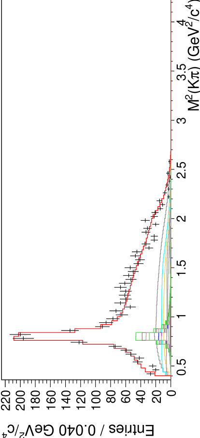
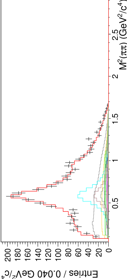
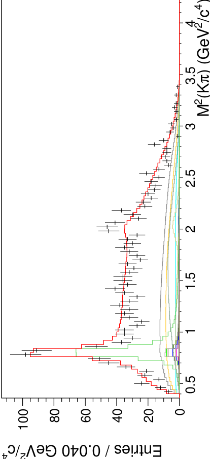
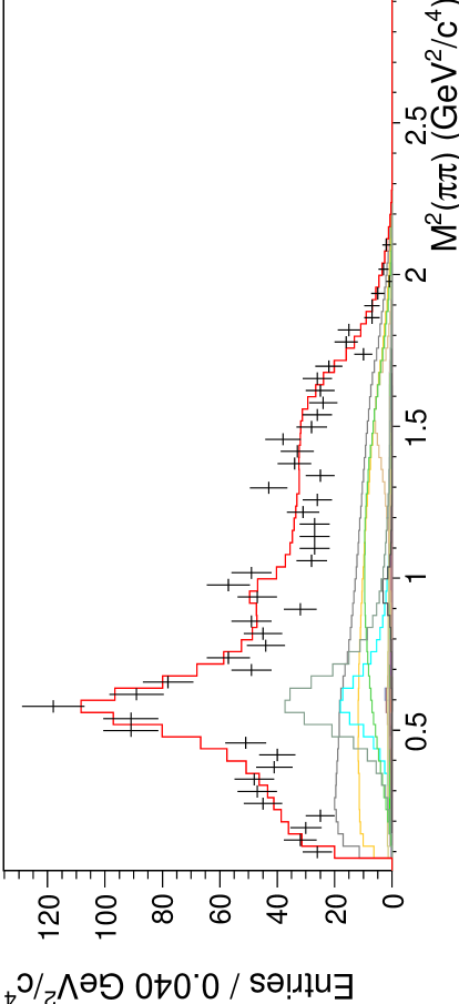
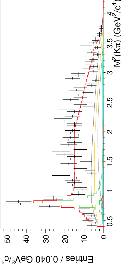
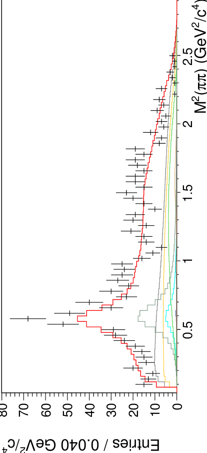
Figure 24: $B^{+}\rightarrow J/\psi K^{+}\pi^{+}\pi^{-}$ signal data (points) and fit results (histograms) for slices in $M^{2}(K\pi\pi)$. The fit components are color coded as shown in Fig. 19. The mass and width of the $K_{1}(1270)$ floated in the fit.

VI.10 Discussion

VI.10.1 Signal components

In choosing the signal components to be included in the fits, the data were used as a guide. As the $K_{1}(1270)$ signal is prominent in both $B^{+}\rightarrow J/\psi K^{+}\pi^{+}\pi^{-}$ and $B^{+}\rightarrow\psi^{\prime}K^{+}\pi^{+}\pi^{-}$ data, the initial fits were done with only $K_{1}(1270)\rightarrow K^{*}(892)\pi$ and $K_{1}(1270)\rightarrow K\rho$ on top of the nonresonant component. Additional decay channels were added successively until a reasonable level of agreement between fit and data was obtained.

As a further guide, the decays $B^{0}\rightarrow J/\psi K^{+}\pi^{-}$ and $B^{0}\rightarrow\psi^{\prime}K^{+}\pi^{-}$ were reconstructed. The observed $K\pi$ mass spectra are shown in Fig. 25. Consistent with the $1^{+}$ spin-parity assignment of the $K_{1}(1270)$, no $K_{1}(1270)\rightarrow K\pi$ signal appears in these spectra. In both modes, a small peak can be seen near $1.4~{}{\mathrm{GeV}}/c^{2}$ in $M(K\pi)$; this may have contributions from $K^{*}(1410)$ or $K_{2}^{*}(1430)$, as well as $K_{0}^{*}(1430)$. The absence of a $K^{*}(1680)$ peak in $B^{0}\rightarrow J/\psi K^{+}\pi^{-}$ is noteworthy, although a precise statement would require an analysis of the efficiency and phase space for these modes. In $B^{0}\rightarrow\psi^{\prime}K^{+}\pi^{-}$, the kinematically-allowed $M(K\pi)$ region does not allow any conclusions to be drawn about the presence or absence of a low $K^{*}(1680)$ tail.

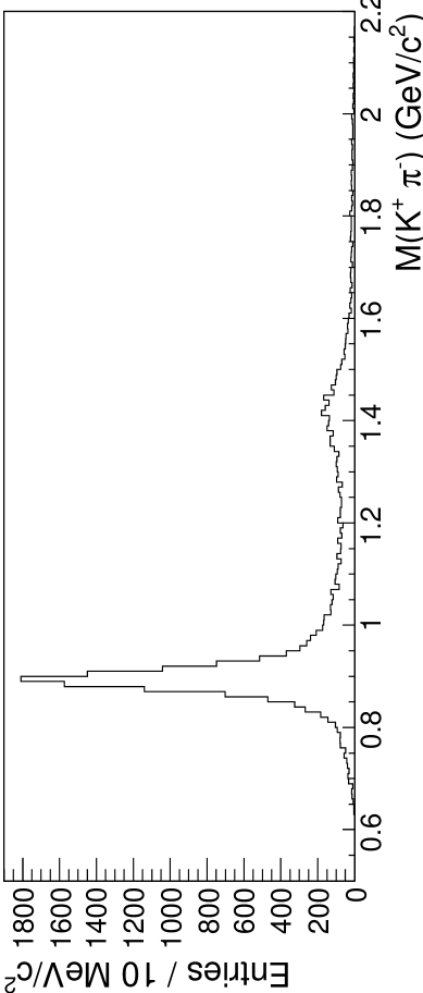
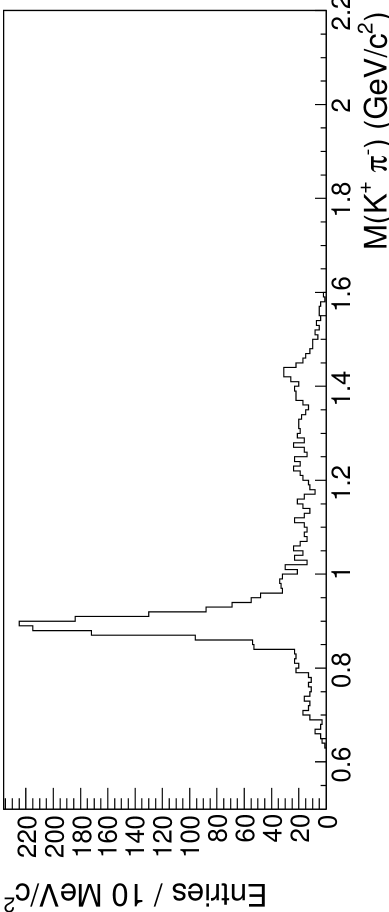
Figure 25: Observed $K\pi$ mass spectra for $B^{0}\rightarrow J/\psi K^{+}\pi^{-}$ (top) and $B^{0}\rightarrow\psi^{\prime}K^{+}\pi^{-}$ (bottom) data.

VI.10.2 Interference effects

The inclusion of interference among submodes sharing the same initial-state spin-parity is essential to obtaining good fits to the data. In particular, dramatic interference effects are observed between $K_{1}(1270)\rightarrow K^{*}(892)\pi$ and $K_{1}(1270)\rightarrow K\rho$, as well as between $K_{1}(1270)\rightarrow K\rho$ and $K_{1}(1270)\rightarrow K\omega$.

Figure 27 shows scatterplots of signal-region $B^{+}\rightarrow J/\psi K^{+}\pi^{+}\pi^{-}$ data over the three coordinates. Interference between $K_{1}(1270)\rightarrow K^{*}(892)\pi$ and $K_{1}(1270)\rightarrow K\rho$ is responsible for the weakening of the latter signal at $M(K\pi)>M_{K^{*}(892)}$. Although the four-body phase space decreases with increasing $M(K\pi)$, this is not sufficient to account for the abrupt falloff. To describe the data in this region, the two modes must be added coherently.

Since the previously-measured pdg08 branching fraction for $K_{1}(1270)\rightarrow K\omega$ is small compared to that for $K_{1}(1270)\rightarrow K\rho$, and since only $1.5\%$ of $\omega$’s decay to $\pi^{+}\pi^{-}$, one might expect $K_{1}(1270)\rightarrow K\omega$ to play a negligible role in this analysis. Nonetheless, since the $\omega$ is much narrower than the $\rho$, it significantly distorts the observed $\rho$ line shape through interference lafferty:1993 . In Fig. 26, the $M^{2}(\pi\pi)$ projections of Figs. 18, 20 and 21 are finely binned to demonstrate this interference pattern, which is accurately modeled by the PDFs.

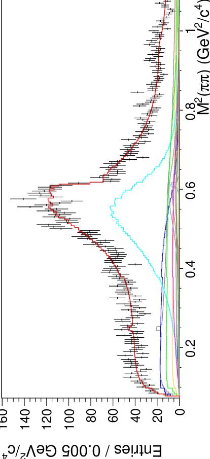
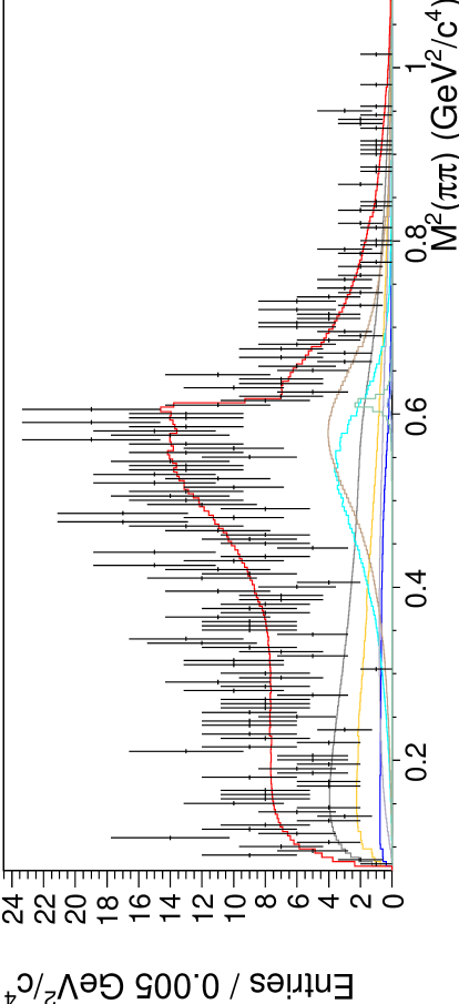
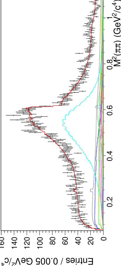
Figure 26: Finely-binned projections onto the $M^{2}(\pi\pi)$ axis of signal-region data (fits) and fit results (histograms) for $B^{+}\rightarrow J/\psi K^{+}\pi^{+}\pi^{-}$ (top), $B^{+}\rightarrow\psi^{\prime}K^{+}\pi^{+}\pi^{-}$ (middle), and $B^{+}\rightarrow J/\psi K^{+}\pi^{+}\pi^{-}$ with the mass and width of the $K_{1}(1270)$ floated (bottom). The fit components are color coded as shown in Fig. 13. The discontinuity at the $\omega$ mass is due to $\rho$-$\omega$ interference.

The peculiar shape of the observed $\rho$-$\omega$ interference pattern is caused by kinematic effects. The largest contribution to the $\rho$ signal comes from $K_{1}(1270)\rightarrow K\rho$, which straddles the edge of phase space, as can be seen in the middle panel of Fig. 27. The distortion that is caused by this kinematic cutoff is taken into account automatically by integrating the signal function only over the kinematically-allowed region, as described in Sec. VI.1. Modeling the data accurately requires including $\rho$-$\omega$ interference, incorporating the four-body phase space factor into the signal function, and integrating the signal function over only the kinematically-allowed phase space.

   

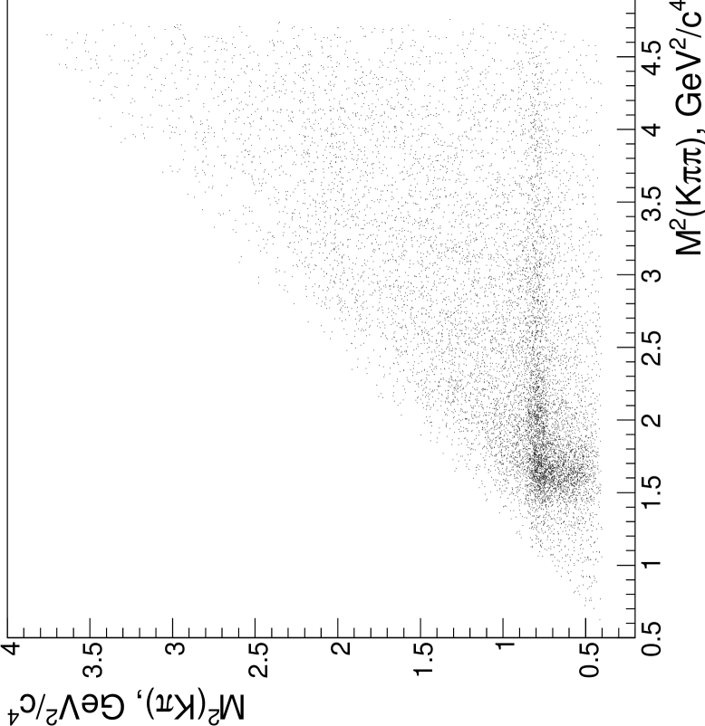
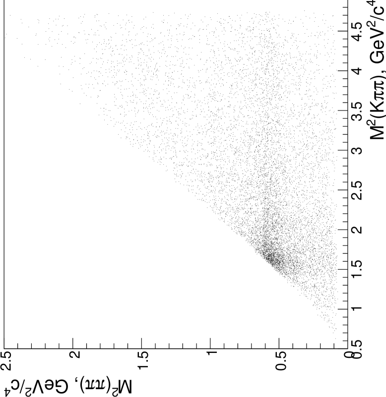
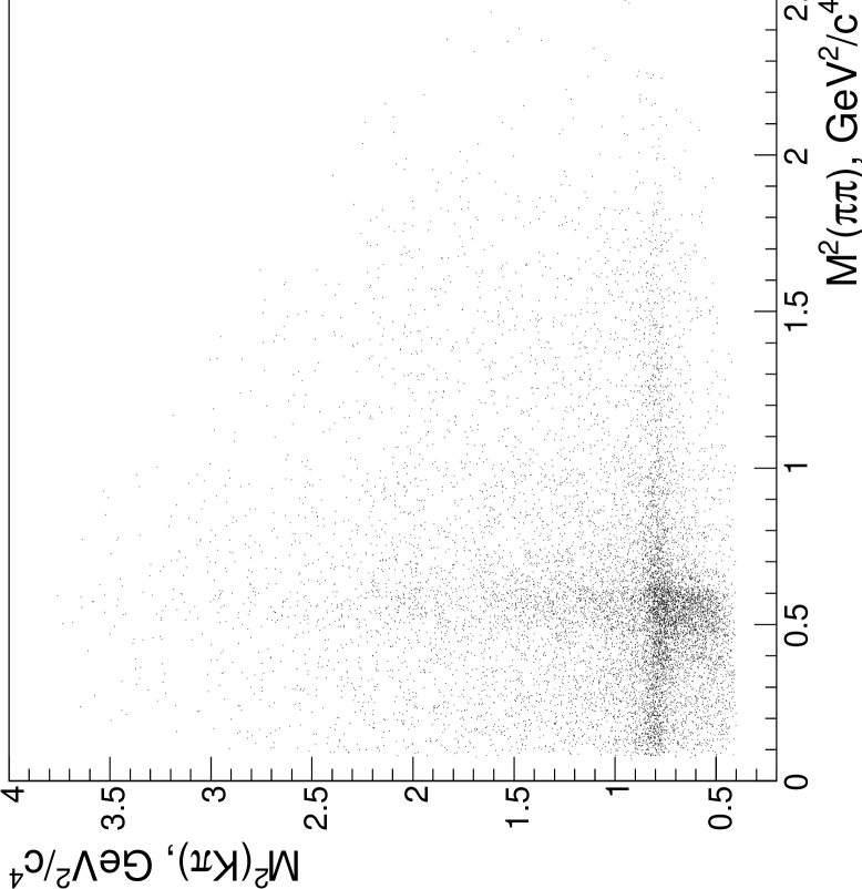
Figure 27: Scatterplots for $B^{+}\rightarrow J/\psi K^{+}\pi^{+}\pi^{-}$ data, showing $M^{2}(K\pi)$ versus $M^{2}(K\pi\pi)$ (left), $M^{2}(\pi\pi)$ versus $M^{2}(K\pi\pi)$ (middle), and $M^{2}(K\pi)$ versus $M^{2}(\pi\pi)$ (right). Interference between the $K\rho$ and $K^{*}(892)\pi$ submodes of the $K_{1}(1270)$ is responsible for the abrupt fading of the $K^{*}(892)$ signal at $M(K\pi)>M_{K^{*}(892)}$. The effect is most apparent in the left and right plots. Scatterplots for $B^{+}\rightarrow\psi^{\prime}K^{+}\pi^{+}\pi^{-}$ data are similar but limited by statistics.

VI.10.3 The $L$ region

The $M(K\pi\pi)$ region between $1.5$ and $2.0~{}{\mathrm{GeV}}/c^{2}$, historically referred to as the $L$ region, comprises several wide, overlapping resonances amaldi:1976 ; otter:1979 ; daum:1981 . The large uncertainties in the masses and widths of the known states in this region make it difficult to characterize this region in this analysis. The model presented here is not necessarily the only one supported by the data.

To describe the structure observed at $2.6~{}{\mathrm{GeV}}^{2}/c^{4}$ in the $M^{2}(K\pi\pi)$ distribution of $B^{+}\rightarrow J/\psi K^{+}\pi^{+}\pi^{-}$, a peak with a mass of $1.605~{}{\mathrm{GeV}}/c^{2}$ and a width of $115~{}{\mathrm{MeV}}/c^{2}$ is included in the fit, decaying to $K^{*}(892)\pi$ and $K\rho$. This peak, which is referred to as $K(1600)$ in this paper, may be the $K_{2}(1580)$, an as-yet unconfirmed $J^{P}=2^{-}$ state that has previously been observed decaying to $K^{*}(892)\pi$ otter:1979 .

As can be seen in Fig. 22, the high end of the $M^{2}(K\pi\pi)$ spectrum of $B^{+}\rightarrow J/\psi K^{+}\pi^{+}\pi^{-}$ exhibits $K^{*}$ and $\rho$ signals. To fit the data in this region, we include a $K_{2}^{*}(1980)$ resonance, which is another state that currently requires confirmation.

Even after including $K(1600)$ and $K_{2}^{*}(1980)$ resonances in the $B^{+}\rightarrow J/\psi K^{+}\pi^{+}\pi^{-}$ fit, a slight enhancement remains around $3~{}{\mathrm{GeV}}^{2}/c^{4}$ in $M^{2}(K\pi\pi)$. A $K_{2}(1770)$ signal is therefore also included, with its known decays to $K^{*}(892)\pi$, $K_{2}^{*}(1430)\pi$, $Kf_{0}(980)$, and $Kf_{2}(1270)$.

Fitting the $B^{+}\rightarrow\psi^{\prime}K^{+}\pi^{+}\pi^{-}$ data is more difficult still, as there are fewer events to analyze, and only a small portion of the $L$-region is within the kinematic limits of the decay. In addition to the $K_{1}(1270)$ signal, the $M^{2}(K\pi\pi)$ spectrum contains what appears to be the low-mass tail of at least one high-mass resonance. As Fig. 23 shows, there are clear $K^{*}(892)$ and $\rho$ peaks at high $M^{2}(K\pi\pi)$; these are not reproduced by the PDF if no high-mass resonance is included in the model. If the enhancement is modeled as a single resonance, the data favor a mass of roughly $1.7~{}{\mathrm{GeV}}/c^{2}$ and a width of $400$-$500~{}{\mathrm{MeV}}/c^{2}$. In this analysis, the enhancement is modeled as the $K^{*}(1680)$. The data do not preclude other possibilities, such as the $K_{2}(1770)$. Indeed, the hint of $f_{0}(980)$ in the last $M^{2}(K\pi\pi)$ slice in Fig. 23 cannot come from a $1^{-}$ state such as the $K^{*}(1680)$, or from a $2^{+}$ state such as the $K_{2}^{*}(1430)$.

VI.10.4 Comparison with previous measurements

It is interesting to compare the relative decay fractions for $K_{1}(1270)$ submodes in the $B^{+}\rightarrow J/\psi K^{+}\pi^{+}\pi^{-}$ fits to previous measurements of $K_{1}(1270)$ branching fractions. For this purpose, we use the decay fractions with phase space shown in Tables 5 and 7, include isospin factors, and assume branching fractions of $(1.53^{+0.11}_{-0.13})\%$ for $\omega\rightarrow\pi^{+}\pi^{-}$, and $(93\pm 10)\%$ for $K_{0}^{*}(1430)\rightarrow K\pi$ pdg08 . The calculation neglects the systematic errors in the decay fractions and assumes that the statistical errors among the decay fractions are uncorrelated. Moreover, it assumes that the $K_{1}(1270)$ decays only to $K^{*}(892)\pi$, $K\rho$, $K\omega$, and $K_{0}^{*}(1430)\pi$, and neglects interference among these decay channels. The comparison is shown in Table 8. While the ratios of the $K_{1}(1270)$ branching fractions to $K^{*}(892)\pi$, $K\rho$, and $K\omega$ are consistent with the previously-measured values, the branching fraction to $K_{0}^{*}(1430)\pi$ is significantly smaller.

Table 8: Comparison of branching fractions for $K_{1}(1270)$ decays according to the Particle Data Group (PDG) pdg08 and based on the results shown in Table 5 (fit 1) and Table 7 (fit 2). See text for assumptions.

$K_{1}(1270)$	Branching Fraction (%)
Decay mode	PDG		Fit 1		Fit 2
$K\rho$	$42$$~{}\pm~{}$	$6$	$57.3$$~{}\pm~{}$	$3.5$	$58.4$$~{}\pm~{}$	$4.3$
$K_{0}^{*}(1430)\pi$	$28$$~{}\pm~{}$	$4$	$1.90$$~{}\pm~{}$	$0.66$	$2.01$$~{}\pm~{}$	$0.64$
$K^{*}(892)\pi$	$16$$~{}\pm~{}$	$5$	$26.0$$~{}\pm~{}$	$2.1$	$17.1$$~{}\pm~{}$	$2.3$
$K\omega$	$11$$~{}\pm~{}$	$2$	$14.8$$~{}\pm~{}$	$4.7$	$22.5$$~{}\pm~{}$	$5.2$
$Kf_{0}(1370)$	$3$$~{}\pm~{}$	$2$	N/A		N/A

VI.10.5 Mass and width of the $K_{1}(1270)$

As shown in Sec. VI.9, the data favor a smaller mass and a larger width for the $K_{1}(1270)$ than the Particle Data Group (PDG) values. This is mainly due to the excess of $K^{*}(892)$ and $\rho$ at low $M^{2}(K\pi\pi)$, as can be ascertained by comparing the first row of plots in Figs. 22 and 24. The measured mass and width agree remarkably well with Ref. astier:1969, and are also consistent with Ref. asner:2000, .

VI.10.6 Limitations of the method

There are large uncertainties in the masses and widths of many of the states included in the fits, as can be seen in Table 4. Although this is taken into account in calculating the systematic error, it nonetheless limits the accuracy of the model.

In $B^{+}\rightarrow\psi^{\prime}K^{+}\pi^{+}\pi^{-}$, the small sample size and the kinematic cutoff limit the conclusions that can be drawn about the signal components. In $B^{+}\rightarrow J/\psi K^{+}\pi^{+}\pi^{-}$, the sample size is larger, but a further limitation is imposed by the increase in computation time as more parameters are added to the fit. Each additional decay channel that is included in the signal function contributes a modulus and possibly a phase to be varied in the fit. Since the normalization integral of the signal function in Eq. 16 depends on the values of the parameters $\vec{a}$, the integration must be performed for each set of parameters attempted by the fitter. While the step size used in the numerical integration can be increased to speed up the process, it must be small enough to allow the PDF to resolve the structures in the data. In particular, the $\rho$-$\omega$ interference pattern can be fitted with a step size of $0.01~{}{\mathrm{GeV}}^{2}/c^{4}$, but not with a step size of $0.02~{}{\mathrm{GeV}}^{2}/c^{4}$. As a consequence of the finite processor speed, not every possible decay channel can be included in the fit. The model is necessarily incomplete.

The large nonresonant component seen in both $B^{+}\rightarrow J/\psi K^{+}\pi^{+}\pi^{-}$ and $B^{+}\rightarrow\psi^{\prime}K^{+}\pi^{+}\pi^{-}$ may be an indication of contributions from additional wide kaon excitations. It may also incorporate some misreconstructed resonant signal. While the nonresonant component is assumed in this analysis to be distributed according to phase space, this assumption may be inaccurate. There are currently no accepted models of nonresonant $B$-meson decays.

It is difficult, in an analysis like the one presented here, to determine the significance of a given component of the signal. An improvement in the likelihood upon the addition of a new resonance to the signal function indicates only that the model is incomplete, not necessarily that the data contain the particular resonance. Furthermore, unless the model is accurate in every other way, floating the mass and width of a particle in the fit may not yield a reliable result, as the fitter may set these parameters to compensate for the model’s deficiencies. This is especially important in the high-$M^{2}(K\pi\pi)$ region, where the statistics are limited and there are large uncertainties in the masses and widths of the resonances included in the signal function. Thus, although the $K(1600)$ component of the signal function for $B^{+}\rightarrow J/\psi K^{+}\pi^{+}\pi^{-}$ greatly improves the quality of the fit, it is difficult to claim that it is a single particle, let alone measure its mass and width.

VII Conclusions

Using data recorded by the Belle detector, we have measured branching fractions for the decays $B^{+}\rightarrow J/\psi K^{+}\pi^{+}\pi^{-}$ and $B^{+}\rightarrow\psi^{\prime}K^{+}\pi^{+}\pi^{-}$ with improved precision (see Sec. V.2). We have also performed amplitude analyses in three dimensions—$M^{2}(K\pi\pi)$, $M^{2}(K\pi)$, and $M^{2}(\pi\pi)$—to determine the resonant structure of the $K^{+}\pi^{+}\pi^{-}$ final state in these decays (see Sec. VI.9).

We have shown that the $K_{1}(1270)$, which is the dominant component of the $K^{+}\pi^{+}\pi^{-}$ final state in $B^{+}\rightarrow J/\psi K^{+}\pi^{+}\pi^{-}$, is also prominent in $B^{+}\rightarrow\psi^{\prime}K^{+}\pi^{+}\pi^{-}$. The large sample available for the former decay reveals a small peak at $M(K\pi\pi)\approx 1.4~{}{\mathrm{GeV}}/c^{2}$. Our three-dimensional fits represent a first attempt to determine the components of this peak.

Performing an unbinned fit in three dimensions exploits practically all of the information available in the data. While it is relatively easy to obtain a good fit in one dimension, requiring a fit that succeeds in three dimensions greatly restricts the class of successful models. With high statistics, it is possible to use interference effects and the spin-dependent angular distribution of the final state to distinguish overlapping resonances. In particular, we have shown that $\rho$-$\omega$ interference cannot be neglected in studying $K_{1}(1270)$ decays to $K\pi^{+}\pi^{-}$ final states.

The large size of the $B^{+}\rightarrow J/\psi K^{+}\pi^{+}\pi^{-}$ data sample allows us to measure the mass and width of the $K_{1}(1270)$ with improved precision (see Eqs. 38 and 39). These values differ considerably from previously-published values pdg08 . The analysis of these data also provides information on the relative strengths of $K_{1}(1270)$ decays to $K\rho$, $K\omega$, $K^{*}(892)\pi$, and $K_{0}^{*}(1430)\pi$ final states (see Table 8). While the results are consistent with previous measurements for the first three modes, they indicate a much smaller rate of decay to $K_{0}^{*}(1430)\pi$ than previously accepted.

Although more data are required to clarify the structure of the high $M^{2}(K^{+}\pi^{+}\pi^{-})$ region in both $B^{+}\rightarrow J/\psi K^{+}\pi^{+}\pi^{-}$ and $B^{+}\rightarrow\psi^{\prime}K^{+}\pi^{+}\pi^{-}$, we have shown that this region contains broad resonances that decay to $K^{*}(892)\pi$ and $K\rho$ final states.

The analysis presented in this paper demonstrates that the decay modes $B^{+}\rightarrow J/\psi K^{+}\pi^{+}\pi^{-}$ and $B^{+}\rightarrow\psi^{\prime}K^{+}\pi^{+}\pi^{-}$ can provide clean laboratories for the spectroscopy of excited kaon states. Many of these states still require confirmation or more precise mass and width measurements. As more data become available at future super-$B$ factories, analyses similar to the one presented here can further elucidate the higher regions of the kaon spectrum.

Appendix: local maxima

This appendix summarizes the results of the local-maximum test, in which each of the three signal-region fits was repeated $100$ times with randomly selected starting values for the parameters. In each case, the best likelihood obtained coincided with the solution presented in Tables 5-7. In the following, these solutions are referred to as the “global maxima.”

For the $B^{+}\rightarrow J/\psi K^{+}\pi^{+}\pi^{-}$ fit with the $K_{1}(1270)$ mass and width fixed to their values in Table 4, the local maximum closest to the global maximum presented in Table 5 had a likelihood of $-10608.6$, which is $8.2\sigma$ away from the global maximum.

For the $B^{+}\rightarrow\psi^{\prime}K^{+}\pi^{+}\pi^{-}$ fit, two local maxima were found: one with a likelihood of $635.4$ and the other with a likelihood of $635.9$; these are $2.4\sigma$ and $2.2\sigma$ away from the global maximum, respectively. The former had an unphysically large decay fraction for $K_{1}(1270)\rightarrow K\omega$ and was discarded. For the latter, all the parameters were within statistical error of the values presented in Table 6, with the exception of the $K_{1}(1270)\rightarrow K^{*}(892)\pi$ amplitude and decay fraction, which were higher by $1.4$ times the statistical error.

For the $B^{+}\rightarrow J/\psi K^{+}\pi^{+}\pi^{-}$ fit with the $K_{1}(1270)$ mass and width allowed to float, two local maxima were found, both with a likelihood of $-10528.8$, which is $2.7\sigma$ away from the global maximum. The fitted parameters and decay fractions for these local maxima are presented in Tables 9 and 10, respectively. The fitted mass and width are

$$M_{K_{1}(1270)} = (1241.9\pm 3.2)~{}{\mathrm{MeV}}/c^{2},$$

$$\Gamma_{K_{1}(1270)} = (128.3\pm 5.8)~{}{\mathrm{MeV}}/c^{2}$$

for the former, and

$$M_{K_{1}(1270)} = (1244.3\pm 3.3)~{}{\mathrm{MeV}}/c^{2},$$

$$\Gamma_{K_{1}(1270)} = (129.0\pm 5.7)~{}{\mathrm{MeV}}/c^{2}$$

for the latter.

Table 9: Fitted parameters and decay fractions corresponding to the first local maximum for the mode $B^{+}\rightarrow J/\psi K^{+}\pi^{+}\pi^{-}$, with the $K_{1}(1270)$ mass and width floated. The errors are statistical.

$J_{1}$	Submode	Modulus		Phase (radians)		Decay Fraction
	Nonresonant $K^{+}\pi^{+}\pi^{-}$	$1.0$ (fixed)		$0$ (fixed)		$0.139$ $~{}\pm~{}$	$0.015$
	$K_{1}(1270)\rightarrow K^{*}(892)\pi$	$0.662$ $\,\pm\,$	$0.056$	$0$ (fixed)		$0.090$ $~{}\pm~{}$	$0.012$
	$K_{1}(1270)\rightarrow K\rho$	$2.22$ $\,\pm\,$	$0.13$	$-0.96$$\,\pm\,$	$0.13$	$0.438$ $~{}\pm~{}$	$0.021$
$1^{+}$	$K_{1}(1270)\rightarrow K\omega$	$0.301$ $\,\pm\,$	$0.043$	$0.94$$\,\pm\,$	$0.18$	$0.0078$ $~{}\pm~{}$	$0.0022$
	$K_{1}(1270)\rightarrow K_{0}^{*}(1430)\pi$	$0.88$ $\,\pm\,$	$0.18$	$2.39$$\,\pm\,$	$0.27$	$0.0116$ $~{}\pm~{}$	$0.0047$
	$K_{1}(1400)\rightarrow K^{*}(892)\pi$	$0.258$ $\,\pm\,$	$0.083$	$2.35$$\,\pm\,$	$0.43$	$0.017$ $~{}\pm~{}$	$0.011$
$1^{-}$	$K^{*}(1410)\rightarrow K^{*}(892)\pi$	$0.755$ $\,\pm\,$	$0.099$	$0$ (fixed)		$0.091$ $~{}\pm~{}$	$0.023$
	$K_{2}^{*}(1430)\rightarrow K^{*}(892)\pi$	$0.384$ $\,\pm\,$	$0.081$	$0$ (fixed)		$0.027$ $~{}\pm~{}$	$0.012$
	$K_{2}^{*}(1430)\rightarrow K\rho$	$0.214$ (fixed)		$2.63$$\,\pm\,$	$0.60$	$0.0071$ (fixed)
$2^{+}$	$K_{2}^{*}(1430)\rightarrow K\omega$	$0.023$ (fixed)		$-2.6$$\,\pm\,$	$1.1$	$0.00011$ (fixed)
	$K_{2}^{*}(1980)\rightarrow K^{*}(892)\pi$	$0.659$ $\,\pm\,$	$0.059$	$0.42$$\,\pm\,$	$0.48$	$0.0487$ $~{}\pm~{}$	$0.0064$
	$K_{2}^{*}(1980)\rightarrow K\rho$	$0.733$ $\,\pm\,$	$0.057$	$2.92$$\,\pm\,$	$0.40$	$0.0689$ $~{}\pm~{}$	$0.0071$
	$K(1600)\rightarrow K^{*}(892)\pi$	$0.175$ $\,\pm\,$	$0.066$	$0$ (fixed)		$0.031$ $~{}\pm~{}$	$0.021$
	$K(1600)\rightarrow K\rho$	$0.169$ $\,\pm\,$	$0.020$	$0.61$$\,\pm\,$	$0.50$	$0.0297$ $~{}\pm~{}$	$0.0070$
	$K_{2}(1770)\rightarrow K^{*}(892)\pi$	$0.138$ $\,\pm\,$	$0.066$	$2.9$$\,\pm\,$	$1.3$	$0.019$ $~{}\pm~{}$	$0.017$
$2^{-}$	$K_{2}(1770)\rightarrow K_{2}^{*}(1430)\pi$	$0.305$ $\,\pm\,$	$0.055$	$2.55$$\,\pm\,$	$0.68$	$0.0104$ $~{}\pm~{}$	$0.0032$
	$K_{2}(1770)\rightarrow Kf_{2}(1270)$	$0.515$ $\,\pm\,$	$0.090$	$2.81$$\,\pm\,$	$0.79$	$0.0153$ $~{}\pm~{}$	$0.0045$
	$K_{2}(1770)\rightarrow Kf_{0}(980)$	$0.121$ $\,\pm\,$	$0.031$	$2.54$$\,\pm\,$	$0.69$	$0.0036$ $~{}\pm~{}$	$0.0019$

Table 10: Fitted parameters and decay fractions corresponding to the second local maximum for the mode $B^{+}\rightarrow J/\psi K^{+}\pi^{+}\pi^{-}$, with the $K_{1}(1270)$ mass and width floated. The errors are statistical.

$J_{1}$	Submode	Modulus		Phase (radians)		Decay Fraction
	Nonresonant $K^{+}\pi^{+}\pi^{-}$	$1.0$ (fixed)		$0$ (fixed)		$0.136$ $~{}\pm~{}$	$0.013$
	$K_{1}(1270)\rightarrow K^{*}(892)\pi$	$0.701$ $\,\pm\,$	$0.060$	$0$ (fixed)		$0.100$ $~{}\pm~{}$	$0.013$
	$K_{1}(1270)\rightarrow K\rho$	$2.24$ $\,\pm\,$	$0.13$	$-1.00$$\,\pm\,$	$0.10$	$0.447$ $~{}\pm~{}$	$0.018$
$1^{+}$	$K_{1}(1270)\rightarrow K\omega$	$0.293$ $\,\pm\,$	$0.043$	$0.91$$\,\pm\,$	$0.16$	$0.0075$ $~{}\pm~{}$	$0.0020$
	$K_{1}(1270)\rightarrow K_{0}^{*}(1430)\pi$	$0.91$ $\,\pm\,$	$0.18$	$2.40$$\,\pm\,$	$0.25$	$0.0123$ $~{}\pm~{}$	$0.0045$
	$K_{1}(1400)\rightarrow K^{*}(892)\pi$	$0.162$ $\,\pm\,$	$0.076$	$2.53$$\,\pm\,$	$0.45$	$0.0066$ $~{}\pm~{}$	$0.0060$
$1^{-}$	$K^{*}(1410)\rightarrow K^{*}(892)\pi$	$0.739$ $\,\pm\,$	$0.093$	$0$ (fixed)		$0.086$ $~{}\pm~{}$	$0.020$
	$K_{2}^{*}(1430)\rightarrow K^{*}(892)\pi$	$0.687$ $\,\pm\,$	$0.082$	$0$ (fixed)		$0.085$ $~{}\pm~{}$	$0.018$
	$K_{2}^{*}(1430)\rightarrow K\rho$	$0.384$ (fixed)		$3.01$$\,\pm\,$	$0.27$	$0.022$ (fixed)
$2^{+}$	$K_{2}^{*}(1430)\rightarrow K\omega$	$0.041$ (fixed)		$-1.4$$\,\pm\,$	$1.2$	$0.00034$ (fixed)
	$K_{2}^{*}(1980)\rightarrow K^{*}(892)\pi$	$0.814$ $\,\pm\,$	$0.063$	$-1.52$$\,\pm\,$	$0.19$	$0.0731$ $~{}\pm~{}$	$0.0077$
	$K_{2}^{*}(1980)\rightarrow K\rho$	$0.791$ $\,\pm\,$	$0.059$	$0.81$$\,\pm\,$	$0.25$	$0.0788$ $~{}\pm~{}$	$0.0070$
	$K(1600)\rightarrow K^{*}(892)\pi$	$0.253$ $\,\pm\,$	$0.043$	$0$ (fixed)		$0.063$ $~{}\pm~{}$	$0.019$
	$K(1600)\rightarrow K\rho$	$0.152$ $\,\pm\,$	$0.021$	$0.86$$\,\pm\,$	$0.29$	$0.0236$ $~{}\pm~{}$	$0.0062$
	$K_{2}(1770)\rightarrow K^{*}(892)\pi$	$0.221$ $\,\pm\,$	$0.050$	$-2.56$$\,\pm\,$	$0.26$	$0.048$ $~{}\pm~{}$	$0.020$
$2^{-}$	$K_{2}(1770)\rightarrow K_{2}^{*}(1430)\pi$	$0.326$ $\,\pm\,$	$0.048$	$2.98$$\,\pm\,$	$0.40$	$0.0117$ $~{}\pm~{}$	$0.0030$
	$K_{2}(1770)\rightarrow Kf_{2}(1270)$	$0.541$ $\,\pm\,$	$0.073$	$-2.89$$\,\pm\,$	$0.34$	$0.0166$ $~{}\pm~{}$	$0.0037$
	$K_{2}(1770)\rightarrow Kf_{0}(980)$	$0.121$ $\,\pm\,$	$0.032$	$2.98$$\,\pm\,$	$0.48$	$0.0035$ $~{}\pm~{}$	$0.0018$

References

- (1) K. Abe et al., Phys. Rev. Lett. 87, 161601 (2001).
- (2) M. Suzuki, Phys. Rev. D 47, 1252 (1993).
- (3) M. Suzuki, Phys. Rev. D 50, 4708 (1994).
- (4) H. G. Blundell, S. Godfrey, and B. Phelps, Phys. Rev. D 53, 3712 (1996).
- (5) S. Kurokawa and E. Kikutani, Nucl. Instrum. Methods Phys. Res., Sect. A 499, 1 (2003), and other papers included in this volume.
- (6) A. Abashian et al., Nucl. Instrum. Methods Phys. Res., Sect. A 479, 117 (2002).
- (7) D. J. Lange, Nucl. Instrum. Methods Phys. Res., Sect. A 462, 152 (2001).
- (8) GEANT 3.2.1: Detector Description and Simulation Tool, CERN Program Library Long Writeup W5013 (1993).
- (9) E. Nakano, Nucl. Instrum. Methods Phys. Res., Sect. A 494, 402 (2002).
- (10) H. Kakuno, Ph.D. thesis, Tokyo Institute of Technology, 2003.
- (11) H. Guler, Ph.D. thesis, University of Hawai‘i, 2008.
- (12) D. Coffman et al., Phys. Rev. Lett. 68, 282 (1992).
- (13) F. Fang, Ph.D. thesis, University of Hawai‘i, 2003.
- (14) C. Amsler et al. (Particle Data Group), Phys. Lett. B 667, 1 (2008) and 2009 partial update for the 2010 edition.
- (15) D. Acosta et al., Phys. Rev. D 66, 052005 (2002).
- (16) B. Aubert et al., Phys. Rev. D 71, 071103 (2005).
- (17) H. Albrecht et al., Z. Phys. C 48, 543 (1990).
- (18) F. James and M. Roos, MINUIT: Function Minimization and Error Analysis, CERN Program Library Long Writeup D506 (1996).
- (19) S. Baker and R. D. Cousins, Nucl. Instrum. Methods Phys. Res., Sect. A 221, 437 (1984).
- (20) S. Kopp et al. Phys. Rev. D 63, 092001 (2001).
- (21) F. James, GENBOD: -Body Monte Carlo Event Generator, CERN Program Library Short Writeup W515 (1996).
- (22) F. James, Monte Carlo Phase Space, CERN 68-15 (1968).
- (23) V. Filippini, A. Fontana, and A. Rotondi, Phys. Rev. D 51, 2247 (1995).
- (24) F. James, CORSET: Correlated Gaussian-Distributed Random Numbers, CERN Program Library Short Writeup V122 (1996).
- (25) R. Mizuk et al., Phys. Rev. D 80, 031104 (2009).
- (26) D. H. Perkins, Introduction to High Energy Physics, 3rd ed. (Addison-Wesley, Menlo Park, CA, 1987).
- (27) G. D. Lafferty, Z. Phys. C 60, 659 (1993).
- (28) U. Amaldi, M. Jacob, and G. Matthiae, Annu. Rev. Nucl. Sci. 26 385 (1976).
- (29) G. Otter et al., Nucl. Phys. B147, 1 (1979).
- (30) C. Daum et al., Nucl. Phys. B187, 1 (1981).
- (31) A. Astier et al., Nucl. Phys. B10, 65 (1969).
- (32) D. M. Asner et al., Phys. Rev. D 62, 072006 (2000).