Nonperturbative renormalization in light-front dynamics and applications

Abstract

We present a general framework to calculate the properties of relativistic compound systems from the knowledge of an elementary Hamiltonian. Our framework provides a well-controlled nonperturbative calculational scheme which can be systematically improved. The state vector of a physical system is calculated in light-front dynamics. From the general properties of this form of dynamics, the state vector can be further decomposed in well-defined Fock components. In order to control the convergence of this expansion, we advocate the use of the covariant formulation of light-front dynamics. In this formulation, the state vector is projected on an arbitrary light-front plane $\omega\makebox[2.27626pt]{$\cdot$}x=0$ defined by a light-like four-vector $\omega$. This enables us to control any violation of rotational invariance due to the truncation of the Fock expansion. We then present a general nonperturbative renormalization scheme in order to avoid field-theoretical divergences which may remain uncancelled due to this truncation. This general framework has been applied to a large variety of models. As a starting point, we consider QED for the two-body Fock space truncation and calculate the anomalous magnetic moment of the electron. We show that it coincides, in this approximation, with the well-known Schwinger term. Then we investigate the properties of a purely scalar system in the three-body approximation, where we highlight the role of antiparticle degrees of freedom. As a non-trivial example of our framework, we calculate the structure of a physical fermion in the Yukawa model, for the three-body Fock space truncation (but still without antifermion contributions). We finally show why our approach is also well-suited to describe effective field theories like chiral perturbation theory in the baryonic sector.

1 Light-front dynamics in few-body systems and field theory

The understanding of hadron properties from an underlying Lagrangian or Hamiltonian is a major issue in nuclear and particle physics. It demands both a relativistic framework to deal with quasi-massless particles (the pion, up and down quarks, etc.) or with high momentum and high energy experiments, and a nonperturbative framework. The latter is mandatory in order to calculate for instance the mass of a bound state from the pole of the scattering amplitude or from an eigenstate equation.

One may already gain some physical insights from nonrelativistic studies like the nonrelativistic constituent quark model in particle physics, or the study of few-nucleon systems, based on the nonrelativistic nucleon-nucleon or three-nucleon potentials, in nuclear physics. This has given rise to numerous studies in the last 40 years.

The extension to relativistic calculations may either rely on the use of relativistic equations like the four-dimensional Bethe-Salpeter equation (including its various three-dimensional quasipotential reductions) and the Dyson-Schwinger equation, or on Hamiltonian dynamics, using one of its three forms proposed by Dirac in 1949 Dirac . We shall follow in this review the path pointed out by Dirac and choose light-front dynamics (LFD) as a basis of our approach.

1.1 Few-body relativistic systems

A natural testing ground for the use of LFD is the study of few-body systems. The properties of this particular form of dynamics are indeed very well-suited to make a tight connection with nonrelativistic considerations.

In the standard form of LFD, the state vector of a physical system is defined not at a fixed moment of time but on the light-front plane given by the equation $t+\frac{z}{c}=const$. The nonrelativistic limit reached by taking $c\to\infty$ leads thus naturally to the ordinary equal-time formulation $t=const$, giving rise, in particular, to the Schrödinger equation for the nonrelativistic wave function.

One can always decompose the state vector in Fock components. Since the physical vacuum is trivial in LFD, i.e. it coincides with the vacuum for not interacting particles, this decomposition does not include the vacuum fluctuations but contains the physical states only. Few-body systems are represented just by the first few components of this expansion. Moreover, each Fock component has a probabilistic interpretation similar to that of the nonrelativistic wave function.

In this formulation, the elementary kernel of the eigenstate equation defining the state vector of the physical system is calculated in light-front time-ordered perturbation theory. All four-momenta are on the mass shell, while all intermediate states are off the energy shell. The eigenstate equation to be solved is then three-dimensional, in direct analogy with the nonrelativistic Schrödinger equation.

According to the Dirac’s classification, the ten generators of the Poincaré group, given by space-time translations (four generators), space rotations (three generators), and Lorentz boosts (three generators), can be separated into kinematical and dynamical operators. The kinematical operators leave the light-front plane invariant and are independent of dynamics, i.e. of the interaction Hamiltonian of the system, while the dynamical ones change the light-front position and depend therefore on the interaction. Among the kinematical operators, one finds, in LFD, the boost along the $z$ axis. This property is of particular interest when one calculates electromagnetic observables at high momentum transfer, since once one knows the state vector in one reference frame, it is easy to calculate it in any other frame.

One has of course to pay some price for that. The spatial rotations in the $xz$ and $yz$ planes become dynamical, in contrast to the case of equal-time dynamics. This is a direct consequence of the violation of rotational invariance caused by the non-invariant definition of the light-front plane orientation. This violation should be kept under control.

Control of rotational invariance.

While rotational invariance should be recovered automatically in any exact calculation, this is not a priori the case if the Fock expansion is truncated. The control of the violation of rotational symmetry is very difficult in practice, when using the standard form of LFD. To avoid such an unpleasant feature of the latter, we shall use below the covariant formulation of LFD (CLFD) karm76 ; cdkm , which provides a simple, practical, and very powerful tool in order to describe physical systems as well as their electromagnetic amplitudes. In this formulation, the state vector is defined on the plane characterized by the invariant equation $\omega\makebox[2.27626pt]{$\cdot$}x=0$, where $\omega$ is an arbitrary light-like ($\omega^{2}=0$) four-vector. The standard LFD on the plane $t+\frac{z}{c}=0$ is recovered by considering the particular choice $\omega=(1,0,0,-1)$. The covariance of our approach relies on the invariance of the light-front plane equation under any Lorentz transformation of both $\omega$ and $x$. This implies in particular that $\omega$ cannot be kept the same in any reference frame, as it is the case in the standard formulation of LFD.

There is of course equivalence, in principle, between the standard and covariant forms of LFD in any exact calculation. Calculated physical observables must coincide in both approaches, though their derivation in CLFD in most cases is much simpler and more transparent. Indeed, the relation between CLFD and standard LFD reminds that between the Feynman graph technique and old-fashioned perturbation theory.

In approximate calculations however, CLFD has a definite advantage in the sense that it enables a direct handle on the contributions which violate rotational invariance. These ones depend explicitly on the orientation of the light-front surface (i.e. on $\omega$) and can thus be separated covariantly from true physical contributions. This is of particular interest when one considers for instance electromagnetic observables in few-body systems cdkm , or field theory on the light front.

1.2 Light-front field theory

The interest to the application of LFD to field-theoretical problems is also very old. It originates from the study of deep inelastic scattering experiments. Indeed, it is easy to see that in this kinematical domain, all events are close to the light-front plane. This legitimates the use of the infinite momentum frame in the calculation of high energy observables IMF . The calculation is done in perturbation theory. The extension to QED is natural, since perturbation theory is also applicable in that case brs .

The use of LFD in field theory is important in order to extend these calculations to the nonperturbative domain bpp . As already mentioned, the structure of the vacuum in LFD enables a well-defined expansion of the state vector in Fock components. In field theory, this expansion is in principle infinite. From a practical point of view, it should be truncated to a limited number of components. We thus have to worry about the convergence of this expansion, and the various ways to speed it up if one wants to be able to make meaningful predictions.

The truncation of the Fock expansion induces however two pernicious features in the study of field theory on the light front. The first one, which we have already addressed in the discussion of few-body systems, is the violation of rotational invariance due to the particular choice of the orientation of the light-front plane. The second one is the appearance of uncancelled divergences which calls for an appropriate renormalization scheme.

Appropriate renormalization scheme.

The truncation of the Fock expansion complicates the renormalization procedure, in contrast to that in standard perturbation theory. Indeed, the full cancellation of field-theoretical divergences which appear in a given Fock sector requires taking into account contributions from other sectors. If even a part of the latter is beyond our approximation, some divergences may leave uncancelled.

For instance, looking at Fig. 1 for the calculation of the fermion propagator in the second order of perturbation theory, one immediately realizes that the cancellation of divergences between the self-energy contribution (of 2nd order in the Fock decomposition) and the fermion mass counterterm (of 1st order one) involves two different Fock sectors.

Figure 1: Renormalization of the fermion propagator in the second order of perturbation theory. The fermion mass counterterm is denoted by $\delta m$.

This means that, as a necessary condition for the cancellation of divergences, any mass counterterm should be associated with the number of particles present (or “in flight”) in a given Fock sector. In other words, all mass counterterms must depend on the Fock sector under consideration, as advocated first in Ref. wp . This is also true for the renormalization of the bare coupling constant.

The presence of uncancelled divergences reflects itself in possible dependence of approximately calculated observables on the regularization parameters (e. g., cutoffs). In other words, calculated physical observables are not anymore scale invariant. This prevents to make any physical predictions if we cannot control the renormalization procedure in one way or another. We have developed an appropriate renormalization procedure — the so-called Fock sector dependent renormalization (FSDR) scheme — in order to keep the cancellation of field-theoretical divergences under permanent control. This scheme relies also directly on CLFD in order to define the renormalization conditions imposed on true physical observables kms_08 .

We shall detail in the following the main features of CLFD, as well as FSDR, and apply our general framework to various physical systems.

2 Covariant formulation of light-front dynamics

The state vector, $\phi_{\omega}^{J\sigma}(p)$, of a compound system corresponds to definite values for its mass $M$, its four-momentum $p$, and its total angular momentum $J$ with the projection $\sigma$ onto the $z$ axis in the rest frame, i.e., the state vector forms a representation of the Poincaré group. It satisfies the following eigenstate equations:

$$\hat{P}_{\rho}\ \phi_{\omega}^{J\sigma}(p) = p_{\rho}\ \phi_{\omega}^{J\sigma}(p),$$ (1)

$$\hat{P}^{2}\ \phi_{\omega}^{J\sigma}(p) = M^{2}\ \phi_{\omega}^{J\sigma}(p),$$ (2)

$$\hat{S}^{2}\ \phi_{\omega}^{J\sigma}(p) = -M^{2}\ J(J+1)\ \phi_{\omega}^{J\sigma}(p),$$ (3)

$$\hat{S}_{3}\ \phi_{\omega}^{J\sigma}(p) = M\ \sigma\phi_{\omega}^{J\sigma}(p),$$ (4)

where $\hat{P}_{\rho}$ is the four-momentum operator, $\hat{S}_{\rho}$ is the Pauli-Lubanski vector

$$\hat{S}_{\rho}=\frac{1}{2}\epsilon_{\rho\nu\alpha\beta}\ \hat{P}^{\nu}\ \hat{J}^{\alpha\beta},$$ (5)

and $\hat{J}$ is the four-dimensional angular momentum operator which is represented as a sum of the free and interaction parts:

$$\hat{J}_{\rho\nu}=\hat{J}^{(0)}_{\rho\nu}+\hat{J}^{int}_{\rho\nu}.$$ (6)

In terms of the interaction Hamiltonian $H^{int}(x)$ we have

$$\hat{J}^{int}_{\rho\nu}=\int H^{int}(x)(x_{\rho}\omega_{\nu}-x_{\nu}\omega_{\rho})\delta(\omega\makebox[2.27626pt]{$\cdot$}x)\ d^{4}x.$$ (7)

Similarly to $\hat{J}$, the momentum operator also can be split into the free and interaction parts:

$$\hat{P}_{\rho}=\hat{P}^{(0)}_{\rho}+\hat{P}^{int}_{\rho},$$ (8)

with

$$\hat{P}^{int}_{\rho}=\omega_{\rho}\int H^{int}(x)\,\delta(\omega\makebox[2.27626pt]{$\cdot$}x)\,d^{4}x.$$ (9)

From the general transformation properties of both the state vector and the light-front plane, it follows k82 that

$$\hat{J}^{int}_{\rho\nu}\ \phi_{\omega}^{J\sigma}(p)=\hat{L}_{\rho\nu}(\omega)\phi_{\omega}^{J\sigma}(p),$$ (10)

where

$$\hat{L}_{\rho\nu}(\omega)=i\left(\omega_{\rho}\frac{\partial}{\partial\omega^{\nu}}-\omega_{\nu}\frac{\partial}{\partial\omega^{\rho}}\right).$$ (11)

The equation (10) is called the angular condition. We can use it in order to replace the operator $\hat{J}^{int}_{\rho\nu}$ entering into Eq. (5) by $\hat{L}_{\rho\nu}(\omega)$. Introducing the notations

$$\hat{M}_{\rho\nu} = \hat{J}^{(0)}_{\rho\nu}+\hat{L}_{\rho\nu}(\omega),$$ (12)

$$\hat{W}_{\rho} = \frac{1}{2}\epsilon_{\rho\nu\alpha\beta}\ \hat{P}^{\nu}\ \hat{M}^{\alpha\beta},$$ (13)

we obtain, instead of Eqs. (3) and (4),

$$\hat{W}^{2}\phi_{\omega}^{J\sigma}(p) = -M^{2}J(J+1)\ \phi_{\omega}^{J\sigma}(p),$$ (14)

$$\hat{W}_{3}\ \phi_{\omega}^{J\sigma}(p) = M\ \sigma\ \phi_{\omega}^{J\sigma}(p).$$ (15)

These equations do not contain the interaction Hamiltonian, once $\phi_{\omega}^{J\sigma}$ satisfies Eqs. (1) and (2). The construction of the state vector of a physical system with definite total angular momentum becomes therefore a purely kinematical problem. Indeed, the transformation properties of the state vector under rotations of the coordinate system are fully determined by its total angular momentum, while the dynamical part of the latter is separated out by means of the angular condition. The dynamical dependence of the state vector on the light-front plane orientation turns now into its explicit dependence on the four-vector $\omega$ cdkm . Such a separation, in a covariant way, of kinematical and dynamical transformations is a definite advantage of CLFD, as compared to standard LFD.

2.1 General Fock decomposition of the state vector

According to the general properties of LFD, we decompose the state vector of a physical system in Fock sectors. We have

$$\phi(p) = \sum_{n=1}^{\infty}\int dD_{n}\phi_{n}(k_{1},\ldots,k_{n};p)$$ (16)

$$\times \delta^{4}(k_{1}+\ldots+k_{n}-p-\omega\tau_{n})\left|n\right>,$$

where $\left|n\right>$ is the state containing $n$ free particles with the four-momenta $k_{1},\ldots,k_{n}$ and $\phi_{n}$’s are relativistic $n$-body wave functions or the so-called Fock components. Here and below we will omit, for shortness, all spin indices in the notation of the state vector. Note the particular overall momentum conservation law given by the $\delta$-function. It follows from the general transformation properties of the light-front plane $\omega\makebox[2.27626pt]{$\cdot$}x=0$ under four-dimensional translations. The quantity $\tau_{n}$ is a measure of how far the $n$-body system is off the energy shell. It is completely determined by this conservation law and the on-mass-shell condition for each individual particle momentum. We get

$$2\omega\makebox[2.27626pt]{$\cdot$}p\ \tau_{n}=(s_{n}-M^{2}),$$ (17)

where

$$s_{n}=(k_{1}+\ldots+k_{n})^{2}.$$ (18)

The phase space volume element is represented schematically by $dD_{n}$. It involves integrations over the components of the constituent four-momenta $d^{4}k_{i}$ and over $d\tau_{n}$ in infinite limits. The state $|n\rangle$ can be written as

$$\left|n\right>\equiv d^{\dagger}(k_{1})d^{\dagger}(k_{2})\ldots d^{\dagger}(k_{n})\left|0\right>,$$ (19)

where $d^{\dagger}$ is a generic notation for free particle creation operators. To completely determine the state vector, we normalize it according to

$$\phi(p^{\prime})^{\dagger}\phi(p)=2p_{0}\delta^{(3)}({\bf p^{\prime}}-{\bf p}).$$ (20)

It is convenient to introduce, instead of the wave functions $\phi_{n}$, the vertex functions $\Gamma_{n}$ (which we will also refer to as Fock components), defined by

$$\Gamma_{n}=(s_{n}-M^{2})\phi_{n}\equiv 2\omega\makebox[2.27626pt]{$\cdot$}p\ \tau_{n}\phi_{n}.$$ (21)

In the particular case of a fermion coupled to bosons, it is convenient to extract from $\Gamma_{n}$ the fermion bispinors, and make the replacement

$$\Gamma_{n}\to\bar{u}(k_{1})\Gamma_{n}u(p),$$ (22)

where $k_{1}$ is the four-momentum of the constituent fermion. When Fock space is truncated, it is necessary to keep track of the order of truncation $N$ (i.e. the maximal number of particles admitted in the Fock sectors) in the calculation of the vertex function. For this purpose we will use the notation $\Gamma_{n}^{(N)}$ for the $n$-body vertex function. In the LFD graph technique, it is represented by a $(n+1)$-leg vertex with one incoming double line corresponding to the physical state and $n$ outgoing single lines corresponding to constituents. By its spin structure and transformation properties it is completely analogous to a $n$-body wave function. As an example, we show such a vertex in Fig. 2 for the case of a physical fermion state composed from one constituent fermion and $(n-1)$ bosons. For simplicity, we shall use below the same notation for the vertex functions of both fermion and boson physical states.

Figure 2: $n$-body vertex function for a Fock space truncation of order $N$, for a physical fermion (double straight line) made of a constituent fermion (single straight line) coupled to bosons(wavy lines).

With the decomposition (16), the normalization condition (20) writes

$$\sum_{n=1}^{\infty}I_{n}=1,$$ (23)

where $I_{n}$ is the contribution of the $n$-body Fock sector to the full norm of the state vector, equal to 1. The explicit formulas for $I_{n}$ in terms of the vertex functions for some important particular cases can be found in kms_08 .

2.2 Eigenstate equation

The system of coupled equations for the Fock components of the state vector can be obtained from Eq. (2) by substituting there the Fock decomposition (16) and calculating the matrix elements of the operator $\hat{P}^{2}$ in Fock space. With the expressions (8) and (9), we get the eigenstate equation bckm :

$$2(\omega\makebox[2.27626pt]{$\cdot$}p)\int\tilde{H}^{int}(\omega\tau)\frac{d\tau}{2\pi}\phi(p)=-\left[\left(\hat{P}^{(0)}\right)^{2}-M^{2}\right]\phi(p),$$

where $\tilde{H}^{int}$ is the interaction Hamiltonian in momentum space:

$$\tilde{H}^{int}(\omega\tau)=\int H^{int}(x)e^{-i(\omega\makebox[2.27626pt]{$\cdot$}x)\tau}d^{4}x.$$ (25)

Using the general momentum conservation law in Eq. (16), we conclude that the operator in the square brackets on the right-hand side of Eq. (2.2) simply multiplies each Fock component of the state vector by the factor $s_{n}-M^{2}\equiv 2(\omega\makebox[2.27626pt]{$\cdot$}p)\tau_{n}$. It is therefore convenient to introduce the notation

$${\cal G}(p)=2(\omega\makebox[2.27626pt]{$\cdot$}p)\hat{\tau}\phi(p),$$ (26)

where $\hat{\tau}$ is the operator which, acting on a given component $\phi_{n}$ of $\phi(p)$, gives $\tau_{n}\phi_{n}$. ${\cal G}(p)$ has a Fock decomposition which is obtained from Eq. (16) by the replacement of the wave functions $\phi_{n}$ by the vertex functions $\Gamma_{n}$. We can thus cast the eigenstate equation in the form

$${\cal G}(p)=\frac{1}{2\pi}\int\left[-\tilde{H}^{int}(\omega\tau)\right]\frac{d\tau}{\tau}{\cal G}(p).$$ (27)

The physical mass $M$ of the compound system is found from the condition that the eigenvalue is 1. This equation is quite general and equivalent to the eigenstate equation (2). It is nonperturbative.

2.3 Spin decomposition of the state vector

As follows from the angular condition, the spin structure of the wave functions $\phi_{n}$ is very simple, since its construction does not require the knowledge of dynamics. It should incorporate however $\omega$-dependent components. It is convenient to decompose each wave function $\phi_{n}$ into invariant amplitudes constructed from all available particle four-momenta (including the four-vector $\omega$!) and spin structures (matrices, bispinors, etc.). In the Yukawa model for instance, we have for the one- and two-body components kms_08 :

$$\phi_{1} = \psi_{1}\ \bar{u}(k_{1})u(p),$$ (28)

$$\phi_{2} = \bar{u}(k_{1})\left[\psi_{2}+\psi^{\prime}_{2}\ \frac{M\not\!\omega}{\omega\makebox[2.27626pt]{$\cdot$}p}\right]u(p),$$ (29)

since no other independent spin structures can be constructed. Here $\psi_{1}$, $\psi_{2}$, and $\psi_{2}^{\prime}$ are scalar functions determined by dynamics. For a spin $1/2$ physical fermion composed from a constituent spin $1/2$ fermion coupled to scalar bosons, the number of invariant amplitudes for the two-body Fock component coincides with the number of independent amplitudes of the reaction $\mbox{spin}\ 1/2+\mbox{scalar}\to\mbox{spin}\ 1/2+\mbox{scalar}$, which is $(2\times 2)/2=2$, due to parity conservation. Similar expansions can be done for the three-body component of the same system or for Fock components in QED, as we shall see in Sec. 4.

3 Fock sector dependent renormalization scheme

In the standard renormalization theory, the bare parameters are determined by fixing some physical quantities like the particle masses and the physical coupling constants. The bare parameters are thus expressed through the physical ones. This identification implies in fact the following two important questions which are usually never clarified in LFD calculations, but are at the heart of our scheme.

(i) In order to express the bare parameters through the physical ones, and vice-versa, one should be able to calculate observables or, in other words, physical amplitudes. In LFD, any physical amplitude is represented as a sum of partial contributions, each depending on the light-front plane orientation. Since an observable quantity can not depend on the latter, this spurious dependence must cancel in the whole sum, as already mentioned. Such a situation indeed takes place, for instance, in perturbation theory, provided the regularization of divergencies in LFD amplitudes is done in a rotationally invariant way kms_07 . In nonperturbative LFD calculations, which are always approximate, the dependence on the light-front plane orientation may survive even in calculated physical amplitudes. For this reason, the identification of such amplitudes with observable quantities becomes ambiguous and expressing the calculated amplitudes through the physical parameters turns into a non-trivial problem.

(ii) The explicit form of the relationship between the bare and physical parameters depends on the approximation which is made. This is a trivial statement in perturbation theory where the order of approximation is distinctly determined by the power of the coupling constant. In our nonperturbative approach based on the truncated Fock decomposition of the state vector, an analogous parameter (the power of the coupling constant) is absent. At the same time, to make calculations compatible with the order of truncation, one has to trace somehow the level of approximation. This implies that, on general grounds, the bare parameters should depend on the Fock sector in which they are considered. Moreover, this dependence must be such that all divergent contributions are cancelled, as already mentioned in Sec. 1.2. How this should be done is the crucial point of the nonperturbative formulation of field theory on the light-front.

The use of our FSDR scheme in CLFD is a unique opportunity to answer both questions. For clarity, we shall take, as a background, a model of interacting fermions and bosons like the Yukawa model or QED, with the aim to calculate the physical fermion state vector. The basis of Fock space is formed by a set of Fock sectors, each containing one constituent fermion and a certain number of bosons (0, 1, 2,…). The truncation is made by retaining only those Fock sectors where the maximal total number of constituent particles does not exceed $N$. The consideration of antiparticle degrees of freedom will be discussed in the simple case of a scalar model in Sec. 4.3. We will assume that the interaction Hamiltonian $H^{int}(x)$ is constructed through the bare fields satisfying the free Dirac or Klein-Gordon equations with the corresponding physical masses, while the mass renormalization is performed by introducing, into $H^{int}(x)$, appropriate mass counterterms. We emphasize that in spite of that we consider hereafter several particular forms of interaction, our scheme is applicable to physical systems with arbitrary interaction admitting a Fock decomposition of the state vector.

3.1 Mass counterterm

The simple example of the renormalization of the fermion self-energy within the two-body Fock space truncation, presented in Sec. 1.2, can serve as a guideline to set up our general rule. In this example, the mass counterterm should be labelled with a subscript and denoted by $\delta m_{2}$, in order to indicate that it is introduced to cancel, at $p\!\!\!/=m$, where $m$ is the constituent fermion mass, the self-energy contribution which belongs to the two-body Fock sector. Let us denote by $\delta m_{l}$ the mass counterterm in the most general case. Since we truncate our Fock space to order $N$, one should make sure that, at any light-front time, the total number of particles is at most $N$. Our first rule is thus:

• in any amplitude where the mass counterterm $\delta m_{l}$ appears, the value of $l$ is such that the total number of bosons in flight plus $l$ equals the maximal number of the Fock sectors considered in the calculation, i.e. $N$.

For instance, in the typical contribution indicated in Fig. 3, the mass counterterm is $\delta m_{(N-n+1)}$.

Figure 3: Typical insertion of the mass counterterm.

For the mass counterterm of the lowest order, we simply have

$$\delta m_{1}=0,$$ (30)

since the fermion mass is not renormalized at all if the fermion can not fluctuate in more than one particle!

3.2 Bare coupling constant

The general strategy we developed above for the calculation of the mass counterterm should be also applied to the calculation of the bare coupling constant, with however a bit of caution, since this one may enter in two different types of contributions.

The first one appears in the calculation of the state vector itself, when Eq. (27) is solved. In that case, any boson-fermion coupling constant is associated with the emission or the absorption of a boson which participates in the particle counting, in accordance with the rules detailed above, since it is a part of the state vector.

The second one appears in the calculation of the boson-fermion scattering amplitude or of the boson-fermion three-point Green’s function (3PGF) like the electromagnetic form factor. Since the external boson is an (asymptotic) free field rather than a part of the state vector, the particle counting rule advocated above should therefore not include the external boson line.

Following the same reasoning developed above for the calculation of mass counterterms, we can formulate the following general rule for the calculation of the bare coupling constants

• in any amplitude which couples constituents inside the state vector one should attach to each vertex the internal bare coupling constant $g_{0l}$. The value of $l$ is such that the total number of bosons in flight before (after) the vertex - if the latter corresponds to the boson emission (absorption) - plus $l$ equals the maximal number of the Fock sectors considered in the calculation, it i.e. $N$.

The calculation of external bare coupling constants proceeds in the same spirit, with the final rule:

• in any amplitude which couples constituents of the state vector with an external field, one should attach to the vertex involving this external field the external bare coupling constant $\bar{g}_{0l}$. The value of $l$ is such that, at the light-front time corresponding to the vertex, the total number of internal bosons in flight (those emitted and absorbed by particles entering the state vector) plus $l$ equals the maximal number of the Fock sectors considered in the calculation, i.e. $N$.

The lowest order bare coupling constants are

$$g_{01}=0\ ,\ \ \ \bar{g}_{01}=g.$$ (31)

The first one is trivial, because no fermion-boson interaction is allowed in the one-body Fock space truncation. The second one reflects the fact that the external bare coupling constant, in the same approximation, is not renormalized at all, since a single fermion can not be ”dressed”.

Some illustrations of the rules concerning the internal and external bare coupling constants are given in Fig. 4.

Figure 4: Typical contributions to the fermion state vector for the absorption (a) and the emission (b) of an internal boson, and to the fermion-boson 3PGF (c).

Though we relied on the fermion-boson model when considering the above FSDR procedure, the latter can be easily extended to other systems with additional counterterms and bare parameters.

3.3 Renormalization conditions and wave function renormalization

Once proper bare coupling constants and mass counterterms have been identified, one should fix them from a set of renormalization conditions. In perturbation theory, there are three types of quantities to be determined: the mass counterterms, the bare coupling constants, and the norms of the fermion and boson fields. Usually, the on-mass-shell renormalization is applied, with the following conditions. For each field, the mass counterterm is fixed from the requirement that the corresponding two-point Green’s function has a pole at $p^{2}=m^{2}$, where $m$ is the physical mass of the particle. The field normalization is fixed from the condition that the residue of the two-point Green’s function at the pole is $1$. The bare coupling constant is determined by requiring that the on-mass-shell 3PGF is given by the product of the physical coupling constant and the elementary vertex.

The renormalization conditions in LFD are of slightly different form, although they rely on the same grounds. The fermion mass counterterm is fixed from the eigenvalue equation (2) by demanding that the mass, $M$, of the physical state is identical to the mass of the constituent fermion which we called $m$. Solving a similar equation for the physical boson state vector allows us to find the boson mass counterterm from quite analogous requirements. The determination of the internal bare coupling constant needs some care. It is found, as in perturbation theory, by relating the on-energy-shell two-body vertex function $\Gamma_{2}$ to the physical coupling constant $g$. As follows from the momentum conservation law, taking $\Gamma_{2}$ on the energy shell is equivalent to setting $\tau_{2}=0$, or $s_{2}=(k_{1}+k_{2})^{2}=M^{2}$.

In order to fix the relationship between $\Gamma_{2}$ and $g$ one needs to take into account the renormalization factors coming from radiative corrections to all legs of the two-body vertex function hb_99 . These factors do also depend on the order of the Fock space truncation, as detailed in yukawa . In the case of a fermion coupled to bosons, without polarization effects generated by antifermion contributions, this relationship reads

$$\Gamma_{2}^{(N)}(s_{2}=M^{2})=g\sqrt{I_{1}^{(N-1)}},$$ (32)

where $I_{1}$ is the one-body contribution to the norm of the state vector, as given in Eq. (23), calculated for the Fock space truncation of order $N-1$.

Eq. (32) admits simple physical interpretation. Each leg of the on-energy-shell two-body vertex function contributes for an individual factor $\sqrt{Z}$ to the physical coupling constant, where $Z$ is the field strength normalization factor ps . The physical fermion state is normalized to $1$, so that its factor $Z$ equals $1$. The constituent boson line is not renormalized - since we do not consider antifermions - so that for the bosonic line we also have $Z_{b}=1$. If we did not neglect the antifermionic degrees of freedom, it would contribute by a non-unity factor $\sqrt{Z_{b}}$. Finally, we have shown in yukawa that the field strength normalization factor of the constituent fermion is just the weight of the one-body component in the norm of the physical state, i.e. $Z_{f}=I_{1}$. According to our FSDR scheme, the normalization factor of the constituent fermion should correspond to the Fock space truncation of order $N-1$, since, by definition, the two-body vertex function contains one extra boson in flight in the final state.

The condition (32) has two important consequences. The first one is that the two-body vertex function at $s_{2}=M^{2}$ should be independent of the four-vector $\omega$ which determines the orientation of the light-front plane. With the spin decomposition (29), this implies that the component $\psi_{2}^{\prime}$ at $s_{2}=M^{2}$ should be identically zero. While this property is automatically verified in the case of the two-body Fock space truncation - if using a regularization scheme which does not violate rotational invariance - this is not guaranteed for calculations within higher order truncations.

Indeed, nothing prevents $\Gamma_{2}$ to be $\omega$-dependent, since it is an off-shell object, but this dependence must completely disappear on the energy shell, i.e. for $s_{2}=M^{2}$. It would be so if no Fock space truncation occurs. The latter, in approximations higher than the two-body one (i. e. for $N=3,\,4,\ldots$), may cause some $\omega$-dependence of $\Gamma_{2}$ even on the energy shell, which immediately makes the general renormalization condition (32) ambiguous. If so, one has to insert new counterterms into the light-front interaction Hamiltonian, which explicitly depend on $\omega$ and cancel the $\omega$-dependence of $\Gamma_{2}(s_{2}=M^{2})$. Note that the explicit covariance of CLFD allows to separate the terms which depend on the light-front plane orientation (i.e. on $\omega$) from other contributions and establish the structure of these counterterms. This is not possible in ordinary LFD.

We should thus enforce the condition (32) by introducing, into the interaction Hamiltonian, appropriate $\omega$ dependent counterterms. For instance, in the Yukawa model without antifermion contributions and within the three-body Fock space truncation (see below, Sec. 4.4), we need one additional counterterm of the form kms_08 ; yukawa

$$\delta{H}^{int}_{\omega}=-Z_{\omega}\bar{\psi}\frac{m\not\!\omega}{i\omega\makebox[2.27626pt]{$\cdot$}\partial}\psi\varphi,$$ (33)

where $Z_{\omega}$ is a constant adjusted to make Eq. (32) true, $\psi(\varphi)$ is the fermion (boson) field, and $1/i(\omega\makebox[2.27626pt]{$\cdot$}\partial)$ is the reversal derivative operator, fully analogous to the operator $1/i\partial^{+}$ in ordinary light-front dynamics.

The second consequence of Eq. (32) is that the two-body vertex function at $s_{2}=M^{2}$ should be a constant. This is a non-trivial requirement, since $\Gamma_{2}$, as well as the components $\psi_{2}$ and $\psi_{2}^{\prime}$ in Eq. (29), do depend on two invariant kinematical variables which are usually chosen as the longitudinal constituent momentum fraction, $x$, and the square of its transverse momentum, ${\bf k}_{\perp}^{2}$. The on-mass-shell condition

$$s_{2}=\frac{{\bf k}_{\perp}^{2}+\mu^{2}}{x}+\frac{{\bf k}_{\perp}^{2}+m^{2}}{1-x}=M^{2},$$ (34)

where $\mu$ is the constituent boson mass, fixes one variable (say, ${\bf k}_{\perp}^{2}$) only, while the second variable ($x$) remains arbitrary. Hence, under the condition (34), if we assume ${\bf k}_{\perp}^{2}$ fixed, $\Gamma_{2}$ should be independent of $x$. Again, this property is verified in the two-body Fock space truncation, since in this approximation our equations are equivalent to perturbation theory of order $g^{2}$. It is not guaranteed for higher order calculations. We shall come back to this point in Sec. 4. In practice, we shall fix $\Gamma_{2}(s_{2}=M^{2})$ at some preset value $x^{*}$ and verify that the physical observables are not sensitive to the choice of $x^{*}$.

To summarize, we can thus list the normalization conditions in CLFD, for a calculation done in a Fock space truncation of order $N$, without considering fermion-antifermion polarization corrections:

• The mass counterterm $\delta m_{N}$ is fixed by solving the eigenstate equation (27) in the limit $M\to m$.

• The state vector is normalized according to the standard condition (23).

• The internal bare coupling constant $g_{0N}$ is fixed from the condition that the $\omega$-independent part of the two-body vertex function at $s_{2}=m^{2}$ and at a fixed value of $x$, denoted by $x^{*}$, is given by the right-hand side of Eq. (32).

• The external bare coupling constant $\bar{g}_{0N}$ is fixed from the condition that the $\omega$-independent part of the on-energy-shell 3PGF is proportional to the elementary vertex, with the proportionality coefficient being the physical coupling constant.

• The $\omega$-dependent counterterms in the Hamiltonian are fixed by the conditions that the $\omega$-dependent parts of the two-body vertex function and the 3PGF, both taken on the energy shell, turn to zero.

• The values of all bare parameters and counterterms for $l\leq N$ are determined from successive calculations within the $1,2,\dots N$ Fock space truncations.

4 Applications

The explicit solution of the eigenvalue equation (27) requires to define first a regularization scheme, since loop contributions are a priori divergent. We shall use in the following applications the Pauli-Villars (PV) regularization scheme, first applied to LFD in BHMc . It has the nice feature of being rotationally invariant kms_07 , and it can be implemented rather easily in calculations within the two- and three-body Fock space truncations kms_08 . Besides that, in this regularization scheme, all contact interactions inherent to LFD are absent. It however necessitates to extend Fock space in order to embrace PV fermions and PV bosons on equal grounds with the physical particles.

4.1 Self-energy of a fermion in the Yukawa model

Before discussing the calculation of the properties of compound systems, it is instructive to look at the structure of the fermion self-energy in the simple Yukawa model in CLFD. The results are very similar to those for QED kms_07 .

Since our formalism is explicitly covariant, we can write down immediately the general structure of the self-energy of a fermion with the off-shell four-momentum $k$ ($k^{2}\neq m^{2}$). It writes

$$\Sigma({\not\!k})={\cal A}+{\cal B}\frac{\not\!k}{m}+{\cal C}\;\frac{m{\not\!\omega}}{\omega\makebox[2.27626pt]{$\cdot$}k}+{\cal C}_{1}\sigma,$$ (35)

where $\sigma=({\not\!k}{\not\!\omega}-{\not\!\omega}{\not\!k})/4(\omega\makebox[2.27626pt]{$\cdot$}k)$. The coefficients in this expansion depend on $k^{2}$ only. They are given by

$${\cal A}(k^{2}) = \frac{1}{4}\mbox{Tr}\left[\Sigma({\not\!k})\right],$$ (36)

$${\cal B}(k^{2}) = \frac{m}{4\omega\makebox[2.27626pt]{$\cdot$}k}\mbox{Tr}\left[\Sigma({\not\!k}){\not\!\omega}\right],$$ (37)

$${\cal C}(k^{2}) = \frac{1}{4m}\mbox{Tr}\left[\Sigma({\not\!k})\left({\not\!k}-\not\!{\omega}\frac{k^{2}}{\omega\makebox[2.27626pt]{$\cdot$}k}\right)\right],$$ (38)

$${\cal C}_{1}(k^{2}) = \mbox{Tr}\left[\Sigma({\not\!k})\sigma\right].$$ (39)

In the two-body approximation, when $\Sigma({\not\!k})$ is entirely given by the loop diagram shown in Fig. 1, the coefficient ${\cal C}_{1}$ is identically zero. The coefficient ${\cal C}$ should also be zero since the two-point Green’s function should be equivalent to the one calculated in the four-dimensional Feynman approach, and is therefore independent of $\omega$ provided one uses a rotationally invariant regularization kms_07 . Note that the coefficient ${\cal C}$ is not a priori chiral invariant in the sense that if the mass of the constituent fermion goes to zero, ${\cal C}$ does not vanish, in contrast to ${\cal A}$ and ${\cal B}$, as it should. Using the PV regularization scheme, ${\cal A}$ and ${\cal B}$ depend logarithmically on the PV boson mass. Without regularization, the coefficient $C$ diverges quadratically at high momenta. It is however identical to zero when the PV regularization scheme is used with one PV fermion and one PV boson only.

4.2 QED in the two-body approximation

This simple case provides a good starting point to understand how our general framework should be applied in practice. The eigenstate equation one has to solve is shown graphically in Fig. 5. This equation is written in accordance with the prescriptions of our FSDR scheme. Note the use of the Fock sector dependent mass counterterms and the bare coupling constants. The two-body vertex function writes in that case

$$\bar{u}(k_{1})[\Gamma_{2}^{\mu}e_{\mu}^{\lambda}(k_{2})]u(p),$$ (40)

where $e_{\mu}^{\lambda}$ is the polarization vector of the photon. To simplify notations, we omit the superscript “(2)” at $\Gamma_{2}^{\mu}$. We shall use in the following the Feynman gauge. The number of independent invariant amplitudes for this vertex function coincides with that for the reaction $1/2+0\to 1/2+1$. However, one should take into account that in the Feynman gauge the vector boson wave function has four independent components. So, the total number of invariant amplitudes is $(2\times 2\times 4)/2=8$. We choose the following set of invariant amplitudes kms_04 :

$$\Gamma_{2}^{\mu} = b_{1}\gamma^{\mu}+b_{2}\frac{m\omega^{\mu}}{\omega\makebox[2.27626pt]{$\cdot$}p}+b_{3}\frac{m\not\!{\omega}\gamma^{\mu}}{\omega\makebox[2.27626pt]{$\cdot$}p}+b_{4}\frac{m^{2}\not\!{\omega}\omega^{\mu}}{(\omega\makebox[2.27626pt]{$\cdot$}p)^{2}}$$ (41)

$$+b_{5}\frac{p^{\mu}}{m}+b_{6}\frac{k_{1}^{\mu}}{m}+b_{7}\frac{m\not\!{\omega}p^{\mu}}{\omega\makebox[2.27626pt]{$\cdot$}p}+b_{8}\frac{m\not\!{\omega}k_{1}^{\mu}}{\omega\makebox[2.27626pt]{$\cdot$}p}.$$

In the two-body approximation, and using the PV regularization scheme, we find

$$b_{1} = 2\,e_{02}\,m\,\psi_{1},$$ (42)

$$b_{2-8} = 0,$$ (43)

where $\psi_{1}$ is defined in Eq. (28). These components refer to the physical ones. The ones associated with PV bosons and/or fermions can be found easily kms_08 .

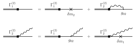
Figure 5: System of equations for the vertex functions in the two-body approximation.

In this approximation, the vertex function $\Gamma_{2}^{\mu}$ is a constant matrix proportional to $\gamma^{\mu}$. With these results, one can calculate the norms of the Fock sectors entering into the normalization condition (23):

$$I_{1} = 4m^{2}\psi_{1}^{2},$$ (44)

$$I_{2} = 4m^{2}\psi_{1}^{2}\,e_{02}^{2}\,J_{2},$$ (45)

where the expression for $J_{2}$ can be found in kms_04 . It depends logarithmically on the mass of the PV boson used to regularize the loop integral. The normalization condition thus fixes $\psi_{1}$:

$$4m^{2}\psi_{1}^{2}=\frac{1}{1+e_{02}^{2}J_{2}}.$$ (46)

The renormalization condition (32) enables us to calculate $e_{02}$ as a function of the physical coupling constant denoted by $e$. This condition, for $N=2$, writes simply

$$\Gamma_{2}^{\mu}=e\gamma^{\mu}\equiv 2e_{02}m\psi_{1}\gamma^{\mu},$$ (47)

since $I_{1}^{(1)}=1$. With Eq. (46) we get

$$e_{02}^{2}=\frac{e^{2}}{1-e^{2}J_{2}}$$ (48)

and

$$I_{1} = 1-e^{2}J_{2},$$ (49)

$$I_{2} = e^{2}J_{2}.$$ (50)

With all these quantities, one can easily calculate the electromagnetic form factors given by the diagrams shown in Fig. 6. Note that since the state vector is normalized to $1$, we find for the external bare coupling constant:

$$\bar{e}_{01}=\bar{e}_{02}=e.$$ (51)

At zero momentum transfer, the Pauli form factor gives the anomalous magnetic moment of the electron. We get kms_08

$$F_{2}(0)=\frac{\alpha}{2\pi}.$$ (52)

This expression exactly coincides with the well-known Schwinger term. One may wonder why our nonperturbative approach exactly recovers the perturbative result ch_09 . The reason is simple. For the two-body Fock space truncation we consider here, the irreducible contributions to the two-point Green’s function or to the electromagnetic form factors are just identical to the corresponding ones in the second order of perturbation theory. And their re-summation to all orders of the coupling constant just defines the physical mass of the electron, which is also the same, by construction, in both approaches.

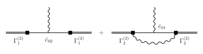
Figure 6: Fermion-boson 3PGF in the two-body approximation.

Our result (52) is also independent of the PV fermion and boson masses, when they tend to infinity. This is of course necessary in order to preserve the scale invariance of physical observables. Note that at large enough PV masses, the one-body part $I_{1}$ of the normalization condition is negative, while the two-body part $I_{2}$ exceeds $1$. This implies also that $e_{02}^{2}$ is negative. These features are just an artefact of the regularization scheme which is used. They show that indeed $I_{1}$ and $I_{2}$, and, more generally, any $I_{n}$ in Eq. (23), as well as the bare coupling constants, are not physical observables and can therefore be scale dependent.

4.3 Scalar system in the three-body approximation: the role of antiparticles

Finding the state vector for the three-body Fock space truncation is the first non-trivial nonperturbative calculation. We begin our consideration of the three-body approximation with the study of a toy model: a heavy scalar boson $B$ with mass $m$, interacting with light scalar bosons $b$ with mass $\mu$. We will calculate the state vector of the heavy boson and represent the former as a sum of the following Fock sectors, in symbolic form:

$$\phi(p)=|B\rangle+|Bb\rangle+|Bbb\rangle+|BB\bar{B}\rangle,$$ (53)

where $\bar{B}$ denotes the antiparticle. The interaction Hamiltonian is

$$H^{int}(x)=-g_{0}B^{2}(x)b(x)-\delta m^{2}B^{2}(x)-\delta\mu^{2}b^{2}(x),$$ (54)

where $\delta m^{2}$ and $\delta\mu^{2}$ are the mass counterterms which, in this model, have the dimension of mass squared. Since the physical coupling constant $g$ has the dimension of mass, it is convenient to define a dimensionless coupling constant $\alpha=g^{2}/16\pi m^{2}$.

The system of eigenstate equations for the vertex functions is represented graphically in Fig. 7. The two three-body vertices $\Gamma_{3}^{(3)}$ and $\Gamma_{3a}^{(3)}$ are trivially expressed through the two-body vertex $\Gamma_{2}^{(3)}$. Due to this fact, we can obtain a closed equation involving $\Gamma_{2}^{(3)}$ only.

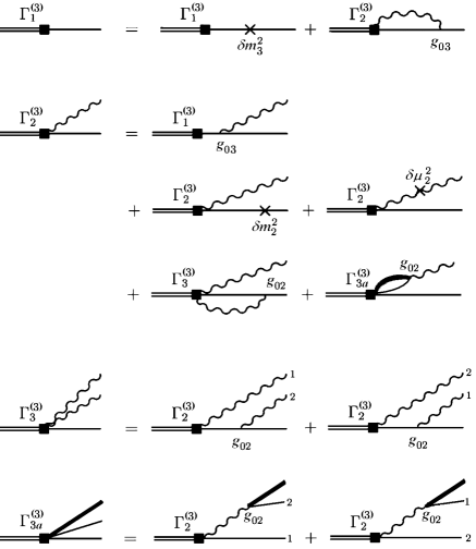
Figure 7: System of equations for the vertex functions of the scalar system in the three-body approximation. The thin and thick ordinary lines stand for heavy bosons and antibosons, respectively. The wavy lines denote light bosons.

In this model, we encounter two types of irreducible divergent contributions: the heavy and light boson self-energies, as shown in Fig. 8. Both of them diverge logarithmically at high momenta; the divergences are expected to be cancelled by the corresponding mass counterterms.

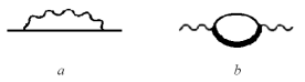
Figure 8: Divergent contributions in the scalar model: the heavy (a) and light (b) boson self energies.

The renormalization condition should now incorporate the light boson field strength normalization factor. Instead of Eq. (32), we have

$$\Gamma_{2}^{(3)}(s_{2}=M^{2})=g\sqrt{Z_{Bb}},$$ (55)

where the factor $Z_{Bb}$ stands for the combined contribution of the heavy and light boson strength normalization factors, calculated according to the FSDR prescription, extended to include antiparticle degrees of freedom kms_10 . This factor is completely finite in a pure scalar system, and is expressed in terms of derivatives of the heavy and light boson self-energies.

The eigenstate equation for $\Gamma_{2}^{(3)}$ with the renormalization condition (55) has been solved numerically in the limit $M\to m$ for the following set of parameters: $m=0.95$, $\mu=0.15$, $\alpha=2$. Note that this value of $\alpha$ is far from the perturbative domain. For convenience, $\Gamma_{2}^{(3)}$ is parameterized as a function of two variables, $s_{2}$ and $x$. The physical domain corresponds to $s_{2}\geq(m+\mu)^{2}$, $0<x<1$. The renormalization point is defined by $s_{2}=m^{2}$ and $x=x^{*}$, where we chose $x^{*}=\mu/(m+\mu)$.

We show in Fig. 9 the characteristic dependence of $\Gamma_{2}^{(3)}$ on one of its arguments, while the second argument is fixed. In contrast to the two-body case, where $\Gamma_{2}^{(2)}$ is a constant, now it exhibits rather nontrivial behavior, especially as a function of $s_{2}$ at fixed $x$.

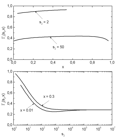
Figure 9: Two-body vertex function in the scalar model as a function of $x$ at fixed $s_{2}$ (upper plot) and as a function of $s_{2}$ at fixed $x$ (lower plot).

To check the consistency of the renormalization condition (55), we show in Fig. 10 the dependence of $\Gamma_{2}^{(3)}$ on $x$ at fixed $s_{2}=m^{2}$. It is distinctly seen that if the Fock space includes all the four Fock sectors, Eq. (53), $\Gamma_{2}^{(3)}(s_{2}=m^{2},x)$ is almost a constant, as it ought to be. If one however neglects one of the three-body sectors, either $|BB\bar{B}\rangle$ or $|Bbb\rangle$, $\Gamma_{2}^{(3)}(s_{2}=m^{2},x)$ strongly depends on $x$, which makes the renormalization condition ambiguous because physical results turn out to be sensitive to the choice of $x^{*}$.

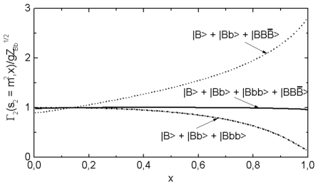
Figure 10: Two-body vertex function (in units of $g\sqrt{Z_{Bb}}$) at $s_{2}=m^{2}$ as a function of $x$. The solid line is the calculation with all the four Fock sectors, Eq. (53), in the state vector. The dash-dotted and dotted lines are the same but without the $|BB\bar{B}\rangle$ or $|Bbb\rangle$ sector, respectively.

The above result is very non-trivial. Let us consider, for instance, a part of the three-body contributions to $\Gamma_{2}^{(3)}$ calculated in perturbation theory, i.e. in terms of the two-body vertex function $\Gamma_{2}^{(2)}$ found in the lower, two-body, approximation, as shown in Fig. 11. Their sum (but not each of them!) is exactly $x$-independent at $s_{2}=m^{2}$, since $\Gamma_{2}^{(2)}$ is a constant. This statement follows from the fact that the sum of the two contributions on the energy shell coincides with the corresponding on-mass-shell Feynman amplitude, and the latter is a constant. In our calculation of order $N=3$, the contributions analogous to those in Fig. 11, but with $\Gamma_{2}^{(3)}$ instead of $\Gamma_{2}^{(2)}$ appear in the eigenstate equation and determine the $x$-dependence of $\Gamma_{2}^{(3)}(s_{2}=m^{2})$. From Fig. 10 it is seen that the latter dependence is surprisingly weak, though $\Gamma_{2}^{(3)}$ is not a constant, as Fig. 9 clearly demonstrates. At the same time, if one calculates the amplitudes of the diagrams in Fig. 11 with an arbitrary chosen function $\Gamma_{2}(s_{2},x)$ instead of $\Gamma_{2}^{(2)}$, their sum would hardly be a constant at $s_{2}=m^{2}$. Such a result may indicate that the set of contributions we considered in the case of the three-body Fock space truncation forms an almost consistent set, in the sense that it meets all consistency requirements. This constitutes a basis of a well-controlled, nonperturbative Fock expansion of the the state vector, in the same spirit as an expansion in $g^{2}$ in perturbation theory.

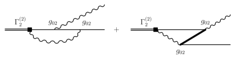
Figure 11: Part of the three-body Fock sector contributions to the two-body vertex.

4.4 Yukawa model in the three-body approximation: calculation of the fermion anomalous magnetic moment

The Yukawa model is much closer to reality (e.g. for instance to QED) than the scalar model discussed in the previous section. Simultaneously, it is much more involved from the point of view of renormalization, because of complicated spin structure of the vertex functions and stronger divergences to be regularized and renormalized. In this section, we apply our FSDR renormalization scheme to the Yukawa model within the three-body Fock space truncation, but, in order to avoid extra complications, without incorporating antifermion degrees of freedom. Our purpose is to demonstrate the capabilities of the FSDR scheme in solving a true nonperturbative problem for particles with spin. For example, in contrast to the two-body Fock space truncation (in this approximation the Yukawa model is almost equivalent to QED, as considered in Sec. 4.2), where we have only one irreducible contribution to the fermion self-energy, we now should consider all the graphs for the self-energy, which contain one fermion and two bosons in intermediate states, including overlapping self-energy type diagrams. The number of such irreducible graphs is infinite. Some of them are shown in Fig. 12. The solution of the eigenstate equation for the state vector automatically generates these contributions to all orders of the coupling constant.

Figure 12: Radiative corrections to the self-energy.

We start with the following Fock decomposition for the state vector

$$\phi(p)=|F\rangle+|Fb\rangle+|Fbb\rangle,$$ (56)

where the symbols $F$ and $b$ denote, respectively, the constituent fermion and boson with masses $m$ and $\mu$. The interaction Hamiltonian reads

$$H^{int}(x)=-g_{0}\bar{\psi}\psi\varphi-\delta m\bar{\psi}\psi-\delta\mu^{2}\varphi^{2}+\delta{H}^{int}_{\omega},$$ (57)

where $\delta{H}^{int}_{\omega}$ is defined by Eq. (33). The regularization is done in a rotationally invariant way by introducing one PV fermion with mass $m_{1}$ and one PV boson with mass $\mu_{1}$.

The system of equations for the vertex functions in graphical representation can be obtained from that for the scalar case, shown in Fig. 7, by changing $\delta m_{2,3}^{2}\to\delta m_{2,3}$, $g_{03}\to g_{03}+Z_{\omega}m{\not\!\omega}/\omega\makebox[2.27626pt]{$\cdot$}p$ and by setting $\delta\mu^{2}_{2}\equiv 0$, $\Gamma_{3a}^{(3)}\equiv 0$, since we do not consider here the dressing of the boson line. After that, the expressions for the light-front diagrams are written according to the CLFD graph technique rules, taking into account that certain lines correspond now to a particle with spin 1/2.

Expressing $\Gamma_{3}^{(3)}$ through $\Gamma_{2}^{(3)}$, as in the scalar case, we get a closed matrix equation for the two-body vertex. Its spin structure is written similarly to Eq. (29):

$$\Gamma_{2}^{(3)}=\bar{u}(k_{1})\left[b_{1}+b_{2}\frac{m{\not\!\omega}}{\omega\makebox[2.27626pt]{$\cdot$}p}\right]u(p),$$ (58)

where $b_{1}$ and $b_{2}$ are scalar functions. For clarity, we indicate here only the physical components. The PV fermion and boson components can be calculated as well yukawa .

The three-body component is completely determined by four scalar functions, like, for instance

$$\bar{u}(k_{1})\Gamma_{3}^{(3)}(1,2,3)u(p)$$ (59)

$$=\bar{u}(k_{1})\Bigl{(}g_{1}\,S_{1}+g_{2}\,S_{2}+g_{3}\,S_{3}+g_{4}\,S_{4}\Bigr{)}u(p),$$

where these functions are denoted $g_{1-4}$, and $S_{1-4}$ are basis spin structures. It is convenient to construct the the latter ones as follows karm98 :

$$S_{1} = 2x_{1}-(1+x_{1})\displaystyle{\frac{m\not\!\omega}{\omega\makebox[2.27626pt]{$\cdot$}p}},$$

$$S_{2} = \displaystyle{\frac{m\not\!\omega}{\omega\makebox[2.27626pt]{$\cdot$}p}},$$

$$S_{3} = iC_{ps}\left[2x_{1}-(1-x_{1})\displaystyle{\frac{m\not\!\omega}{\omega\makebox[2.27626pt]{$\cdot$}p}}\right]\gamma_{5},$$

$$S_{4} = i\,C_{ps}\displaystyle{\frac{m\not\!\omega}{\omega\makebox[2.27626pt]{$\cdot$}p}}\gamma_{5}$$ (60)

with $x_{1}=\frac{\omega\makebox[2.27626pt]{$\cdot$}k_{1}}{\omega\makebox[2.27626pt]{$\cdot$}p}$, while $C_{ps}$ is the following pseudoscalar:

$$C_{ps}=\frac{1}{m^{2}\omega\makebox[2.27626pt]{$\cdot$}p}e^{\mu\nu\rho\gamma}k_{2\mu}k_{3\nu}p_{\rho}\omega_{\gamma}.$$ (61)

The function $C_{ps}$ can only be constructed with four independent four-vectors. This is the case in LFD for $n\geq 3$. In the nonrelativistic limit, one would need $n\geq 4$. We can then construct two additional spin structures $S_{3}$ and $S_{4}$ of the same parity as $S_{1}$ and $S_{2}$ by combining $C_{ps}$ with parity negative matrices constructed from $S_{1}$, $S_{2}$, and $\gamma_{5}$ matrices.

In our computational procedure we take the limit $m_{1}\to\infty$ analytically and then study the limit $\mu_{1}\to\infty$ numerically. As a result, the calculated vertex functions depend parametrically on $\mu_{1}$. The main question we are interested in concerns the behavior of observables as a function of $\mu_{1}$: do they remain finite and physically reasonable at $\mu_{1}\to\infty$ or not? For this purpose, we calculate the fermion anomalous magnetic moment, using the state vector (56). It can be extracted from the fermion-boson 3PGF in the three-body approximation, as shown in Fig. 13. The detail of the calculation can be found in yukawa . We just recall here the main numerical results.

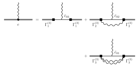
Figure 13: Fermion-boson 3PGF in the three-body approximation.

The anomalous magnetic moment is calculated for a typical set of physical parameters $m=0.938$ GeV, $\mu=0.138$ GeV, and two values of the coupling constant $\alpha\equiv\frac{g^{2}}{4\pi}=0.2$ and $0.5$. This mimics, to some extent, a physical nucleon coupled to scalar ”pions”. The typical pion-nucleon coupling constant is given by $g=\frac{g_{A}}{2F_{\pi}}\langle k\rangle$ where $\langle k\rangle$ is a typical momentum scale, and $g_{A}$ and $F_{\pi}$ are the axial coupling constant and the pion decay constant, respectively. For $\langle k\rangle=0.2$ GeV we just get $\alpha\simeq 0.2$.

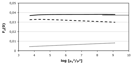
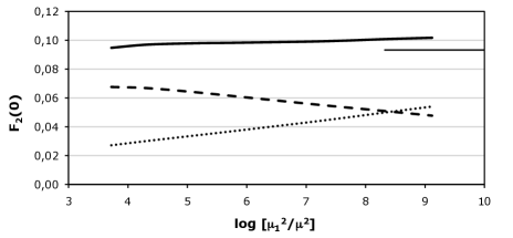
Figure 14: The anomalous magnetic moment in the Yukawa model as a function of the PV mass $\mu_{1}$, for two different values of the coupling constant, $\alpha=0.2$ (upper plot) and $0.5$ (lower plot). The dashed and dotted lines are, respectively, the two- and three-body contributions, while the solid line is the total result. The value of the anomalous magnetic moment calculated in the $N=2$ approximation is shown by the thin line on the right axis.

We plot in Fig. 14 the anomalous magnetic moment as a function of $\log\left[\frac{\mu_{1}^{2}}{\mu^{2}}\right]$, for the two different values of $\alpha$ mentioned above. We show also on each of these plots the value of the anomalous magnetic moment calculated for the $N=2$ truncation, which coincides with the anomalous magnetic moment obtained in the second order of perturbation theory. The results for $\alpha=0.2$ show rather good convergence as $\mu_{1}\to\infty$. The contribution of the three-body Fock sector to the anomalous magnetic moment is sizeable but small, indicating that the Fock decomposition (16) converges rapidly. This may show that once higher Fock components are small, we can achieve a practically converging calculation of the anomalous magnetic moment. Note that this value of $\alpha$ is not particularly small: it is about 30 times the electromagnetic coupling, and is about the size of the typical pion-nucleon coupling in a nucleus.

When $\alpha$ increases, we see that the contribution of the three-body sector considerably increases. For $\alpha=0.5$ the three-body contribution to the anomalous magnetic moment starts to dominate at large values of $\mu_{1}$. The dependence of the anomalous magnetic moment on the PV boson mass $\mu_{1}$ becomes more appreciable, although it keeps rather small.

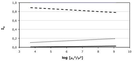
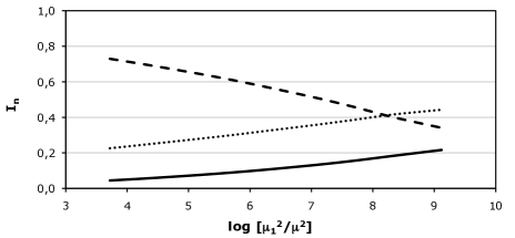
Figure 15: Individual contributions of the one- (dashed line), two- (dotted line), and three-body (solid line) Fock sectors to the norm, fixed to $1$, of the state vector, as a function of the PV boson mass $\mu_{1}$, for $\alpha=0.2$ (upper plot) and $\alpha=0.5$ (lower plot).

In order to have a more physical insight into the relative importance of different Fock sectors in the decomposition (16) for the state vector, we plot in Fig. 15 the contributions of the one-, two-, and three-body Fock sectors to the norm of the state vector for the two values of the coupling constant, considered in this work. We see again that at $\alpha=0.2$ the three-body contribution to the norm is small, while it is not negligible and increases with $\mu_{1}$, when $\alpha=0.5$.

According to renormalization theory, the PV boson mass should be much larger than any intrinsic momentum scale present in the calculation of physical observables. With this limitation, physical observables should be independent of any variation of the PV boson mass, within an accuracy which can be increased at will. This is what we found in our numerical calculation for small enough values of $\alpha$.

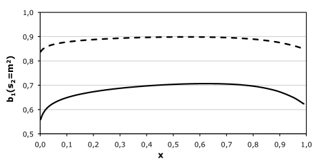
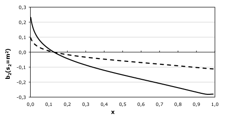
Figure 16: The spin components $b_{1}$ (upper plot) and $b_{2}$ (lower plot) of the two-body vertex function calculated at $s_{2}=m^{2}$, as a function of $x$, for $\alpha=0.2$ (dashed line) and $\alpha=0.5$ (solid line), for a typical value of $\mu_{1}=100$ GeV.

In order to understand the possible origin of the residual dependence of the anomalous magnetic moment on $\mu_{1}$, we plot in Figs. 16 the two-body spin components $b_{1}$ and $b_{2}$ calculated at $s_{2}=m^{2}$, as a function of $x$. As we already mentioned in Sec. 3.3, the spin components for physical particles $b_{1}(s_{2}=m^{2})$ and $b_{2}(s_{2}=m^{2})$ should be independent of $x$ in an exact calculation. Moreover, $b_{2}(s_{2}=m^{2})$ should be zero. It is here fixed to zero at a given value of $x=x^{*}\equiv\frac{\mu}{m+\mu}$, by the adjustment of the constant $Z_{\omega}$. We clearly see in these plots that the on-shell $b_{1}$ is not a constant, although its dependence on $x$ is always weak, while $b_{2}$ is not identically zero, although its value is relatively smaller than that of $b_{1}$ for $\alpha=0.2$, and starts to be not negligible for $\alpha=0.5$. A similar situation is observed in the scalar case, when we remove ”by hands”, from the state vector, the Fock sector with the antiparticle (see the dash-dotted curve in Fig. 10).

It is instructive to study the properties of $b_{1,2}(s_{2}=m^{2})$ in perturbation theory. This can be done by calculating the amplitudes of the diagrams shown in Fig. 11 (but for fermions, of course!). Note that in our Fock space truncation (56), the contribution of the $Fbb$ intermediate state (the left diagram in Fig. 11) is automatically taken into account by the solution of the eigenstate equation, while the contribution of the $FF\bar{F}$ state (the right diagram in the same figure) is absent. If one calculates the sum of both contributions within perturbation theory kms09 , one finds

$$b_{1}^{pert}(s_{2}=m^{2}) = const,$$ (62)

$$b_{2}^{pert}(s_{2}=m^{2}) = 0.$$ (63)

This is a first indication that the expected properties of the on-shell functions $b_{1,2}$ are indeed recovered, when antifermion degrees of freedom are involved. This is also a confirmation of similar features found in Sec. 4.3 for the scalar system.

4.5 Light-front chiral effective field theory

The calculation of baryon properties within the framework of chiral perturbation theory is a subject of active theoretical developments. Since the nucleon mass is not zero in the chiral limit, all momentum scales are a priori involved in the calculation of baryon properties (like masses or electro-weak observables) beyond tree level. This is at variance with the meson sector for which a meaningful power expansion of any physical amplitude can be done.

While there is not much freedom, thanks to chiral symmetry, for the construction of the effective Lagrangian in chiral perturbation theory in terms of the pion field — or more precisely in terms of the U field defined by $U=e^{i{\bf\tau}.{\bf\pi}/f_{\pi}}$, where $f_{\pi}$ is the pion decay constant and $\tau$ are the Pauli matrices, — one should settle an appropriate approximation scheme in order to calculate baryon properties. Up to now, two main strategies have been adopted. The first one is to force the bare (and hence the physical) nucleon mass to be infinite, in heavy baryon chiral perturbation theory manohar . In this case, by construction, an expansion in characteristic momenta can be developed. The second one is to use a specific regularization scheme IR in order to separate contributions which exhibit a meaningful power expansion, and hide the other parts in appropriate counterterms. In both cases however, the explicit calculation of baryon properties relies on an extra approximation in the sense that physical amplitudes are further calculated by expanding the effective Lagrangian, denoted by ${\cal L}_{CPT}$, in a finite number of pion fields.

Moreover, it has recently been realized that the contribution of pion-nucleon resonances, like the $\Delta$ and Roper resonances, may play an important role in the understanding of the nucleon properties at low energies delta . These resonances are just added ”by hand” in the chiral effective Lagrangian. This is also the case for the most important $2\pi$ resonances, like the $\sigma$ and $\rho$ resonances.

Since in the chiral limit the pion mass is zero, any calculation of $\pi N$ systems demands a relativistic framework to get, for instance, the right analytical properties of the physical amplitudes. The calculation of compound systems, like a physical nucleon composed of a bare nucleon coupled to many pions, relies also on a nonperturbative eigenstate equation. While the mass of the system can be determined in leading order from the iteration of the $\pi N$ self-energy calculated in the first order of perturbation theory, as indicated in Fig. 17(a), this is in general not possible, in particular, for $\pi N$ irreducible contributions, as shown in Fig. 17(b).

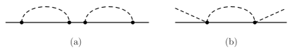
Figure 17: Iteration of the self-energy contribution in the first order of perturbation theory (a); irreducible contribution to the bound state equation (b). Dashed lines represent pions.

The general framework we have developed above is particularly suited to deal with these requirements. This leads to the formulation of light-front chiral effective field theory (LF$\chi$EFT) LF_jf with a specific effective Lagrangian ${\cal L}_{eff}$. The decomposition of the state vector in a finite number of Fock components implies to consider an effective Lagrangian which enables all possible elementary couplings between the pion and nucleon fields compatible with the Fock space truncation. This is indeed easy to achieve in chiral perturbation theory, since each derivative of the U field involves one derivative of the pion field. In the chiral limit, the chiral effective Lagrangian of order $p$, ${\cal L}_{CPT}^{p}$, involves $p$ derivatives and therefore at least $p$ degrees of the pion field. In order to calculate the state vector in the $N$-body approximation, with one fermion and $(N-1)$ pions, one has therefore to include contributions up to $2(N-1)$ pion fields in the effective Lagrangian, as shown in Fig. 18. We thus should calculate the state vector in the $N$-body approximation with an effective Lagrangian denoted by ${\cal L}_{eff}^{N}$ and given by

$${\cal L}_{eff}^{N}={\cal L}_{CPT}^{p=2(N-1)}\ .$$ (64)

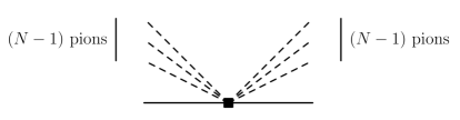
Figure 18: General vertex including a maximum of $(N-1)$ pion fields in the initial and final states.

While the effective Lagrangian in LF$\chi$EFT can be mapped out to the CPT Lagrangian of order $p$, the calculation of the state vector does not rely on any momentum decomposition. It relies only on an expansion in the number of pions in flight at a given light-front time. In other words, it relies on an expansion in the fluctuation time, $\tau_{f}$, of such a contribution. From general arguments, the more particles we have at a given light-front time, the smaller the fluctuation time is. At low energies, when all processes have characteristic interaction times larger than $\tau_{f}$, this expansion should be meaningful.

It is interesting to illustrate the general features of LF$\chi$EFT calculations. At order $N=2$, we already have to deal with irreducible contributions, as shown in Fig. 17(b). It leads to non-trivial renormalization of the coupling constant. The calculation at order $N=3$ incorporates explicitly contributions coming from $\pi\pi$ interactions, as well as all low energy $\pi N$ resonances, like the $\Delta$ or Roper resonances, as shown schematically in Fig. (19). Indeed, in the $|\pi\pi N\rangle$ Fock sector, the $\pi N$ state can couple to both $J=T=3/2$ as well as $J=T=1/2$ states. We can generate therefore all $\pi N$ resonances in the intermediate state without the need to include them explicitly, provided the effective Lagrangian has the right dynamics to generate these resonances. This is the case, by the construction, in CPT.

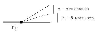
Figure 19: Three-body vertex function which exhibits both the contribution of $2\pi$ resonances and $\Delta$ as well as Roper nucleon resonances.

Preliminary results obtained by using the PV regularization scheme can be found in LF_kmt .

5 Conclusion and perspectives

The understanding of the properties of relativistic compound systems from an elementary Hamiltonian in nuclear and particle physics demands to develop a nonperturbative framework. This framework should include a well-defined strategy for approximate calculations of these properties and a systematic way to improve the accuracy.

We have described in this review a general framework based on light-front dynamics. In this scheme, the state vector of any system of interacting particles is decomposed in Fock components. Since for obvious practical reasons this decomposition should be truncated to take into account a finite number of Fock components, we have shown how to control in a systematic way the convergence of such expansion.

Our formalism relies, first, on the covariant formulation of light-front dynamics, and, second, on a systematic nonperturbative renormalization scheme in order to avoid any uncancelled divergences. The applications we have presented on QED, on a purely scalar system, on the Yukawa model, and on chiral effective field theory on the light-front have shown the flexibility, the real advantages, and the nice features of our formalism.

Several developments will soon achieve to settle a complete framework to deal with field theory on the light front. This includes first the full account of antiparticle degrees of freedom in order to recover, order by order in the Fock expansion, the scale invariance of physical observables for arbitrary values of the coupling constant. This scale invariance should be checked within a given regularization scheme.

We have used up to now the Pauli-Villars regularization scheme. While this scheme is systematic and can be applied to a variety of physical systems, it may be cumbersome to implement from a numerical point of view in higher order calculations, since it involves many non-physical components including Pauli-Villars fields. It also demands to perform calculations with very large mass scales (the Pauli-Villars fermion and boson masses). The use of the Taylor-Lagrange renormalization scheme TLRS has proven to be a very natural scheme in light-front dynamics. It should be applied to more involved calculations.

Finally, it is now well-recognized that the understanding of spontaneous symmetry breaking phenomena on the light-front can be achieved by taking into account nonperturbative zero mode contributions to field operators hksw . It remains to include these zero modes in the general framework we developed in this review.