On Possible Implications of Self-Organization Processes through
Transformation of Laws of Arithmetic into Laws of Space and Time

Abstract

In the paper we present results based on the description of complex systems in terms of self-organization processes of prime integer relations. Realized through the unity of two equivalent forms, i.e., arithmetical and geometrical, the description allows to transform the laws of a complex system in terms of arithmetic into the laws of the system in terms of space and time. Possible implications of the results are discussed.

I Introduction

In the paper we present results based on the description of complex systems in terms of self-organization processes of prime integer relations and discuss their possible implications.

Rather than space and time, the description suggests a new stage for understanding and dealing with complex systems, i.e., the hierarchical network of prime integer relations. It appears as the structure built by the totality of the processes and existing through the mutual consistency of its parts. Based on the integers and controlled by arithmetic only the description can picture complex systems by irreducible concepts alone and thus secure its foundation. Remarkably, this raises the possibility to develop an irreducible theory of complex systems Korotkikh_1 -Korotkikh_9 .

In section II we give some basics of the description to present its two equivalent forms and show that the description can work arithmetically and geometrically all at once.

In the arithmetical form a complex system is characterized by hierarchical correlation structures determined by self-organization processes of prime integer relations. The correlation structures operate through the relationships emerging in the formation of the prime integer relations. Since a prime integer relation expresses a law between the integers, the complex system is, in fact, governed by the laws of arithmetic realized through the self-organization processes of prime integer relations.

In the geometrical form the correlation structures of the complex system are given by hierarchical structures of two-dimensional geometrical patterns, as the processes become isomorphically expressed in terms of their transformations. This geometrizes the correlations as well as the laws of arithmetic the complex system is determined by. As a result, the geometrization gives the body to the correlations and to the laws of arithmetic to be characterized by space and time as dynamics variables. This allows to transform the laws of the complex system in terms of arithmetic into the laws of the system in terms of space and time.

To have a picture of the hierarchical network in section III we consider a process that can probe the hierarchical network on all levels.

In section IV we discuss a scale-invariant property of the process suggesting its effective representation, where the levels are arranged into the groups of three successive levels with important consequences. In particular, by using renormalizations in such a group the process can be given by a series of approximations so that the first term characterizes the process in a self-similar way to the characterization at levels $1,2$ and $3$.

Consequently, the process at these three levels provides a first resolution picture of the hierarchical network, where the correlation structure determined by the process is isomorphically represented by a hierarchical structure of two-dimensional geometrical patterns.

In section V we analyze the picture in more detail and represent the hierarchical structure of geometrical patterns by using space and time as dynamical variables. This allows to transform the laws of the process in terms of arithmetic into the laws in terms of space and time. As a result, local spacetimes of the elementary parts become defined and we can consider how they appear to be related to one another.

Remarkably, in the representation the elementary parts of the correlation structure act as the carriers of the laws of arithmetic with each elementary part carrying its own quantum of the laws. This opens an important perspective to use elementary parts as quanta to construct different laws and in section VI we consider how the laws of arithmetic could be transformed into different forms by constructing global spacetimes.

In section VII we discuss possible implications of the results.

II Basics of the Description

The description of complex systems in terms of self-organization processes of prime integer relations is realized through the unity of two equivalent forms, i.e., arithmetical and geometrical Korotkikh_1 -Korotkikh_9 .

In particular, in the geometrical form $N\geq 2$ elementary parts $P_{10},...,P_{N0}$ as the initial building blocks in the formation of a complex system are considered at level $0$. An elementary part $P_{j0},j=1,...,N$ is given through a local reference frame specified by two parameters $\delta_{j}>0$ and $\varepsilon_{j}>0$. The local reference frame is a setting to characterize the elementary part $P_{j0}$ and accommodate the changes determined by the formation. The reference frames are arranged to consider the elementary parts $P_{10},...,P_{N0}$ simultaneously, yet each in its own reference frame without information about the distances in space and time.

The geometrical form requires the parameters to be the same

$$\delta=\delta_{j},\ \ \ \varepsilon=\varepsilon_{j},\ \ \ j=1,...,N,$$

which are associated with dimensionless quantities of space and time

$$\delta=\frac{\chi_{0}}{\chi_{min}},\ \ \ \varepsilon=\frac{\tau_{0}}{\tau_{min}},$$

where $\chi_{0}$ and $\tau_{0}$ are the length scales of space and time at level $0$, and $\chi_{min}$ and $\tau_{min}$ are corresponding minimum length scales.

Since

$$\chi_{0}\geq\chi_{min},\ \ \ \tau_{0}\geq\tau_{min},$$

we have

$$\delta\geq 1,\ \ \ \varepsilon\geq 1.$$ (1)

In general, the parameters $\delta$ and $\varepsilon$ give us a choice in setting the geometrical form and become the basic constants, which can not be changed unless in all reference frames of the elementary parts.

The state of an elementary part $P_{j0},j=1,...,N$ is determined to characterize the geometry of a corresponding self-organization process of prime integer relations at level $0$. In particular, the state of the elementary part $P_{j0}$ can be given by the space coordinate $X_{j0}=s_{j}\delta$, while the time coordinate $T_{j0}$ changes independently by $\varepsilon$, where $s_{j}\in I$ and $I$ is a set of integers. The state of the elementary parts $P_{10},...,P_{N0}$ can be specified by a sequence

$$s=s_{1}...s_{N}\in I_{N},$$

where $I_{N}$ is a set of sequences of length $N$, and represented by a piecewise constant function.

In particular, let

$$\rho_{m\varepsilon\delta}:s\rightarrow f$$

be a mapping that associates a sequence $s=s_{1}...s_{N}\in I_{N}$ with a function $f$, denoted $f=\rho_{m\varepsilon\delta}(s)$, such that

$$f(t)=s_{j}\delta,\ \ \ t\in[t_{m+j-1},t_{m+j}),\ \ \ j=1,...,N,$$

$$f(t_{m+N})=s_{N}\delta,\ \ \ t_{j}=j\varepsilon,\ \ \ j=m,...,m+N$$

and

$$f^{[j]}(t_{m})=0,\ \ \ j=1,2,...\ ,$$

where $m$ is an integer.

Let

$$I_{N}(Q_{1},...,Q_{k})\subset I_{N}$$

be the states of the elementary parts $P_{10},...,P_{N0}$ such that if

$$s=s_{1}...s_{N}\in I_{N}(Q_{1},...,Q_{k})$$

and

$$s^{\prime}=s_{1}^{\prime}...s_{N}^{\prime}\in I_{N}(Q_{1},...,Q_{k}),$$

then

$$Q_{j}=f^{[j]}(t_{m+N})=g^{[j]}(t_{m+N}),\ \ \ j=1,...,k,$$

but

$$f^{[k+1]}(t_{m+N})\neq g^{[k+1]}(t_{m+N}),$$

where $f^{[j]}(t)$ and $g^{[j]}(t),\ t\in[t_{m},t_{m+N}],\ j=1,...,k+1$ are the $j$th integrals of the functions $f=\rho_{m\varepsilon\delta}(s)$ and $g=\rho_{m\varepsilon\delta}(s^{\prime})$ accordingly.

Importantly, the quantities $Q_{1},...,Q_{k}$ can define a complex system and its formation from the elementary parts $P_{10},...,P_{N0}$ Korotkikh_1 -Korotkikh_6 . In particular, the states $I_{N}(Q_{1},...,Q_{k})$ of the elementary parts $P_{10},...,P_{N0}$ can determine the states of the system with the transitions preserving the quantities $Q_{1},...,Q_{k}$ and thus the system itself. Since a system can be in one of the possible states, it is not possible to predict which state will be actually measured in any given case and thus the description provides the statistical information about the system.

The integer code series Korotkikh_1 , as the origin of the description, plays a crucial role. In fact, it is the key to prove that in the transition between two states

$$s=s_{1}...s_{N}\in I_{N}(Q_{1},...,Q_{k})$$

and

$$s^{\prime}=s_{1}^{\prime}...s_{N}^{\prime}\in I_{N}(Q_{1},...,Q_{k})$$

of the elementary parts $P_{10},...,P_{N0}$ the $Q_{1},...,Q_{k}$ quantities remain invariant

$$Q_{j}=f^{[j]}(t_{m+N})=g^{[j]}(t_{m+N}),\ \ \ j=1,...,k,$$ (2)

but

$$f^{[k+1]}(t_{m+N})\neq g^{[k+1]}(t_{m+N}),$$

if and only if the correlations between the parts in the formation of the system are defined by $k$ Diophantine equations

$$(m+N)^{k-1}\Delta s_{1}+...+(m+1)^{k-1}\Delta s_{N}=0$$

$$.\qquad\qquad.\qquad\qquad.\qquad\qquad.\qquad\qquad.$$

$$(m+N)^{1}\Delta s_{1}+...+(m+1)^{1}\Delta s_{N}=0$$

$$(m+N)^{0}\Delta s_{1}+...+(m+1)^{0}\Delta s_{N}=0$$ (3)

and an inequality

$$(m+N)^{k}\Delta s_{1}+...+(m+1)^{k}\Delta s_{N}\neq 0,$$ (4)

where $f=\rho_{m\varepsilon\delta}(s),\ g=\rho_{m\varepsilon\delta}(s^{\prime})$ and

$$\Delta s_{1}...\Delta s_{N}=s_{1}^{\prime}-s_{1},...,s_{N}^{\prime}-s_{N}.$$

Significantly, through the analysis of the Diophantine equations $(\ref{SectionII.3})$ and inequality $(\ref{SectionII.4})$ certain hierarchical structures can be revealed and interpreted as a result of self-organization processes of prime integer relations (Figure 1). In fact, the processes give rise to the hierarchical structures of prime integer relations, which entirely determine the correlation structures (Figure 2) in control of the transition of the system Korotkikh_1 -Korotkikh_6 .

The concept of prime integer relation captures that the prime integer relations are built by the processes as indivisible wholes. In particular, a prime integer relation is made by a process first from integers and then prime integer relations from the levels below. Remarkably, all the components of the prime integer relation are necessary and sufficient for the prime integer relation to exist. In other words, a prime integer relation can be seen as a system itself, where each and every part is important for its formation Korotkikh_1 -Korotkikh_6 .

In the description a correlation structure of a complex system is determined by a self-organization process of prime integer relations. In particular, under a self-organization process elementary parts of level $0$ combine into parts of level $1$, which in their turn compose more complex parts of level $2$ and so on. The formation continues as long as the process can provide the relationships for parts to be made. Notably, in the formation an elementary part of a level transforms into an elementary part of a larger part at the higher level.

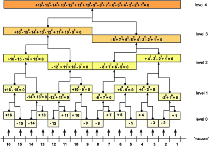
Figure 1: The figure shows a hierarchical structure of prime integer relations, which can be interpreted as a result of a self-organization process. The process starts when integers $16,13,11,10,7,6,4,1$ in the positive state and integers $15,14,12,9,8,5,3,2$ in the negative state are generated from the ”vacuum” to appear at level $0$. The ”vacuum” encodes all possible processes to be realized in the construction of the hierarchical network of prime integer relations. Since a prime integer relation expresses a law between the integers, the structure can be seen as a hierarchical set of laws of arithmetic.

Remarkably, the correlation structures of the transitions entirely define the system. Indeed, they strictly determine the changes between the states so that the quantities and thus the system remain the same. As each of the correlation structures is ready to exercise its own scenario and there is no mechanism specifying which of them is going to take place, an intrinsic uncertainty about the system exists. At the same time the information about the correlation structures can be used to evaluate the probability of a state observable to take each of the possible outcomes.

Importantly, the Diophantine equations $(\ref{SectionII.3})$ have no reference to the distances between the parts in space and time, and thus suggest that the correlations are nonlocal in character. Therefore, according to the description, parts of a complex system may be far apart in space and time and yet remain interconnected with instantaneous effect on each other through the prime integer relations. In fact, through the prime integer relations the elementary parts receive information instantaneously, wherever they happen to be in the correlation structure.

Moreover, since a prime integer relation expresses a law between the integers, consequently, a complex system become governed by the laws of arithmetic realized through the self-organization processes of prime integer relations.

In the geometrical form the correlation structures of a complex system become isomorphically represented by hierarchical structures of two-dimensional patterns Korotkikh_1 -Korotkikh_3 . Importantly, this geometrizes the correlations as well as the laws of arithmetic the complex system is determined by and allows to consider their representations in terms of space and time. As a result, the space and time appear as a manifestation of the prime integer relations and thus the integers Korotkikh_6 -Korotkikh_9 .

Significantly, the geometrization allows to transform the laws of a complex system in terms of arithmetic into the laws of the system in terms of space and time. In particular, this specifies the state of an elementary part at level $0$.

In the arithmetical form a self-organization process starts when integers are generated from the ”vacuum” to appear at level $0$ with an integer in the positive or negative state. As a result, an elementary part, depending on the state of a corresponding integer, becomes positive or negative. At level $0$, where there are no relationships between the integers to provide interactions for the elementary parts, an elementary part is not forced to move and can be defined in the state of rest. In the geometrical form the boundary curve of the two-dimensional pattern of an elementary part at level $0$ is specified by a constant function. Therefore, the boundary curve of the geometrical pattern can be represented by the space coordinate of the elementary part as a constant, given by the value of the function, while the time coordinate can change independently by $\varepsilon$.

Remarkably, the state of an elementary part at level $0$ reveals a parallel with the law of inertia postulated in classical mechanics Galilei_1 -Mach_1 . In our description the state of an elementary part is defined by the laws of arithmetic realized through the processes at level $0$.

Rather than space and time, the description suggests a new stage for understanding and dealing with complex systems, i.e., the hierarchical network of prime integer relations. It appears as the structure built by the totality of the processes and existing through the mutual consistency of its parts Korotkikh_1 -Korotkikh_6 .

In the hierarchical network an event takes place through a correlation structure as a basic causal element, which defines the notion of simultaneity in the description. In particular, once a correlation structure of a complex system turns to be operational, then through the prime integer relations the parts, irrespective of the distances and levels, become all instantaneously connected, and the correlations are simultaneously realized for the geometrical patterns to be in full agreement with the prime integer relations.

Notably, the effect of the correlations on an elementary part is given by its geometrical pattern and can be different for elementary parts. However, for each elementary part it is exactly as required to preserve the system. In particular, in the representation of the correlations with space and time as dynamic variables it may turn out that the clocks of elementary parts tick differently, yet exactly as determined by the prime integer relations Korotkikh_6 -Korotkikh_9 .

Strictly controlled by arithmetic the prime integer relations as well as their geometrical patterns can not be changed even a bit and thus stand as rigid bodies interconnected by the processes. As a result, the hierarchical network can be used as an absolute reference for motion. Namely, in the hierarchical network the position and motion of a complex system can be specified by the processes in control of the correlation structures. Moreover, in space and time the motion of an elementary part relative to this absolute frame of reference can be defined by the representation of the correlations through the geometrical pattern.

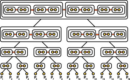
Figure 2: Correlation structure corresponding to the hierarchical structure of prime integer relations. The elementary parts at level $0$ shown as $P_{1},...,P_{16}$ are the initial building blocks in the formation of the hierarchical correlation structure. The structure is built across different levels as under the self-organization process the elementary parts combine into parts, which in their turn compose more complex parts and so on. The formation continues as long as the prime integer relations provide the relationships.

Importantly, based on the integers and controlled by arithmetic only the description can picture complex systems by irreducible concepts alone and thus secure its foundation. This raises the possibility to develop an irreducible theory of complex systems Korotkikh_1 -Korotkikh_9 .

In the next section we consider a process that can probe the hierarchical network on all levels and thus may provide information about it as a whole.

III Making a Picture of the Hierarchical Network

Let us consider a self-organization process of prime integer relations that can determine a correlation structure of a complex system with the changes

$$\Delta s_{1}...\Delta s_{N}=s_{1}^{\prime}-s_{1},...,s_{N}^{\prime}-s_{N}$$

between two states

$$s=s_{1}...s_{N},\ \ \ s^{\prime}=s_{1}^{\prime}...s_{N}^{\prime}$$

of the elementary parts $P_{10},...,P_{N0}$ specified by the PTM (Prouhet-Thue-Morse) sequence

$$\eta=+1-1-1+1-1+1+1-1...=\eta_{1}...\eta_{N}...\ ,$$

where $\Delta s_{j}=\eta_{j},\ j=1,...,N$.

Significantly, as the number $N$ of the elementary parts $P_{10},...,P_{N0}$ increases, the process can probe the hierarchical network on all its levels and, in particular, reach level $log_{2}N$, when $N=2^{k},k=1,2,...\$ Korotkikh_1 . In this case the Diophantine equations $(\ref{SectionII.3})$ and inequality $(\ref{SectionII.4})$ become respectively

$$\eta_{1}N^{k-1}+...+\eta_{N-1}2^{k-1}+\eta_{N}1^{k-1}=0$$

$$.\qquad\qquad.\qquad\qquad.\qquad\qquad.$$

$$\eta_{1}N^{1}+...+\eta_{N-1}2^{1}+\eta_{N}1^{1}=0$$

$$\eta_{1}N^{0}+...+\eta_{N-1}2^{0}+\eta_{N}1^{0}=0$$ (5)

and

$$\eta_{1}N^{k}+...+\eta_{N-1}2^{k}+\eta_{N}1^{k}\neq 0,$$ (6)

where $m=0$. For example, when $N=16$ we can explicitly write down $(\ref{SectionIII.1})$ and $(\ref{SectionIII.2})$ as

$$+16^{3}-15^{3}-14^{3}+13^{3}-12^{3}+11^{3}+10^{3}-9^{3}$$

$$-8^{3}+7^{3}+6^{3}-5^{3}+4^{3}-3^{3}-2^{3}+1^{3}=0$$

$$+16^{2}-15^{2}-14^{2}+13^{2}-12^{2}+11^{2}+10^{2}-9^{2}$$

$$-8^{2}+7^{2}+6^{2}-5^{2}+4^{2}-3^{2}-2^{2}+1^{2}=0$$

$$+16^{1}-15^{1}-14^{1}+13^{1}-12^{1}+11^{1}+10^{1}-9^{1}$$

$$-8^{1}+7^{1}+6^{1}-5^{1}+4^{1}-3^{1}-2^{1}+1^{1}=0$$

$$+16^{0}-15^{0}-14^{0}+13^{0}-12^{0}+11^{0}+10^{0}-9^{0}$$

$$-8^{0}+7^{0}+6^{0}-5^{0}+4^{0}-3^{0}-2^{0}+1^{0}=0$$ (7)

and

$$+16^{4}-15^{4}-14^{4}+13^{4}-12^{4}+11^{4}+10^{4}-9^{4}$$

$$-8^{4}+7^{4}+6^{4}-5^{4}+4^{4}-3^{4}-2^{4}+1^{4}\neq 0.$$

Importantly, the resulting system of integer identities (7) can be seen as a hierarchical set of laws of arithmetic (Figure 1).

The self-organization process starts as integers $N,...,1$ make a transition from the ”vacuum” to level $0$, where each integer acquires the state, positive or negative, depending on the sign of the corresponding element in the PTM sequence. Then the integers combine into pairs and make up the integer relations of level $1$. Following a single organizing principle Korotkikh_1 -Korotkikh_3 the process continues as long as arithmetic allows the integer relations of a level to form the integer relations of the higher level. Notably, in each of the integer relations all components it is made of are necessary and sufficient and this is the reason why we call the integer relations prime.

As long as the integers of level $l=0$ or the prime integer relations of level $l=1,...,k-1$ can form the prime integer relations of level $l+1$, the relationships for the parts of level $l$ to compose the parts of level $l+1$ are provided (Figure 2). As a result, the elementary parts $P_{1l},...,P_{Nl}$ of level $l$ transform to become the elementary parts $P_{1,l+1},...,P_{N,l+1}$ of more complex parts of level $l+1$. Within a part the elementary parts can effect each other through the relationships provided by the prime integer relation thus making the relationships instrumental in the preservation of the part.

Remarkably, in the geometrical form the self-organization process become isomorphically represented by transformations of two-dimensional patterns (Figure 3). In particular, under the isomorphism a prime integer relation turns into the geometrical pattern, which can be viewed as the prime integer relation itself, but only expressed geometrically.

At level $0$ the geometrical patterns corresponding to the integers and the elementary parts $P_{10},...,P_{N0}$ are specified by a piecewise constant function

$$\Psi^{[0]}_{1}=\Psi_{1}=\rho_{0\varepsilon\delta}(\eta),\ \eta\in I_{N}$$

such that

$$\Psi^{[0]}_{1}(t)=\eta_{j}\delta,\ \ \ t_{j-1}\leq t<t_{j},$$

$$t_{j}=j\varepsilon,\ \ \ j=1,...,N.$$

In our description the geometrical pattern of an elementary part $P_{j0},j=1,...,N$ is defined by the region enclosed by its boundary curve, i.e., the graph of the function $\Psi_{1}^{[0]}(t),t_{j-1}\leq t<t_{j}$, the vertical lines $t=t_{j-1},t=t_{j}$ and the $t$-axis. In their turn the space and time coordinates of the elementary part $P_{j0}$ are defined by the representation of the boundary curve of the geometrical pattern.

In particular, in the transition from one state into another at the moment $T_{j0}(t_{j-1})=0$ of the local time the space coordinate $X_{j0}(t_{j-1})$ of the elementary part $P_{j0}$ changes by

$$\Delta X_{j0}=\Psi^{[0]}_{1}(t_{j-1})=\eta_{j}\delta$$

and then stay as it is, while the time coordinate $T_{j0}(t)$ changes independently with the length of the boundary curve by $\Delta T_{j0}=\varepsilon$.

At level $l=1,...,k$ the geometrical pattern of the $j$th part $j=1,...,2^{k-l}$ is defined by the region enclosed by the boundary curve, i.e., the graph of the function

$$\Psi^{[l]}_{1}(t),\ \ \ 2^{l}(j-1)\varepsilon\leq t\leq 2^{l}j\varepsilon,$$

and the $t$-axis.

Due to the isomorphism, as the integers at level $l=0$ or the prime integer relations at level $l=1,...,k-1$ form the prime integer relations at level $l+1$, under the integration of the function $\Psi^{[l]}_{1}(t),0\leq t\leq t_{N}$ the geometrical patterns of the parts at level $l$ transform into the geometrical patterns of the parts at level $l+1$ (Figure 3). As a result, the geometrical pattern of an elementary part $P_{jl},j=1,...,N$ at level $l$, i.e., the region enclosed by the graph of the function $\Psi_{1}^{[l]}(t),t_{j-1}\leq t\leq t_{j}$, the vertical lines $t=t_{j-1},t=t_{j}$ and the $t$-axis, transforms into the geometrical pattern of the elementary part $P_{j,l+1}$ at level $l+1$, i.e., the region enclosed by the graph of the function $\Psi_{1}^{[l+1]}(t),t_{j-1}\leq t\leq t_{j}$, the vertical lines $t=t_{j-1},t=t_{j}$ and the $t$-axis.

Importantly, the $l$th integral $\Psi^{[l]}_{1},\ l=1,...,k$ inherits the signature of the PTM sequence Korotkikh_3 in the sense that at level $l$

$$\Psi^{[l]}_{1}(2^{l}(j-1)\varepsilon+t)=\eta_{j}\Psi^{[l]}_{1}(t),$$ (8)

where $0\leq t\leq 2^{l}\varepsilon,\ j=1,...,2^{k-l}$ (Figure 3).

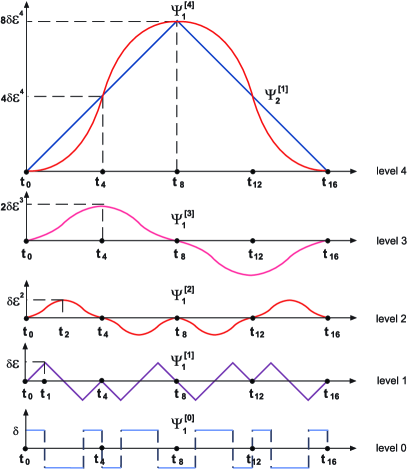
Figure 3: Hierarchical structure of geometrical patterns corresponding to the process. The isomorphism allows us to see a direct picture of the geometrical patterns, prime integer relations and correlations all together. For example, through the integration of the function $\Psi_{1}^{[l]},l=1,2,3$ we can see how the prime integer relations of level $l$ become the prime integer relations of the higher level. The functions $\Psi_{1}^{[1]},...,\Psi_{1}^{[4]}$ express the prime integer relations and can be used to measure the effect of correlations on the elementary parts. Remarkably, through the prime integer relations arithmetic defines how the boundary curves of the geometrical patterns must be curved. Notably, all geometrical patterns are symmetrical. Moreover, the symmetries are interconnected through the process and belong to one large symmetry of the hierarchical network.

Now, let us consider how the geometrical pattern can be characterized. In this regard, two characteristics of the geometrical pattern of the $j$th part $j=1,...,2^{k-l}$ at level $l=1,...,k$ are especially important.

First, it is the base $D_{jl}$, i.e., the length of the line segment with the endpoints at $(2^{l}(j-1)\varepsilon,0)$ and $(2^{l}j\varepsilon,0)$, and thus

$$D_{jl}=2^{l}\varepsilon.$$

Second, it is the height $H_{jl}$, i.e., the length of the line segment with one endpoint at the center $(2^{\frac{3}{2}l}j\varepsilon,0)$ of the geometrical pattern and the other at the point $(2^{\frac{3}{2}l}j\varepsilon,\Psi^{[l]}_{1}(2^{\frac{3}{2}l}j\varepsilon))$. The height $H_{jl}$ is equal to the extremum of the function $\Psi^{[l]}_{1}(t)$ on the interval

$$2^{l}(j-1)\varepsilon\leq t\leq 2^{l}j\varepsilon,$$

which is attained at the center of the geometrical pattern and hence

$$H_{jl}=|\Psi^{[l]}_{1}(2^{\frac{3}{2}l}j\varepsilon)|.$$

It turns out that Korotkikh_3

$$D_{l}=D_{jl},\ \ \ H_{l}=H_{jl},$$

$$j=1,...,2^{k-l},\ \ \ l=1,...,k.$$

Significantly, by using the base $D_{jl}$ and the height $H_{jl}$ alone we can find the area of the geometrical pattern. In fact, although the geometrical pattern of the $j$th part $j=1,...,2^{k-l}$ at level $l=2,...,k$ is not a triangle, yet, due to the condition (8), the boundary curve, as the graph of the function $\Psi^{[l]}_{1}$, provides a remarkable property: the area $A_{jl}$ of the geometrical pattern can be simply calculated by

$$A_{l}=A_{jl}=\frac{D_{l}H_{l}}{2}=\frac{D_{jl}H_{jl}}{2}.$$ (9)

As under the process the geometrical patterns of two parts at level $l=0,...,k-1$ transform into the geometrical pattern of the part at level $l+1$, the transformation connects the geometrical patterns and thus their characteristics with consequences for the parts at two different levels.

In particular, the base $D_{l}$ of the geometrical pattern of a part at level $l=1,...,k$ equals the sum

$$D_{l}=D_{l-1,left}+D_{l-1,right}=2D_{l-1}$$

of the bases of two geometrical patterns of the parts, while each geometrical pattern at level $l-1$ has the base

$$D_{l-1}=2^{l-1}\varepsilon.$$

By using the fundamental theorem of calculus we can find that the areas $A_{l-1}$ of the geometrical patterns of two parts at level $l-1$ equals the height $H_{l}$ of the geometrical pattern of the part they produce at level $l=1,...,k$

$$H_{l}=A_{l-1}.$$ (10)

From (9) and (10) we can obtain a recursive formula

$$H_{l}=A_{l-1}=\frac{D_{l-1}H_{l-1}}{2}$$

connecting the heights of the geometrical patterns of levels $l=1,...,k$ and $l-1$ and use it to express the area of the geometrical pattern of a part at level $l=0,...,k$ as

$$A_{l}=2^{\frac{l(l-1)}{2}}\varepsilon^{l+1}\delta.$$

Moreover, we can find the difference between the area of the geometrical pattern of a part at level $l=1,...,k$ and the sum of the areas of the geometrical patterns of the parts at level $l-1$ from which the part is made of

$$\Delta A_{l,l-1}=A_{l}-2A_{l-1}$$

$$=2^{\frac{l(l-1)}{2}}\varepsilon^{l+1}\delta-2\cdot 2^{\frac{(l-1)(l-2)}{2}}\varepsilon^{l}\delta$$

$$=2^{\frac{l(l-3)}{2}}\varepsilon^{l}\delta(2^{l}\varepsilon-2^{2}).$$

Since, according to (1), $\varepsilon\geq 1$, then the area of the geometrical pattern for all levels when $l\geq 2$ is greater than the sum of the areas of the geometrical patterns it is composed of

$$\Delta A_{l,l-1}=2^{\frac{l(l-3)}{2}}\varepsilon^{l}\delta(2^{l}\varepsilon-2^{2})>0,$$ (11)

except when $l=2,\ \varepsilon=1$, we get

$$\Delta A_{21}=2^{-1}\delta(2^{2}-2^{2})=0.$$

Notably, in the formation from level $0$ to level $1$ the difference between the areas is

$$\Delta A_{10}=\varepsilon^{2}\delta-2\varepsilon\delta=\varepsilon\delta(\varepsilon-2)$$ (12)

and, therefore, $\Delta A_{10}>0$ when $\varepsilon>2$, $\Delta A_{10}=0$ when $\varepsilon=2$, but $\Delta A_{10}<0$ when $\varepsilon<2$.

Consequently, for $l=1,\ \varepsilon\geq 2$ and $l\geq 2$ when two geometrical patterns combine, the area of the geometrical pattern they produce can only stay the same or increase, but can not decrease. However, for $l=1,\ \varepsilon<2$ the area indeed decreases.

Remarkably, a prime integer relation can be seen as a multifunctional entity. Two functions of the prime integer relation are especially important. They combine the characterization of an elementary part in the hierarchical network in terms of information and the characterization of the elementary part in space and time in terms of energy.

First, a prime integer relation can be seen as a storage as well as a carrier of information. Namely, a prime integer relation does contain information and in the realization of the correlations communicates the information to the elementary parts. Importantly, this function of the prime integer relation can be entirely expressed by the geometrical pattern, where the area of the geometrical pattern can be associated with the amount of information transmitted to the elementary parts and the area of the geometrical pattern of an elementary part can be associated with the amount of information received by the elementary part.

As a result, a part at level $l=1,...,k$ can be characterized by the information or the entropy $S_{l}$ of a corresponding prime integer relation and measured by the area $A_{l}$ of the geometrical pattern. Therefore, for the entropy $S_{l}$ of a part at level $l=1,...,k$ we obtain

$$S_{l}=A_{l}.$$ (13)

Second, a prime integer relation can be also seen as a source of energy. Namely, in the hierarchical network the law governing a part is actually the law of arithmetic given by a corresponding prime integer relation. Significantly, in the description the law of arithmetic can be fully expressed by the geometrical pattern and written in terms of the variables of its quantitative representation.

In particular, once the space and time coordinates of the elementary part are defined to encode the boundary curve and the area of the geometrical pattern is associated with the energy of the elementary part, the representation of the geometrical pattern become completed. Therefore, in the space and time representation the energy $E_{l}$ of a part at level $l=1,...,k$ can be defined by the sum of the energies of the elementary parts and thus to be equal to the area of the geometrical pattern

$$E_{l}=A_{l}.$$ (14)

Since through the geometrical pattern the motion of the elementary parts is fully determined by the prime integer relation, the prime integer relation can be seen as a source of energy making the motion of the elementary parts possible.

From (13) and (14), we obtain

$$S_{l}=E_{l}$$

and thus that the entropy of the part equals its energy. However, it should be mentioned that these two quantities characterize the part in two different arenas, i.e., the hierarchical network and space and time accordingly.

Notably, the condition (13) shows that the entropy of a prime integer relation is proportional to the surface area of the geometrical pattern. Therefore, the condition (13) reproduces the well-known connection between the entropy of a black hole and the area of its surface Bekenstein_1 ,Hawking_1 , but in its own terms.

Now, let us express the difference between the entropy of a part at level $l=1,...,k$ and the sum of the entropies of the parts at level $l-1$ the part is made of

$$\Delta S_{l,l-1}=S_{l}-2S_{l-1}=A_{l}-2A_{l-1}$$

$$=\Delta A_{l,l-1}=2^{\frac{l(l-3)}{2}}\varepsilon^{l}\delta(2^{l}\varepsilon-2^{2}).$$

As a result, from (11) and (12) we obtain that for $l=1,\ \varepsilon\geq 2$ and $l\geq 2$, when two parts combine, the entropy of the part they compose can only stay the same or increase, but can not decrease. More significantly, however, according to (12), we find that for $l=1,\ \varepsilon<2$ the entropy, in fact, decreases.

Therefore, the description might open a new way to explain the second law of thermodynamics Carno_1 -Boltzmann_1 . Moreover, by revealing the special case when the entropy decreases, the description raises the possibility that the second law of thermodynamics can loose its generality and appear as a manifestation of a more fundamental entity, i.e., the self-organization processes of prime integer relations and thus arithmetic.

Likewise, for the energy we get

$$\Delta E_{l,l-1}=E_{l}-2E_{l-1}=A_{l}-2A_{l-1}$$

$$=\Delta A_{l,l-1}=2^{\frac{l(l-3)}{2}}\varepsilon^{l}\delta(2^{l}\varepsilon-2^{2}).$$ (15)

Importantly, this means that under the process, except for $l=1,\ \varepsilon\leq 2$ and $l=2,\ \varepsilon=1$, the energy of a part is greater than the sum of the energies of the parts it is made of and thus with each next level the energy increases. However, the most striking finding from (15) is that the energy can be simply lost, when $l=1,\ \varepsilon<2$.

The following extremum principle can be formulated: for given $\varepsilon$ and $\delta$ in the formation of a part of a level from the parts of the lower level the energy of the part has to be extremized under the constraint of the prime integer relation.

Therefore, in the description arithmetic could be associated with a source of energy controlled through the processes with the consequences determined by the geometrical form. This source of energy may be already observed through dark energy and matter Riess_1 ,Perlmutter_1 , yet, it would be a completely different story to be able to use it for technological advances.

Moreover, arithmetic through a prime integer relation determines the distribution of the energy between the elementary parts and, consequently, produces a discrete energy spectrum. In this regard, it is important to note that a prime integer relation and thus its geometrical pattern are very sensitive and can not be changed. Indeed, even a minor change to the geometrical pattern results in the breaking of the relationships provided by the prime integer relation and thus the part falls apart. Therefore, the areas of the geometrical patterns of the elementary parts and their energies have to be absolutely fixed Korotkikh_6 -Korotkikh_9 .

For example, it can be found that the energy spectrum of the elementary parts $P_{14},...,P_{16,4}$ at level $4$ is a set of quantized values

$$E(P_{14}),...,E(P_{84})=$$

$$\frac{1}{120},\frac{29}{120},\frac{149}{120},\frac{361}{120},\frac{599}{120},\frac{811}{120},\frac{931}{120},\frac{959}{120},$$

where

$$E(P_{j4})=E(P_{17-j,4}),\ \ \ j=1,...,8$$

and $\varepsilon=1,\ \delta=1$. Clearly, the energy $E(P_{j4})$ of an elementary part $P_{j4},j=1,...,16$ can be given by the equation

$$E(P_{j4})=h_{4}\nu(P_{j4}),$$ (16)

where $h_{4}=\frac{1}{120}$ and $\nu(P_{j4})$ is an integer.

Similarly, the energy spectrum of the elementary parts $P_{15},...,P_{32,5}$ at level $5$ is a set of quantized values

$$E(P_{15}),...,E(P_{16,5})=$$

$$\frac{1}{720},\frac{61}{720},\frac{539}{120},\frac{2039}{720},\frac{4919}{720},\frac{9179}{720},\frac{14461}{720},\frac{20161}{720},$$

$$\frac{25919}{720},\frac{31619}{720},\frac{36901}{120},\frac{41161}{720},$$

$$\frac{44041}{720},\frac{45541}{720},\frac{46019}{720},\frac{46079}{720},$$

where

$$E(P_{j5})=E(P_{33-j,5}),\ \ \ j=1,...,16$$

and $\varepsilon=1,\ \delta=1$. In this case the energy $E(P_{j5})$ of an elementary part $P_{j5},j=1,...,32$ can given by the equation

$$E(P_{j5})=h_{5}\nu(P_{j5}),$$ (17)

where $h_{5}=\frac{1}{720}$ and $\nu(P_{j5})$ is an integer.

Interestingly, many of the integers in (16) and (17) are actually prime numbers. It seems like to make the elementary parts different, arithmetic tries to define their energies by using prime numbers. Note that (16) and (17) look similar to the Planck’s equation Planck_1 .

The two-dimensional character of the geometrical pattern suggests another important way to express the energy $E(P_{jl})$ of an elementary part $P_{jl},j=1,...,N,\ l=0,...,k$. In particular, let $C^{2}_{l}$ be a unit of two-dimensional area at level $l$, then, since the energy $E(P_{jl})$ of an elementary part $P_{jl}$ is given by the area of the geometrical pattern, we can write an equation

$$E(P_{jl})=M(P_{jl})C^{2}_{l},$$ (18)

which introduces the mass $M(P_{jl})$ of the elementary part. In symbolic appearance the equation looks similar to the Einstein’s formula Einstein_1 . Importantly, by using the equation (18) we can explain why the mass of the elementary part has the value that it does and not even slightly otherwise.

IV From a Scale Invariance to a Picture of the Hierarchical Network

In the hierarchical network of prime integer relations the process can progress through all levels and thus may be used to provide information about it as a whole. In fact, the following effective representation of the process allows us to obtain a first resolution picture of the hierarchical network.

The representation is based on a scale-invariant property of the process suggesting to arrange the levels into the groups of three successive levels. In particular, by using renormalizations in such a group the process can be given by a series of approximations, where the first term of the series characterizes the process in a self-similar way to the characterization at levels $1,2$ and $3$, and each next term reveals the process at a finer resolution. In other words, while the higher the level the process reaches to, the more complex it becomes with more terms in the series, yet the first term is always characterizes the process self-similarly to its characterization at levels $1,2$ and $3$.

More specifically, in the representation the levels are considered through the groups of three consecutive levels

$$\Pi_{1},...,\Pi_{p},\ \ \ p=1,2,...\ ,\ \ \ N=2^{3p+1}$$

and in a group $\Pi_{l},l=1,...,p$ of levels

$$3(l-1)+1,\ 3(l-1)+2,\ 3(l-1)+3$$

the process can be specified by a series of functions

$$\Psi^{[1]}_{l},\Psi^{[4]}_{l-1},...,\Psi^{[3(l-1)+1]}_{1},$$

where the function $\Psi^{[3(l-j)+1]}_{j},j=1,...,l$ encodes the formation of the parts at level $3(l-1)+1$ from the parts as basic elements at level $3(j-1)+1$. The representation demonstrates two important properties that are based on the condition (8).

First, the characterization of the process by using functions

$$\Psi^{[1]}_{l},\Psi^{[2]}_{l},\Psi^{[3]}_{l}$$

in a group $\Pi_{l},l=2,...,p$ of levels

$$3(l-1)+1,\ 3(l-1)+2,\ 3(l-1)+3$$

turns out to be self-similar to the characterization of the process by using functions

$$\Psi^{[1]}_{j},\Psi^{[2]}_{j},\Psi^{[3]}_{j}$$

in a group $\Pi_{j},j=1,...,l-1$ of levels

$$3(j-1)+1,\ 3(j-1)+2,\ 3(j-1)+3,$$

i.e., the characterization is the same except it is given in terms of $\varepsilon_{l}$ and $\delta_{l}$ rather than in terms of $\varepsilon_{j}$ and $\delta_{j}$, while the parameters are connected by the renormalizations

$$\varepsilon_{j+1}=2^{3}\varepsilon_{j},\ \delta_{j+1}=\varepsilon^{3}_{j}\delta_{j},\ j=1,...,l-1,$$

where $\varepsilon_{1}=\varepsilon,\ \delta_{1}=\delta$.

In the group $\Pi_{1}$ at level $1$ the process forms the parts

$${\cal P}_{11}^{\eta_{1}}=(P_{10}^{\eta_{1}}\leftrightarrow P_{20}^{\eta_{2}})^{\eta_{1}},...,$$

$${\cal P}_{N/2,1}^{\eta_{N/2}}=(P_{N-1,0}^{\eta_{N-1}}\leftrightarrow P_{N0}^{\eta_{N}})^{\eta_{N/2}},$$

where an elementary part $P_{j0}^{\eta_{j}},\ j=1,...,N$ at level $0$ can be positive if $\eta_{j}=1$ or negative if $\eta_{j}=-1$ and the symbol $\leftrightarrow$ means that the elementary parts are connected through a corresponding prime integer relation.

A part ${\cal P}_{j1}^{\eta_{j}},j=1,...,N/2$ is defined as a basic element, when the boundary curve of its geometrical pattern is given by the function (Figure 3)

$$\Psi^{[1]}_{1}(t+2(j-1)\varepsilon_{1})=\eta_{j}\Psi^{[1]}_{1}(t),\ \ \ 0\leq t\leq 2\varepsilon_{1},$$

where

$$\Psi^{[1]}_{1}(t)=\left\{\begin{array}[]{cl}\delta_{1}t,\ 0\leq t\leq\varepsilon_{1}\\ -t+2\varepsilon_{1},\ \varepsilon_{1}\leq t\leq 2\varepsilon_{1}.\end{array}\right.$$

In a group $\Pi_{l}$ at level $3(l-1)+1,\ l=2,...,p$ the parts

$${\cal P}_{1,3(l-1)+1}^{\eta_{1}},...,{\cal P}_{N/2^{3(l-1)+1},3(l-1)+1}^{\eta_{N/2^{3(l-1)+1}}}$$

formed by the process from the parts as basic elements at level $3(l-2)+1$ in their turn can be defined as basic elements at level $3(l-1)+1$, when the boundary curve of the geometrical pattern of a part

$${\cal P}_{j,3(l-1)+1}^{\eta_{j}},j=1,...,N/2^{3(l-1)+1}$$

become specified by the function

$$\Psi^{[1]}_{l}(t+2(j-1)\varepsilon_{l})=\eta_{j}\Psi^{[1]}_{l}(t),\ \ \ 0\leq t\leq 2\varepsilon_{l},$$

where

$$\Psi^{[1]}_{l}(t)=\left\{\begin{array}[]{cl}\delta_{l}t,\ 0\leq t\leq\varepsilon_{l}\\ -t+2\varepsilon_{l},\ \varepsilon_{l}\leq t\leq 2\varepsilon_{l}\end{array}\right.$$

and the part ${\cal P}_{j,3(l-1)+1}^{\eta_{j}}$ is positive if $\eta_{j}=1$ or negative if $\eta_{j}=-1$.

At this step in the construction of the representation the renormalization

$$\varepsilon_{l}=2^{3}\varepsilon_{l-1},\ \ \ \delta_{l}=\varepsilon^{3}_{l-1}\delta_{l-1}$$

introduces new length scales, while the parts, each made of $8$ basic elements of level $3(l-2)+1$, are coarse-grained and become basic elements of level $3(l-1)+1$.

Second, although in a group $\Pi_{l}$ the parts at level

$$3(l-1)+q,\ l=1,...,p,\ q=1,2,3$$

can be viewed differently as encoded by the functions

$$\Psi^{[q]}_{l},\Psi^{[3+q]}_{l-1},...,\Psi^{[3(l-1)+q]}_{1},$$

yet, because the functions define the geometrical patterns with the same area

$$\int_{t_{(j-1)2^{3(l-1)+q}}}^{t_{j2^{3(l-1)+q}}}\Psi^{[q]}_{l}(t)dt$$

$$=\int_{t_{(j-1)2^{3(l-1)+q}}}^{t_{j2^{3(l-1)+q}}}\Psi^{[3+q]}_{l-1}(t)dt=...$$

$$=\int_{t_{(j-1)2^{3(l-1)+q}}}^{t_{j2^{3(l-1)+q}}}\Psi^{[3(l-1)+q]}_{1}(t)dt,$$

$$j=1,...,2^{3p+1}/2^{3(l-1)+q}$$ (19)

as well as the base and height, the parts can be characterized in the same manner. However, the lengths of the boundary curves of the geometrical patterns are different.

Therefore, in the representation, irrespective of the basic elements the part is made of, the energy of the part is conserved.

For example, Figure 3 shows that in the group $\Pi_{2}$ at level $4$ the function $\Psi^{[1]}_{2}$ gives the first term of the series of approximations in the characterization of the process. The function $\Psi^{[4]}_{1}$ gives the second and the last term in the finer resolution, where the basic elements of level $4$ can be seen as the objects composed from the basic elements of level $1$. Notably, the geometrical patterns of the first and second terms of the series have the same area, base and height.

The characterization by the function $\Psi^{[1]}_{l},l=2,...,p$ is much simpler than those by the functions $\Psi^{[4]}_{l-1},...,\Psi^{[3(l-1)+1]}_{1}$. It assumes that the parts at level $3(l-1)+1$ are basic elements, i.e., have no internal structure, and does not take into account that they are actually composite objects. At the same time the simplest characterization can provide the same information about a number of quantities of the part and, in this regard, the energy stands out remarkably.

Therefore, in a group $\Pi_{l},l=2,...,p$ at level

$$3(l-1)+q,\ q=1,2,3$$

the first term $\Psi^{[q]}_{l}$ of the series can be used as long as it gives enough information about the part. Moreover, if needed, the approximation can be improved by taking into account the corrections from the neglected levels up to the function $\Psi^{[3(l-1)+q]}_{1}$ providing the information in terms of the basic elements at level $1$.

It is useful to consider the representation from the reverse perspective given by the functions

$$\varphi_{1}(\tau)=\frac{\Psi^{[1]}_{p}(t)}{\varepsilon_{p}\delta_{p}},\ \ \ \varphi_{2}(\tau)=\frac{\Psi^{[4]}_{p-1}(t)}{\varepsilon_{p}\delta_{p}},...,$$

$$\varphi_{p}(\tau)=\frac{\Psi^{[3(p-1)+1]}_{1}(t)}{\varepsilon_{p}\delta_{p}},$$

$$\tau=\frac{t}{\varepsilon_{p}},\ \ \ 0\leq\tau\leq 2,\ \ \ 0\leq t\leq 2\varepsilon_{p},\ \ \ p=1,2,...\ .$$

These functions are linearly ordered in the sense that

$$\varphi_{l+1}(\tau)<\varphi_{l}(\tau),\ \ \ 0<\tau<\frac{1}{2},\ \ \ \frac{3}{2}<\tau<2,$$

$$\varphi_{l+1}(\tau)>\varphi_{l}(\tau),\ \ \ \frac{1}{2}<\tau<\frac{3}{2},\ l=1,...,p-1$$

and, since

$$0\leq\varphi_{l}(\tau)\leq 1,\ \ \ l=1,...,p,\ \ \ 0\leq\tau\leq 2,$$

can be viewed in the context of a unit circle (Figure 4).

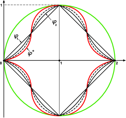
Figure 4: To help to understand how a unit circle could be defined in the hierarchical network the figure aims to represent the sequence of functions (21), but without taking into account the way they may intersect with the unit circle.

From the reverse perspective the conservation of the energy (19) takes the form

$$E=A=\int_{0}^{2}\varphi_{1}(\tau)d\tau=\int_{0}^{2}\varphi_{2}(\tau)d\tau\ =...$$

$$=\int_{0}^{2}\varphi_{l}(\tau)d\tau=1,$$ (20)

where $A$ is the area under each of the functions.

By comparing the perspectives we can note that, while the transition from the function $\Psi^{[4]}_{1}(t),\ 0\leq t\leq 2\varepsilon_{2}$ to the function $\Psi^{[1]}_{2}(t),\ 0\leq t\leq 2\varepsilon_{2}$ hides the information about the hierarchical structure of the part and thus makes it as a basic element, the transition from the function $\varphi_{1},\ 0\leq\tau\leq 2$ to the function $\varphi_{2},\ 0\leq\tau\leq 2$, however, reveals the hierarchical structure of the basic element. In particular, as the function $\varphi_{1}$ specifies the part as a basic element, the function $\varphi_{2}$ encodes the same part, but as a hierarchical structure made by the process from $8$ basic elements of level $1$.

In general, the sequence of functions

$$\varphi_{1},\varphi_{2},...,\varphi_{p},\ \ \ p=1,2,...$$ (21)

allows to consider the part at gradually smaller length scales. And while the function $\varphi_{1}$ specifies the part as a basic element, a function $\varphi_{l},\ l=2,...,p$ can reveal the part at a finer resolution, where it is built by the process from $2^{3l}$ basic elements. Moreover, the transition from a function $\varphi_{l},\ l=1,...,p-1$ to the function $\varphi_{l+1}$ reveals that the supposed to be basic elements are, in fact, divisible and have their own internal structure. Consequently, it turns out that the part is made by the process from $2^{3(l+1)}$ basic elements three more levels down.

However, it is interesting to know whether at least in the limit of the reductions

$$\lim_{p\to\infty}\varphi_{p}=\varphi^{*}$$ (22)

some basic elements not divisible any further can exist. In this regard, these reductions are quite remarkable. Indeed, although each next step probes the part at smaller length scales and its specification becomes more complex, yet, with each reduction the character of the basic elements remains the same thus suggesting that, in this sense, they are indivisible.

In the description a prime integer relation is a coherent system with rigid control of its components, but, at the same time, a very fragile one. As a prime integer relation is sensitive, so is the boundary curve of its geometrical pattern. This allows us to characterize the sequence of functions (21) by a fine-tuned parameter.

Namely, let $L_{l},\ l=1,...,p$ be the length of the boundary curve of the geometrical pattern defined by the graph of the function $\varphi_{l}$. The length $L_{l}$ of the boundary curve has an important property. In particular, because the exact value of $L_{l}$ corresponds to the prime integer relation, it becomes so sensitive that can not be changed even slightly. Whatever a small change of the value of $L_{l}$ can be, this will loose the correspondence with the prime integer relation. Therefore, the length $L_{l}$ has to be fine-tuned, unless its value is set exactly right, the relationships are not in place for the part to exist.

In view of this link and condition (20) a connection between the area of a geometrical pattern, as the energy of a corresponding part, and the length of the boundary curve may encode the distribution of the energy among the elementary parts. Now, let us specify such a connection.

In particular, by using functions $\varphi_{l}$ and $-\varphi_{l},\ l=1,...,p$ we can define a closed curve ${\mit\Gamma}_{l}$ and consider it in the context of the unit circle with the center at $(1,0)$ (Figure 4). The curves ${\mit\Gamma}_{1},...,{\mit\Gamma}_{p}$ in the limit of (22) can define a closed curve ${\mit\Gamma}^{*}$, which looks like a deformed circle.

By analogy with the ratio of a circle’s area $\pi r^{2}$ to its squared circumference $4\pi^{2}r^{2}$, a parameter $a_{l},l=1,...,p$ can be defined through the closed curve ${\mit\Gamma}_{l}$ to get a connection between the area of the geometrical pattern and the length of its boundary curve

$$2A=2\pi a_{l}(2L_{l})^{2},$$

where $2A$ is the area enclosed by the curve ${\mit\Gamma}_{l}$, $2L_{l}$ is the length of the curve and $2\pi$ is a normalization factor. Therefore, the parameter

$$a_{l}=\frac{2A_{l}}{2\pi(2L_{l})^{2}}=\frac{A}{4\pi L_{l}^{2}}$$

relates the area of the geometrical pattern and the length of the boundary curve, where $A_{l}=A=1$. Due to the character of $L_{l}$ the parameter $a_{l}$ is fine-tuned.

We can calculate

$$a_{1}=\frac{A_{1}}{2\pi L_{1}^{2}}=0.0099471839...\approx\frac{1}{101},$$

where $\varepsilon=1,\ \delta=1$ (Figure 4).

To find $a_{2}$ we can use the polynomial expressions of the function $\Psi^{[4]}_{1}(t),\ t_{0}\leq t\leq t_{16}$

$$\Psi_{1}^{[4]}(t)=\frac{t^{4}}{4!},\ \ \ t\in[t_{0},t_{1}],$$

$$\Psi_{1}^{[4]}(t)=-\frac{t^{4}}{4!}+\frac{t^{3}}{3}-\frac{t^{2}}{2}+\frac{t}{3}-\frac{1}{12},\ \ \ t\in[t_{1},t_{2}],$$

$$\Psi_{1}^{[4]}(t)=-\frac{t^{4}}{4!}+\frac{t^{3}}{3}-\frac{t^{2}}{2}+\frac{t}{3}-\frac{1}{12},\ \ \ t\in[t_{2},t_{3}],$$

$$\Psi_{1}^{[4]}(t)=\frac{t^{4}}{4!}-\frac{2t^{3}}{3}+4t^{2}-\frac{26t}{3}+\frac{20}{3},\ \ \ t\in[t_{3},t_{4}],$$

$$\Psi_{1}^{[4]}(t)=-\frac{t^{4}}{4!}+\frac{2t^{3}}{3}-4t^{2}+\frac{38t}{3}-\frac{44}{3},\ \ \ t\in[t_{4},t_{5}],$$

$$\Psi_{1}^{[4]}(t)=\frac{t^{4}}{4!}-t^{3}+\frac{17t^{2}}{2}-\frac{87t}{3}+\frac{449}{12},\ \ \ t\in[t_{5},t_{6}],$$

$$\Psi_{1}^{[4]}(t)=\frac{t^{4}}{4!}-t^{3}+\frac{17t^{2}}{2}-\frac{87t}{3}+\frac{449}{12},\ \ \ t\in[t_{6},t_{7}],$$

$$\Psi_{1}^{[4]}(t)=-\frac{t^{4}}{4!}+\frac{4t^{3}}{3}-16t^{2}+\frac{256t}{3}-\frac{488}{3},\ \ \ t\in[t_{7},t_{8}].$$

$$\Psi_{1}^{[4]}(t)=-\frac{t^{4}}{24}+\frac{4t^{3}}{3}-16t^{2}+\frac{256t}{3}-\frac{488}{3},\ \ \ t\in[t_{8},t_{9}],$$

$$\Psi_{1}^{[4]}(t)=\frac{t^{4}}{24}-\frac{5t^{3}}{3}+\frac{49t^{2}}{2}-\frac{473t}{3}+\frac{9218}{24},\ \ \ t\in[t_{9},t_{10}],$$

$$\Psi_{1}^{[4]}(t)=\frac{t^{4}}{24}-\frac{5t^{3}}{3}+\frac{49t^{2}}{2}-\frac{473t}{3}+\frac{9218}{24},\ \ \ t\in[t_{10},t_{11}],$$

$$\Psi_{1}^{[4]}(t)=-\frac{t^{4}}{24}+2t^{3}-36t^{2}+\frac{858t}{3}-836,\ \ \ t\in[t_{11},t_{12}],$$

$$\Psi_{1}^{[4]}(t)=\frac{t^{4}}{24}-2t^{3}+36t^{2}-290t+892,\ \ \ t\in[t_{12},t_{13}],$$

$$\Psi_{1}^{[4]}(t)=-\frac{t^{4}}{24}+\frac{7t^{3}}{3}-\frac{97t^{2}}{2}+\frac{1327t}{3}-\frac{35714}{24},\ \ \ t\in[t_{13},t_{14}],$$

$$\Psi_{1}^{[4]}(t)=-\frac{t^{4}}{24}+\frac{7t^{3}}{3}-\frac{97t^{2}}{2}+\frac{1327t}{3}-\frac{35714}{24},\ \ \ t\in[t_{14},t_{15}],$$

$$\Psi_{1}^{[4]}(t)=\frac{t^{4}}{24}-\frac{8t^{3}}{3}+64t^{2}$$

$$-\frac{2048t}{3}+\frac{8192}{3},\ \ \ t\in[t_{15},t_{16}]$$ (23)

to get $\varphi_{2}$ and then by computations obtain

$$a_{2}=\frac{A_{2}}{2\pi L_{2}^{2}}=0.0084640979...\approx\frac{1}{118},$$

where $\varepsilon=1,\ \delta=1$.

Although digits in the value of $a_{1}$ and $a_{2}$ seem to appear at random, yet, each digit there must stand as it is and not be even a bit different. Remarkably, our description can explain the values of the parameter, which are uniquely fixed and protected by arithmetic through the corresponding prime integer relations.

Since the function $\Psi_{1}^{[4]}$ belongs to level $4$, the four quantities $(\ref{SectionII.2})$ of the complex system remain unchanged. This invariance can be expressed by the conservation of four quantum numbers of the elementary parts as the first four coefficients of their polynomials.

In particular, from (23) we can find that the sum of the first quantum numbers

$$+\frac{1}{4!}-\frac{1}{4!}-\frac{1}{4!}+\frac{1}{4!}-\frac{1}{4!}+\frac{1}{4!}+\frac{1}{4!}-\frac{1}{4!}$$

$$-\frac{1}{4!}+\frac{1}{4!}+\frac{1}{4!}-\frac{1}{4!}+\frac{1}{4!}-\frac{1}{4!}-\frac{1}{4!}+\frac{1}{4!}=0,$$

the sum of the second quantum numbers

$$0+\frac{1}{3}+\frac{1}{3}-\frac{2}{3}+\frac{2}{3}-1-1+\frac{4}{3}+\frac{4}{3}$$

$$-\frac{5}{3}-\frac{5}{3}+2-2+\frac{7}{3}+\frac{7}{3}-\frac{8}{3}=0,$$

the sum of the third quantum numbers

$$0-\frac{1}{2}-\frac{1}{2}+4-4+\frac{17}{2}+\frac{17}{2}-16-16$$

$$+\frac{49}{2}+\frac{49}{2}-36+36-\frac{97}{2}-\frac{97}{2}+64=0$$

and the sum of the fourth quantum numbers

$$0+\frac{1}{3}+\frac{1}{3}-\frac{26}{3}+\frac{38}{3}-\frac{87}{3}-\frac{87}{3}+\frac{256}{3}+\frac{256}{3}-\frac{473}{3}$$

$$-\frac{473}{3}+\frac{858}{3}-290+\frac{1327}{3}+\frac{1327}{3}-\frac{2048}{3}=0.$$

Therefore, the quantum numbers are all preserved.

V Transformation of Laws of Arithmetic into Laws of Space and Time

In the previous section we have obtained a first resolution picture of the hierarchical network, where the correlation structure determined by the process at levels $1,2$ and $3$ is isomorphically represented by a hierarchical structure of two-dimensional geometrical patterns.

In this section we consider the transformation of the laws of arithmetic the elementary parts of the correlation structure are determined by in the hierarchical network into the laws of the elementary parts in space and time. Significantly, the laws of arithmetic can be fully expressed by the hierarchical structure of geometrical patterns and for an elementary part are entirely given by its geometrical pattern Korotkikh_1 -Korotkikh_6 .

The geometrical pattern of an elementary part has two defining entities, i.e., the boundary curve and the area. In the transformation we represent the boundary curve by the space and time coordinates of the elementary part and the area by the energy of the elementary part Korotkikh_6 -Korotkikh_9 .

Now, let us consider how the boundary curves of the elementary parts can be represented by using space and time as dynamical variables (Figure 3).

At level $0$ the space and time coordinates of an elementary part $P_{j0},j=1,...,16$ are defined through the arithmetical and geometrical forms of the description. In the arithmetical form at level $0$, where the integers have no relationships, nothing acts on the elementary part $P_{j0}$ and, therefore, it can be defined in the state of rest. In the geometrical form, the boundary curve of the elementary part $P_{j0}$ is given by the piecewise constant function

$$\Psi^{[0]}_{1}(t),\ t_{j-1}\leq t<t_{j}$$

and can be represented by the space and time coordinates of the elementary part $P_{j0}$ as follows. Namely, at the moment $T_{j0}(t_{j-1})=0$ of the local time, in the transition from one state into another, the space coordinate $X_{j0}(t_{j-1})$ of the elementary part $P_{j0}$ changes by

$$\Delta X_{j0}=\Psi^{[0]}_{1}(t_{j-1})=\eta_{j}\delta$$

and then stays as it is, while the time coordinate

$$T_{j0}(t),\ t_{j-1}\leq t<t_{j},$$

changes independently with the length of the boundary curve

$$\Delta T_{j0}(t)=T_{j0}(t)-T_{j0}(t_{j-1})=T_{j0}(t)$$

$$=\int_{t_{j-1}}^{t}\sqrt{1+(\frac{d\Psi^{[0]}_{1}}{dt})^{2}}dt,$$

where we set

$$\Delta T_{j0}=\lim_{t\to t_{j}}\int_{t_{j-1}}^{t}\sqrt{1+(\frac{d\Psi^{[0]}_{1}}{dt})^{2}}dt=\varepsilon.$$

Notably, no matter what the space coordinate is, the time coordinate is not affected.

Figure 3 shows that under the integration of the function $\Psi^{[l]}_{1}(t),\ l=0,1,2,\ t_{0}\leq t\leq t_{16}$ the geometrical patterns of the elementary parts at level $l$ transform into the geometrical patterns of the elementary parts at level $l+1$. As a result, the boundary curve of an elementary part $P_{jl},j=1,...,16$, i.e., the graph of the function

$$\Psi^{[l]}_{1}(t),\ t_{j-1}\leq t\leq t_{j},$$

transforms into the boundary curve of the elementary part $P_{j,l+1}$, i.e., the graph of the function

$$\Psi^{[l+1]}_{1}(t),\ t_{j-1}\leq t\leq t_{j}.$$

Significantly, under the transformations of the geometrical patterns space and time become dynamic variables defined by the representation of the boundary curves.

In particular, at level $1$ the space coordinate $X_{j1}(t)$ and time coordinate $T_{j1}(t),t_{j-1}\leq t\leq t_{j}$ of an elementary part $P_{j1},j=1,...,16$ become linearly dependent and characterize the motion of the elementary part $P_{j1}$ by

$$\Delta T_{j1}(t)sin(\alpha_{j})=\Delta X_{j1}(t),$$ (24)

with

$$\Delta X_{j1}(t)=X_{j1}(t)-X_{j1}(t_{j-1})$$

$$=\Psi^{[1]}_{1}(t)-\Psi^{[1]}_{1}(t_{j-1})$$ (25)

and

$$\Delta T_{j1}(t)=\int_{t_{j-1}}^{t}\sqrt{1+(\frac{d\Psi^{[1]}_{1}(t^{\prime})}{dt^{\prime}})^{2}}dt^{\prime}$$

$$=\int_{t_{j-1}}^{t}\sqrt{1+(\frac{dX_{j1}(t^{\prime})}{dt^{\prime}})^{2}}dt^{\prime},$$

where the angle $\alpha_{j}$ is given by

$$tan(\alpha_{j})=\Psi^{[0]}_{1}(t_{j-1}).$$

Let

$$\Delta X_{j1}=X_{j1}(t_{j})-X_{j1}(t_{j-1})$$

and, since $T_{j1}(t_{j-1})=0$,

$$\Delta T_{j1}=T_{j1}(t_{j})-T_{j1}(t_{j-1})=T_{j1}(t_{j}).$$

The velocity $V_{j1}(t),\ t_{j-1}\leq t\leq t_{j}$ of the elementary part $P_{j1}$, as a dimensionless quantity, can be defined by

$$V_{j1}(t)=\frac{\Delta X_{j1}(t)}{\Delta T_{j1}(t)}.$$ (26)

Applying conditions $(\ref{SectionV.1})$ and $(\ref{SectionV.3})$, we obtain

$$V_{j1}(t)=sin(\alpha_{j})$$

and, since the angle $\alpha_{j}$ is constant, the velocity is also a constant

$$V_{j1}(t)=V_{j1}.$$

By definition $-1\leq sin(a_{j})\leq 1$ and so

$$-1\leq V_{j1}\leq 1.$$ (27)

Since the velocity $V_{j1}$ is a dimensionless quantity, the condition $(\ref{SectionV.4})$ determines a velocity limit, which we associate with the speed of light $c$. We can now define the dimensional velocity $v_{j1}$ of the elementary part $P_{j1}$ by

$$V_{j1}=sin(\alpha_{j})=\frac{v_{j1}}{c}$$ (28)

and, therefore, $|v_{j1}|\leq c$.

By taking into account that at level $0$

$$|\Delta X_{j0}|=|\eta_{j}\delta|=|\pm\delta|=\delta,\ \ \ \Delta T_{j0}=\varepsilon,$$

from the geometry of the process at level $1$, we can find the dimensionless quantities

$$\frac{\chi_{j1}}{\chi_{min,j1}},\ \ \ \frac{\tau_{j1}}{\tau_{min,j1}}$$

of space and time of the elementary part $P_{j1}$.

In particular, for the dimensionless quantity

$$\frac{\chi_{j1}}{\chi_{min,j1}}$$

of space, by using $(\ref{SectionV.2})$, we obtain

$$\frac{\chi_{j1}}{\chi_{min,j1}}=|X_{j1}(t_{j})-X_{j1}(t_{j-1})|$$

$$=|\Psi^{[1]}_{1}(t_{j})-\Psi^{[1]}_{1}(t_{j-1})|=\delta\varepsilon=\frac{\chi_{0}}{\chi_{min}}\frac{\tau_{0}}{\tau_{min}}.$$ (29)

Therefore, the absolute change of the dimensional space coordinate of the elementary part $P_{j1}$ is $\chi_{0}\tau_{0}$. It sets the length scale of space at level $1$ as

$$\chi_{1}=\chi_{j1}=\chi_{0}\tau_{0},$$

while the minimum length scale of space $\chi_{min,1}$ at level $1$ is given by

$$\chi_{min,1}=\chi_{min,j1}=\chi_{min}\tau_{min}.$$

To find the dimensionless quantity

$$\frac{\tau_{j1}}{\tau_{min,j1}}$$

of time of the elementary part $P_{j1}$ we can use the Pythagorean theorem

$$\frac{\tau_{j1}^{2}}{\tau_{min,1}^{2}}=\varepsilon^{2}+\delta^{2}\varepsilon^{2}=\frac{\tau^{2}_{0}}{\tau_{min}^{2}}+\frac{\chi^{2}_{0}}{\chi_{min}^{2}}\frac{\tau^{2}_{0}}{\tau_{min}^{2}}$$

$$=\frac{\chi_{min}^{2}}{\chi_{min}^{2}}\frac{\tau^{2}_{0}}{\tau_{min}^{2}}+\frac{\chi^{2}_{0}}{\chi_{min}^{2}}\frac{\tau^{2}_{0}}{\tau_{min}^{2}}$$

and find

$$\frac{\tau_{j1}}{\tau_{min,1}}=\frac{\tau_{0}\sqrt{\chi_{min}^{2}+\chi^{2}_{0}}}{\chi_{min}\tau_{min}}.$$ (30)

According to $(\ref{SectionV.7})$, the change of the dimensional time coordinate of the elementary part $P_{j1}$ is

$$\tau_{1}=\tau_{j1}=\tau_{0}\sqrt{\chi_{min}^{2}+\chi^{2}_{0}}.$$

It sets the length scale of time at level $1$, while the minimum length scale of time at level $1$ is given by

$$\tau_{min,1}=\tau_{min,j1}=\chi_{min}\tau_{min}.$$

Importantly, by using conditions $(\ref{SectionV.6})$ and $(\ref{SectionV.7})$ we can express $\frac{v_{j1}}{c}$ as follows

$$|\frac{v_{j1}}{c}|=|sin(\alpha_{j})|=\frac{\frac{\chi_{0}}{\chi_{min}}\frac{\tau_{0}}{\tau_{min}}}{\frac{\tau_{0}\sqrt{\chi_{min}^{2}+\chi^{2}_{0}}}{\chi_{min}\tau_{min}}}=\frac{\chi_{0}}{\sqrt{\chi_{min}^{2}+\chi^{2}_{0}}}.$$ (31)

Therefore, the minimum length scale of space $\chi_{min}>0$ determines that the absolute value of the velocity $v_{j1}$ can not be equal to the velocity limit $c$. Indeed,

$$|\frac{v_{j1}}{c}|=\frac{\chi_{0}}{\sqrt{\chi_{min}^{2}+\chi^{2}_{0}}}<1$$

and thus

$$|v_{j1}|<c.$$

However, when $\chi_{min}=0$ or $\chi_{min}<<\chi_{0}$ the velocity $v_{j1}$ can become equal

$$|v_{j1}|=c$$ (32)

or very close to $c$.

The condition $(\ref{SectionV.9})$ suggests a parallel between the elementary parts of level $1$ and photons traveling at the speed of light. This actually motivated us to use the notation $c$ for the velocity limit and associate it with the speed of light.

Notably, when $\chi_{0}=\chi_{min}$, then

$$|\frac{v_{j1}}{c}|=\frac{\chi_{0}}{\sqrt{\chi_{min}^{2}+\chi^{2}_{0}}}$$

$$=\frac{\chi_{min}}{\sqrt{\chi_{min}^{2}+\chi_{min}^{2}}}=\frac{1}{\sqrt{2}}$$

and thus for the velocity $v_{j1}$ of the elementary part $P_{j1}$ we obtain

$$|v_{j1}|=\frac{c}{\sqrt{2}}.$$

As a result, we might say that when $\chi_{0}=\chi_{min}$ photons travel slower than in the case of $(\ref{SectionV.9})$.

Now, let us consider how the times $\Delta T_{j0}$ and $\Delta T_{j1}$ of the elementary parts $P_{j0}$ and $P_{j1},j=1,...,16$ can be connected. Note that, while there are no relationships to affect the elementary part $P_{j0}$ and thus it remains in the state of rest, the elementary part $P_{j1}$ is forced to move as a result of the relationship with another elementary part.

Figure 3 shows that

$$\Delta T_{j1}cos(\alpha_{j})=\Delta T_{j0}$$

and, by using $(\ref{SectionV.5})$, we get

$$\Delta T_{j1}=\frac{\Delta T_{j0}}{\sqrt{1-\frac{v_{j1}^{2}}{c^{2}}}}.$$ (33)

Since under the prime integer relations the correlations are realized simultaneously, then from $(\ref{SectionV.10})$ we can find that the time $T_{j1}(t)$ of the elementary part $P_{j1}$ runs faster than the time $T_{j0}(t),\ t_{j-1}\leq t\leq t_{j}$ of the elementary part $P_{j0}$.

Remarkably, the condition $(\ref{SectionV.10})$ symbolically reproduces the well-known formula connecting the elapsed times in the moving and the stationary systems Einstein_2 and allows its interpretation. In particular, as long as from a common perspective one tick of the clock of the moving elementary part $P_{j1}$ takes longer $\Delta T_{j1}>\Delta T_{j0}$ than one tick of the clock of the stationary elementary part $P_{j0}$, then the time counted by the number of ticks of the clock in the moving system will be less than the time counted by the number of ticks of the clock in the stationary system.

Notably, at level $1$ the motion of the elementary part $P_{j1}$ has the invariant

$$\Delta T_{j1}^{2}-\Delta X_{j1}^{2}=\varepsilon^{2}$$ (34)

with recognizable features of the Lorentz invariant.

Significantly, starting with level $2$, in the representation of the boundary curve the space and time coordinates of an elementary part $P_{jl},j=1,...,16,\ l=2,3$ become intimately linked, so that the boundary curve can be seen as their joint entity we define as the local spacetime of the elementary part $P_{jl}$. As for the boundary curves of the elementary parts at levels $0$ and $1$, we also define them as their local spacetimes.

In particular, in the representation of the boundary curve given by the graph of the function

$$\Psi^{[l]}_{1}(t),\ t_{j-1}\leq t\leq t_{j},\ j=1,...,16,\ l=2,3$$

the space coordinate $X_{jl}(t)$ of the elementary part $P_{jl}$ is defined by

$$X_{jl}(t)=\Psi^{[l]}_{1}(t),\ \ \ t_{j-1}\leq t\leq t_{j}.$$ (35)

In its turn the time coordinate $T_{jl}(t)$ of the elementary part $P_{jl}$ is defined by the length of the curve

$$T_{jl}(t)=\int_{t_{j-1}}^{t}\sqrt{1+(\frac{d\Psi^{[l]}_{1}(t^{\prime})}{dt^{\prime}})^{2}}dt^{\prime}$$

$$=\int_{t_{j-1}}^{t}\sqrt{1+(\frac{dX_{jl}(t^{\prime})}{dt^{\prime}})^{2}}dt^{\prime},\ \ \ t_{j-1}\leq t\leq t_{j}$$ (36)

and, as a result, the space and time coordinates become interdependent.

In the representation the motion of the elementary part $P_{jl}$ can be defined by the change of the space coordinate $X_{jl}(t)$ with respect to time coordinate $T_{jl}(t)$. Namely, as the time coordinate $T_{jl}(t)$ changes by

$$\Delta T_{jl}(t)=\int_{t_{j-1}}^{t}\sqrt{1+(\frac{d\Psi^{[l]}_{1}(t)}{dt})^{2}}dt$$

$$=\int_{t_{j-1}}^{t}\sqrt{1+(\frac{dX_{jl}(t)}{dt})^{2}}dt$$

the space coordinate $X_{jl}(t)$ changes by

$$\Delta X_{jl}(t)=\Psi^{[l]}_{1}(t)-\Psi^{[l]}_{1}(t_{j-1})$$

and we may say that under the correlations the position of the elementary part $P_{jl}$ during the time

$$\Delta T_{jl}=\int_{t_{j-1}}^{t_{j}}\sqrt{1+(\frac{d\Psi^{[l]}_{1}(t)}{dt})^{2}}dt$$

$$=\int_{t_{j-1}}^{t_{j}}\sqrt{1+(\frac{dX_{jl}(t)}{dt})^{2}}dt$$

changes by

$$\Delta X_{jl}=\Psi^{[l]}_{1}(t_{j})-\Psi^{[l]}_{1}(t_{j-1}).$$

For example, for the space coordinate $X_{12}(t)$ and time coordinate $T_{12}(t)$ of the elementary part $P_{12}$ we can get

$$X_{12}(t)=\frac{t^{2}}{2},\ \ \ t_{0}\leq t\leq t_{1}$$

and

$$T_{12}(t)=\int_{t_{0}}^{t}\sqrt{1+(\frac{dX_{12}(t^{\prime})}{dt^{\prime}})^{2}}dt^{\prime}$$

$$=\int_{t_{0}}^{t}\sqrt{1+t^{\prime 2}}dt^{\prime}$$

$$=\frac{t}{2}\sqrt{1+t^{2}}+\frac{1}{2}ln(t+\sqrt{1+t^{2}}),\ \ \ t_{0}\leq t\leq t_{1}.$$

We can obtain that

$$(\frac{dT_{12}(t)}{dt})^{2}-(\frac{dX_{12}(t)}{dt})^{2}=1.$$

Indeed,

$$\frac{dT_{12}(t)}{dt}=\frac{d}{dt}(\frac{t}{2}\sqrt{1+t^{2}}+\frac{1}{2}ln(t+\sqrt{1+t^{2}}))$$

$$=\frac{\sqrt{1+t^{2}}}{2}+\frac{t^{2}}{2\sqrt{1+t^{2}}}+\frac{1+\frac{t}{\sqrt{1+t^{2}}}}{2(t+\sqrt{1+t^{2}})}$$

$$=\frac{1+t^{2}+t^{2}}{2\sqrt{1+t^{2}}}+\frac{\sqrt{1+t^{2}}+t}{2(\sqrt{1+t^{2}})(t+\sqrt{1+t^{2}})}$$

$$=\sqrt{1+t^{2}}$$

and

$$\frac{dX_{12}(t)}{dt}=t,$$

so

$$(\frac{dT_{12}(t)}{dt})^{2}-(\frac{dX_{12}(t)}{dt})^{2}=1+t^{2}-t^{2}=1.$$

In general, by using $(\ref{SectionV.13})$, we can find that the motion of an elementary part $P_{jl},j=1,...,16,\ l=2,3$ has the following invariant

$$(\frac{dT_{jl}(t)}{dt})^{2}-(\frac{dX_{jl}(t)}{dt})^{2}=1$$ (37)

with the invariant $(\ref{SectionV.11})$ as a special case.

Notably, similar to level $1$, at levels $2$ and $3$ we can get linear approximations to the dynamics of the elementary parts that provide a Lorentz type invariant

$$\Delta\breve{T}_{jl}^{2}-\Delta\breve{X}_{jl}^{2}=\varepsilon^{2},$$ (38)

while preserving the sum of the energies of the elementary parts.

For example, at level $3$ the approximation for the part ${\cal P}_{13}^{+}$ is given by the functions

$$y=\frac{2\delta\varepsilon^{3}}{t_{4}}t,\ \ \ t_{0}\leq t\leq t_{4},$$

$$y=-\frac{2\delta\varepsilon^{3}}{t_{8}-t_{4}}t+\frac{2\delta\varepsilon^{3}}{t_{8}-t_{4}}t_{8},\ \ \ t_{4}\leq t\leq t_{8}$$

and at level $4$ the approximation for the part ${\cal P}_{14}^{+}$ is specified by the function $\Psi^{[1]}_{2}(t),\ t_{0}\leq t\leq t_{16}$ (Figure 3).

Next, we consider the connection between the local spacetime and the energy of an elementary part $P_{jl},j=1,...,16,\ l=0,1,2,3$ determined by the representation of the geometrical pattern. In particular, we can see that the boundary curve, i.e., the graph of the function $\Psi^{[l]}_{1}(t),\ t_{j-1}\leq t\leq t_{j}$, not only encodes the local spacetime, but also determines the energy of the elementary part $P_{jl}$

$$E_{jl}=\int_{t_{j-1}}^{t_{j}}|\Psi^{[l]}_{1}(t)|dt.$$

We can also define the energy density ${\cal E}_{jl}(t)$ of the elementary part $P_{jl}$

$$E_{jl}=\int_{t_{j-1}}^{t_{j}}{\cal E}_{jl}(t)dt=\int_{t_{j-1}}^{t_{j}}|\Psi^{[l]}_{1}(t)|dt$$

and, since (35), obtain

$${\cal E}_{jl}(t)=|X_{jl}(t)|,\ \ \ t_{j-1}\leq t\leq t_{j}$$ (39)

meaning that the energy density of the elementary part equals its space coordinate.

To consider the connection between the local spacetimes and the energies of elementary parts at different levels the energy profile $E_{jl}(t)$ of an elementary part $P_{jl},j=1,...,16,\ l=0,1,2$

$$E_{jl}(t)=\int_{t_{j-1}}^{t}|\Psi^{[l]}_{1}(t^{\prime})|dt^{\prime},\ \ \ t_{j-1}\leq t\leq t_{j}$$

can be useful. Indeed, by using the fundamental theorem of calculus we can find that the energy profile of the elementary part $P_{jl}$ at level $l$ determines the local spacetime of the elementary part $P_{j,l+1}$ at level $l+1$

$$X_{j,l+1}(t)=\Psi^{[l+1]}_{1}(t)=\int_{t_{0}}^{t}\Psi^{[l]}_{1}(t^{\prime})dt^{\prime}$$

$$=\int_{t_{0}}^{t_{j-1}}\Psi^{[l]}_{1}(t^{\prime})dt^{\prime}+\int_{t_{j-1}}^{t}\Psi^{[l]}_{1}(t^{\prime})dt^{\prime}$$

$$=X_{j,l+1}(t_{j-1})\pm E_{jl}(t),\ \ \ t_{j-1}\leq t\leq t_{j}.$$

In particular, when $t=t_{j}$, we get

$$|X_{j,l+1}(t_{j})-X_{j,l+1}(t_{j-1})|=E_{jl}$$

and, therefore, the energy of the elementary part $P_{jl}$ at level $l$ is equal to the change of the space coordinate of the elementary part $P_{j,l+1}$ at level $l+1$.

As the laws of the elementary parts in terms of arithmetic have been transformed into the laws of the elementary parts in terms of space and time, now let us consider the resulting structure of the local spacetimes.

Remarkably, Figure 3 shows the local spacetimes of the elementary parts all at once and helps to illustrate the notion of simultaneity in terms of the local spacetimes. Namely, as the correlation structure turns to be operational, then through the prime integer relations the elementary parts, irrespective of the distances and levels, all become instantaneously connected and move simultaneously, so that the local spacetimes can geometrically reproduce the prime integer relations in control of the correlation structure. In other words, the local spacetimes all function together to be mutually self-consistent in reproducing of the prime integer relations.

The local spacetime changes with the level and takes the shape precisely as determined by the prime integer relation. In particular, this defines that the time runs differently at the levels and we may say that the rate at which the clock ticks varies with the level of the correlation structure. Furthermore, for elementary parts of the same level the elapsed times can be also different. For example, it can be calculated that the space coordinate of the elementary part $P_{13}$ changes by $\Delta X_{13}=1/6$ during the time $\Delta T_{13}\approx 1.02$, while the space coordinate of the elementary part $P_{23}$ changes by $\Delta X_{23}=5/6$ during the time $\Delta T_{23}\approx 1.30$, when $\delta=1,\ \varepsilon=1$.

We may visualize the correlations at work by imagining some points that move along the boundary curves with simultaneous start and finish. Since the length of the trajectory of the point so far shows the time of the elementary part, then observing the point moving at level $l=2,3$ might seem like observing the time curving in the flow.

Notably, when the boundary curve is viewed as the geodesic of the elementary part, it appears that the elementary part moves from one point to another not to extremize an action in between, but to geometrically reproduce the prime integer relation. In other words, the prime integer relation guides the motion of the elementary part. Significantly, the geodesics of the elementary parts are elements of one and the same structure, i.e, the hierarchical network of prime integer relations.

In analogy with general relativity, where spacetime curves in respond to energy Einstein_3 , in our description the local spacetime of an elementary part also curves in accordance with the energy of the elementary part. Importantly, the dependence between the local spacetime and the energy appears as a result of the transformation of a corresponding law of arithmetic. Furthermore, the condition for an elementary part to be integrated into the correlation structure is entirely determined by the geometry of the local spacetime. Therefore, once we interpret that the elementary parts are held in the correlation structure by a force, then the force acting on an elementary part can be fully defined by the geometry of the local spacetime.

In general, Figure 3 gives us a powerful perspective. First, we can observe how the local spacetimes appear to be related to one another. Moreover, we can know in advance what will happen to the elementary parts even before the correlation structure become triggered. When that happens, the elementary parts are controlled nonlocally, but act locally for one common purpose to preserve the system. Second, the picture is timeless in the sense that past, present and future are all united in one whole still. Third, because the elementary parts move in their own local spacetimes, then by changing the focus from one elementary part to another seems like we travel not only in space, but in time as well.

VI Global Spacetimes as Effective Representations of the Hierarchical Network

In the previous section we have considered a representation of the hierarchical structure of geometrical patterns by using space and time as dynamic variables. As a result, the elementary parts become specified not in one global spacetime, where the laws of arithmetic they realize can be expressed by using the same number of space and time variables, but by local spacetimes and energies.

This fact is not surprising. As the process takes place not in space and time, but in the hierarchical network, rather than to emerge in a global spacetime, the local spacetimes have to make the geometrical patterns corresponding to the hierarchical structure of prime integer relations.

Remarkably, in the representation the elementary parts act as the carriers of the laws of arithmetic the process is governed by with each elementary part carrying its own quantum of the laws entirely determined by the geometrical pattern. This opens an important perspective to use elementary parts in the hierarchical network as quanta to construct different laws. In this regard, a global spacetime could serve as a common stage, where elementary parts would be combined with their quanta of the laws taking the form in terms of the same number of space and time variables. Significantly, once through the form of the laws a desired objective would be realized, the global spacetime could be used as an effective representation of the process.

In general, this perspective suggests the hierarchical network as a source of laws that could be harnessed. In particular, for a given objective the hierarchical network could be used to generate self-organization processes to obtain relevant laws of arithmetic and then process them into the required form by constructing a corresponding global spacetime.

In fact, the perspective allows us to speculate about an observing system that in the processing of the hierarchical network could be adaptable to obtain different effective representations. Furthermore, the description can provide a formal means in the context of the mind-matter problem Kant_1 -Penrose_1 to consider why the mind in the processing of the hierarchical network might be programmed to sense three dimensions of space and one dimension of time.

Significantly, an effective representation can not function, unless supported by an equivalence class of inertial reference frames, where the form of the laws is actually represented and thus the same. This determines a symmetry group of coordinate transformations with the form as the invariant and resonates well with the principle of relativity.

Historically, it has been established that physical laws can express themselves through the same form when considered in their inertial reference frames and this has resulted in the principle of relativity Einstein_2 . For example, in classical mechanics the Galilean transformations specify the inertial coordinate systems, while in electromagnetic theory the Lorentz transformations take responsibility for the transitions between the inertial reference frames.

However, the principle of relativity and the description may follow opposite directions. Namely, the principle of relativity, based on the success with a number of physical laws, is tried to make a leap forward and accommodate all physical laws. Clearly, it would be an ideal situation, instead of discovering laws one by one, to establish and maintain them all as one source of the physical laws to rely on when needed. For example, when a problem arises the source could be used to generate specific laws to solve the problem.

In the description, by contrast, all its possible laws are already given. They are the laws of arithmetic realized by the processes in the construction of the hierarchical network. Consequently, the hierarchical network appears as a source of laws that could be used to supply particular laws on demand by defining a corresponding global spacetime.

In this section we consider a number of effective representations of the process in terms of global spacetimes.

First, we consider a representation, where through the local spacetimes the elementary parts $P_{j1},P_{j2}$ and $P_{j3},j=1,...,16$ are combined by a global spacetime

$${\cal R}_{j}(3,3)={\cal R}_{j1}\times{\cal R}_{j2}\times{\cal R}_{j3}$$

as the direct product of two-dimensional Euclidean spaces ${\cal R}_{j1},{\cal R}_{j2}$ and ${\cal R}_{j3}$.

In particular, by using ${\cal R}_{jl},j=1,...16,\ l=1,2,3$ the space and time coordinates of the elementary part $P_{jl}$ are specified by a vector function

$${\bf R}_{jl}(t)=T_{jl}(t){\bf w}_{jl}+\sqrt{-1}X_{jl}(t){\bf u}_{jl}$$

$$=\sqrt{-1}X_{jl}(t){\bf u}_{jl}+T_{jl}(t){\bf w}_{jl},\ \ \ t_{j-1}\leq t\leq t_{j},$$ (40)

where ${\bf w}_{jl}$ and ${\bf u}_{jl}$ are the unit vectors of an orthogonal basis and, to preserve the invariant $(\ref{SectionV.15})$, the space coordinate is treated imaginary $\sqrt{-1}X_{jl}(t)$ with

$$(\sqrt{-1})^{2}=-1.$$

As a result, ${\cal R}_{jl}$ acquires a Minkowski spacetime type of signature $(-,+)$.

In the global spacetime ${\cal R}_{j}(3,3)$ the vector functions

$${\bf R}_{j1}(t),\ {\bf R}_{j2}(t),\ {\bf R}_{j3}(t),\ \ \ t_{j-1}\leq t\leq t_{j}$$

define the curves as the trajectories of the elementary parts $P_{j1},P_{j2}$ and $P_{j3}$. In particular, the curve given by the vector function ${\bf R}_{jl}(t),l=1,2,3$ can encode the space coordinate $X_{jl}(t)$ as a function of the time coordinate $T_{jl}(t)$ and thus the dynamics of the elementary part $P_{jl}$ in ${\cal R}_{j}(3,3)$.

Defined by the direct product of ${\cal R}_{j1},{\cal R}_{j2}$ and ${\cal R}_{j3}$ the six-dimensional global spacetime ${\cal R}_{j}(3,3)$ of three space and three time variables does not contain information about the formation and connection between the elementary parts $P_{j1},P_{j2}$ and $P_{j3}$. As a result, in the global spacetime the elementary parts become seen as separate entities.

Namely, the elementary part $P_{j1}$ is characterized by the vector function

$${\bf R}_{j1}(t)=\sqrt{-1}X_{j1}(t){\bf u}_{j1}+T_{j1}(t){\bf w}_{j1}$$

$$+\sqrt{-1}\cdot 0{\bf u}_{j2}+0{\bf w}_{j2}+\sqrt{-1}\cdot 0{\bf u}_{j3}+0{\bf w}_{j3}$$

$$=\sqrt{-1}X_{j1}(t){\bf u}_{j1}+\sqrt{-1}\cdot 0{\bf u}_{j2}+\sqrt{-1}\cdot 0{\bf u}_{j3}$$

$$+T_{j1}(t){\bf w}_{j1}+0{\bf w}_{j2}+0{\bf w}_{j3},\ \ \ t_{j-1}\leq t\leq t_{j}$$ (41)

with the space coordinates

$$\sqrt{-1}X_{j1}(t),\sqrt{-1}\cdot 0,\sqrt{-1}\cdot 0$$

and time coordinates

$$T_{j1}(t),0,0.$$

The elementary part $P_{j2}$ is characterized by the vector function

$${\bf R}_{j2}(t)=\sqrt{-1}\cdot 0{\bf u}_{j1}+0{\bf w}_{j1}$$

$$+\sqrt{-1}X_{j2}(t){\bf u}_{j2}+T_{j2}(t){\bf w}_{j2}$$

$$+\sqrt{-1}\cdot 0{\bf u}_{j3}+0{\bf w}_{j3}$$

$$=\sqrt{-1}\cdot 0{\bf u}_{j1}+\sqrt{-1}X_{j2}(t){\bf u}_{j2}+\sqrt{-1}\cdot 0{\bf u}_{j3}$$

$$+0{\bf w}_{j1}+T_{j1}(t){\bf w}_{j2}+0{\bf w}_{j3},\ \ \ t_{j-1}\leq t\leq t_{j}$$ (42)

with the space coordinates

$$\sqrt{-1}\cdot 0,\sqrt{-1}X_{j2}(t),\sqrt{-1}\cdot 0$$

and time coordinates

$$0,T_{j1}(t),0.$$

And, finally, the elementary part $P_{j3}$ is characterized by the vector function

$${\bf R}_{j3}(t)=\sqrt{-1}\cdot 0{\bf u}_{j1}+0{\bf w}_{j1}+\sqrt{-1}\cdot 0{\bf u}_{j2}+0{\bf w}_{j3}$$

$$+\sqrt{-1}X_{j3}(t){\bf u}_{j3}+T_{j3}(t){\bf w}_{j3}$$

$$=\sqrt{-1}\cdot 0{\bf u}_{j1}+\sqrt{-1}\cdot 0{\bf u}_{j2}+\sqrt{-1}X_{j3}(t){\bf u}_{j3}$$

$$+0{\bf w}_{j1}+0{\bf w}_{j2}+T_{j1}(t){\bf w}_{j3},\ \ \ t_{j-1}\leq t\leq t_{j}$$ (43)

with the space coordinates

$$\sqrt{-1}\cdot 0,\sqrt{-1}\cdot 0,\sqrt{-1}X_{j3}(t)$$

and time coordinates

$$0,0,T_{j1}(t).$$

By construction this reference frame is special and from $(\ref{SectionVI.2})$-$(\ref{SectionVI.4})$ we can clearly see that there exist preferred directions in the global spacetime ${\cal R}_{j}(3,3)$ thus making it anisotropic. However, the anisotropy might be hidden in a reference frame, where for the laws to have the same form the space and time coordinates of an elementary part $P_{jl},j=1,...,16,\ l=1,2,3$ would be transformed into the space coordinates

$$\sqrt{-1}X_{jl1}^{\prime}(t),\sqrt{-1}X_{jl2}^{\prime}(t),\sqrt{-1}X_{jl3}^{\prime}(t)$$

and time coordinates

$$T_{jl1}^{\prime}(t),T_{jl2}^{\prime}(t),T_{jl3}^{\prime}(t),$$

but preserving the invariant $(\ref{SectionV.15})$

$$(\frac{dT_{jl1}^{\prime}(t)}{dt})^{2}+(\frac{dT_{jl2}^{\prime}(t)}{dt})^{2}+(\frac{dT_{jl3}^{\prime}(t)}{dt})^{2}$$

$$-(\frac{dX_{jl1}^{\prime}(t)}{dt})^{2}-(\frac{dX_{jl2}^{\prime}(t)}{dt})^{2}-(\frac{dX_{jl3}^{\prime}(t)}{dt})^{2}$$

$$=(\frac{dT_{jl}(t)}{dt})^{2}-(\frac{dX_{jl}(t)}{dt})^{2}=1,\ \ \ t_{j-1}\leq t\leq t_{j}.$$ (44)

As a result, the elementary part $P_{jl}$ would be characterized by a vector function

$${\bf R}_{jl}^{\prime}(t)$$

$$=\sqrt{-1}X_{jl1}^{\prime}(t){\bf u}_{j1}^{\prime}+\sqrt{-1}X_{jl2}^{\prime}(t){\bf u}_{j2}^{\prime}+\sqrt{-1}X_{jl3}^{\prime}(t){\bf u}_{j3}^{\prime}$$

$$+\ T_{jl1}^{\prime}(t){\bf w}_{j1}^{\prime}+T_{jl2}^{\prime}(t){\bf w}_{j2}^{\prime}+T_{jl3}^{\prime}(t){\bf w}_{j3}^{\prime},$$ (45)

where $t_{j-1}\leq t\leq t_{j}$. Therefore, the invariant $(\ref{SectionVI.5})$ would define an equivalence class of inertial reference frames as well as a symmetry group of coordinate transformations.

By contrast with $(\ref{SectionVI.2})$-$(\ref{SectionVI.4})$, from $(\ref{SectionVI.6})$ the anisotropy of the global spacetime ${\cal R}_{j}(3,3)$ could not be explicitly seen. In fact, according to $(\ref{SectionVI.6})$ alone the elementary part $P_{jl}$ would be given in the global spacetime ${\cal R}_{j}(3,3)$ with the signature $(-,-,-,+,+,+)$ and characterized by three space coordinates and three time coordinates.

Obviously, it is unusual through the ordinary senses to experience three dimensions of time. Yet, as far as the description is concerned, three time coordinates as well as three space coordinates are determined by three levels of the hierarchical structure. Moreover, the three dimensions of time and thus the possibility to travel in time is a result of the fact that in the observation of the hierarchical structure it is possible not only to consider the local spacetime of any elementary part, but also change the focus from one elementary part to another and thus travel in time.

Notably, unlike the hierarchical structure, the representation does not tell the formation story. It simply does not have information about the formation, order and connections between the elementary parts. Yet, the representation could be effective as long as through the form of the laws the process would be harnessed by understanding the elementary parts in terms of the same space and time variables.

To recognize features of familiar global spacetimes let us first consider a representation of the process in terms of a four-dimensional global spacetime.

The representation can be obtained as a special case of ${\cal R}_{j}(3,3),j=1,...,16$, where the time coordinates of the elementary parts $P_{j1},P_{j2}$ and $P_{j3}$ are processed by using the same time variable. Specifically, in this case a two-dimensional Euclidean space ${\cal R}_{jl},j=1,...,16,\ l=1,2,3$ with an orthogonal basis of unit vectors ${\bf u}_{jl}$ and ${\bf w}_{j}$ is used to represent the space and time coordinates of the elementary part $P_{jl}$ by a vector function

$${\bf R}_{jl}(t)=\sqrt{-1}X_{jl}(t){\bf u}_{jl}+T_{jl}(t){\bf w}_{j},\ \ \ t_{j-1}\leq t\leq t_{j}.$$ (46)

We can see that in comparison with $(\ref{SectionVI.1})$ in $(\ref{SectionVI.7})$ the unit vector ${\bf w}_{j}$ for the time coordinate does not depend on the level of the elementary part and is the same for the Euclidean spaces ${\cal R}_{j1},{\cal R}_{j2}$ and ${\cal R}_{j3}$.

The direct product

$${\cal R}_{j}(3,1)={\cal R}_{j1}\times{\cal R}_{j2}\times{\cal R}_{j3}$$

gives a common stage to the elementary parts $P_{j1},P_{j2}$ and $P_{j3}$ and, similar to ${\cal R}_{j}(3,3)$, could be an effective representation of the process in terms of a four-dimensional global spacetime with the signature $(-,-,-,+)$, where the elementary parts $P_{j1},P_{j2}$ and $P_{j3}$ are characterized by three space coordinates and one time coordinate.

In particular, in this case the invariant $(\ref{SectionVI.5})$ takes the form

$$(\frac{dT_{jl}^{\prime}(t)}{dt})^{2}-(\frac{dX_{jl1}^{\prime}(t)}{dt})^{2}-(\frac{dX_{jl2}^{\prime}(t)}{dt})^{2}-(\frac{dX_{jl3}^{\prime}(t)}{dt})^{2}$$

$$=(\frac{dT_{jl}(t)}{dt})^{2}-(\frac{dX_{jl}(t)}{dt})^{2}=1,\ \ \ t_{j-1}\leq t\leq t_{j}$$ (47)

and the representation exists as long as it is supported by an equivalence class of inertial reference frames with the coordinate transformations preserving the invariant $(\ref{SectionVI.8})$, where $X_{jl1}^{\prime}(t),X_{jl2}^{\prime}(t),X_{jl3}^{\prime}(t)$ are the space coordinates and $T_{jl}^{\prime}(t)$ is the time coordinate of the elementary part $P_{jl}$ in such a frame of reference.

The character of the expression $(\ref{SectionVI.8})$ suggests to consider possible connections of the global spacetime ${\cal R}_{j}(3,1)$ with general relativity. In particular, while in general relativity tangent spaces have Minkowskian geometry, in the representation, by using linear approximations $(\ref{SectionV.16})$ preserving the sum of the energies of the elementary parts, we can write the invariant $(\ref{SectionVI.8})$ as

$$\Delta\breve{T}_{jl}^{\prime 2}-\Delta\breve{X}_{jl1}^{\prime 2}-\Delta\breve{X}_{jl2}^{\prime 2}-\Delta\breve{X}_{jl3}^{\prime 2}$$

$$=\Delta\breve{T}_{jl}^{2}-\Delta\breve{X}_{jl}^{2}=\varepsilon^{2}$$

and recognize familiar features of the Lorentz transformations in four-dimensional Minkowski space of special relativity.

Now, let us discuss possible connections of the invariants $(\ref{SectionVI.5})$ and $(\ref{SectionVI.8})$ with Lie groups. This might allow, in view of the developments initiated in Yang_1 , to consider $(\ref{SectionVI.5})$ in terms of a Yang-Mills gauge field and its equations, and, since general relativity is, in fact, the gauge field theory associated with the symmetry group of Lorentz transformations in Minkowski space Utiyama_1 , to derive the Einstein’s equations in the case of $(\ref{SectionVI.8})$.

It is well known that in terms of gauge fields the gravitational interaction is different from the electromagnetic, strong and weak interactions Utiyama_1 , Yang_2 . In this context it is interesting to consider whether the description can reveal a parallel.

In the description the interactions are realized through the prime integer relations. In particular, it can be interpreted that the elementary parts are held together in a part by interacting through the prime integer relation. Furthermore, to see the situation more traditionally a prime integer relation might be associated with a gauge field based on the symmetry group of the geometrical pattern.

In particular, let

$$f_{P_{jl}}={\cal A}_{jl1}t^{l}+...+{\cal A}_{jl,l+1}=\Psi^{[l]}_{1}(t),\ \ \ t_{j-1}\leq t\leq t_{j},$$

where ${\cal A}_{jl1},...,{\cal A}_{jll},j=1,...,16,\ l=1,2,3$ are the quantum numbers of the elementary part $P_{jl}$. To define the gauge field between the elementary parts $P_{jl}$ and $P_{j+1,l}$ of a part we consider the condition

$$f_{P_{jl}}+f_{{\bf P}_{j,j+1,l}}=f_{P_{j+1,l}}.$$ (48)

Since the difference

$$f_{P_{jl}}-f_{P_{j+1,l}}$$

$$=({\cal A}_{jl1}-{\cal A}_{j+1,l1})t^{l}+...+({\cal A}_{jl,l+1}-{\cal A}_{j+1,l,l+1})$$

is a polynomial itself

$$f_{{\bf P}_{j,j+1,l}}={\cal B}_{j,j+1,l,1}t^{l}+...+{\cal B}_{j,j+1,l,l+1},$$

where

$${\cal B}_{j,j+1,li}={\cal A}_{jli}-{\cal A}_{j+1,li},\ \ \ i=1,...,l+1$$

the gauge field between the elementary parts $P_{jl}$ and $P_{j+1,l}$ can be associated with an elementary part ${\bf P}_{j,j+1,l}$, but of a different type.

To be specific, by contrast with the elementary parts $P_{jl}$ and $P_{j+1,l}$, which experience the gauge field, the elementary part ${\bf P}_{j,j+1,l}$ communicates the field. We may view the field between the elementary parts $P_{jl}$ and $P_{j+1,l}$ as the exchange of the elementary part ${\bf P}_{j,j+1,l}$ and say that the gauge field is required, when the global symmetry of the geometrical pattern is converted into the local symmetry $(\ref{SectionVI.9})$.

Thus, in the description we can identify two types of elementary parts with two different roles. First, there are the elementary parts that experience fields and second, there are the elementary parts that communicate the fields. Remarkably, as equation $(\ref{SectionVI.9})$ shows, all elementary parts, in spite of their differences, are naturally united. It is also important to note that through three levels of the hierarchical structure we have three different symmetry groups, which are connected by the self-organization process.

Importantly, in identifying a gauge field, corresponding to the gravitational interaction, we might associate it with the symmetry based on the conservation of the invariant $(\ref{SectionVI.8})$, rather than the symmetries of the geometrical patterns.

In fact, the invariant $(\ref{SectionVI.8})$, determining the form the laws of the process take in the global spacetime ${\cal R}_{j}(3,1)$, appears as a placeholder of the connection between the space and time coordinates of an elementary part and its character through the boundary curve. While the invariant is of a general character, in the representation it has only to work for those curves that through the correspondence with the prime integer relations provide the casual links for the elementary parts.

Therefore, as the preservation of the invariant $(\ref{SectionVI.8})$ might define a gauge field, then through the invariant’s encoding of the connection between the space and time coordinates we could interpret the gauge field in terms of the gravitational interaction. Because of the character of the symmetry, the gravitational interaction would be different from the other gauge interactions.

Moreover, we can draw some parallels with the Einstein’s equations directly.

First, the connection between the local spacetime and the energy of the elementary part lies at the core of the description. Indeed, by the condition $(\ref{SectionV.17})$

$$|X_{jl}(t)|={\cal E}_{jl}(t),\ \ \ t_{j-1}\leq t\leq t_{j},$$ (49)

where $j=1,...,16,\ l=1,2,3$ the local spacetime and the energy simply represent two different facets of the geometrical pattern and thus the prime integer relation itself. The connection can be further specified by a metric information about the local spacetime. For example, at level $1$

$$X_{j1}(t)={\cal A}_{j11}t+{\cal A}_{j12},\ \ \ t_{j-1}\leq t\leq t_{j}$$

and thus we can rewrite the condition $(\ref{SectionVI.10})$ as

$$|{\cal A}_{j11}t+{\cal A}_{j12}|={\cal E}_{j1}(t),\ \ \ t_{j-1}\leq t\leq t_{j},$$ (50)

where the coefficient ${\cal A}_{j11}$, in view of the coefficient ${\cal A}_{j12}$, provides the metric information about the local spacetime of the elementary part $P_{j1}$. In fact, the condition $(\ref{SectionVI.11})$ can be seen as an equation of the geodesic of the elementary part $P_{j1}$ establishing a precise correspondence between its spacetime and energy.

Second, the description may interpret the gravitational interaction similar to the interpretation of the Einstein’s equations. In particular, by using

$${\bf R}_{jl}(t)=T_{jl}(t){\bf w}_{jl}+\sqrt{-1}X_{jl}(t){\bf u}_{jl}=$$

$$=\int_{t_{j-1}}^{t}\sqrt{1+(\frac{dX_{jl}(t^{\prime})}{dt^{\prime}})^{2}}dt^{\prime}{\bf w}_{jl}$$

$$+\sqrt{-1}X_{jl}(t){\bf u}_{jl},\ \ \ t_{j-1}\leq t\leq t_{j},$$ (51)

in the global spacetime ${\cal R}_{j}(3,3)$ we can define the velocity of an elementary part $P_{jl},j=1,...,16,\ l=1,2,3$

$$\frac{d{\bf R}_{jl}(t)}{dt}=\sqrt{1+(\frac{dX_{jl}(t)}{dt})^{2}}{\bf w}_{jl}+\sqrt{-1}\frac{dX_{jl}(t)}{dt}{\bf u}_{jl}$$

with respect to the reference frame specified by the unit vectors ${\bf w}_{jl}$ and ${\bf u}_{jl}$ and obtain

$$|\frac{d{\bf R}_{jl}(t)}{dt}|$$

$$=\sqrt{1+(\frac{dX_{jl}(t)}{dt})^{2}+(\sqrt{-1})^{2}(\frac{dX_{jl}(t)}{dt})^{2}}=1.$$ (52)

The result $(\ref{SectionVI.13})$ is interesting to be commented. Namely, the velocity

$$|\frac{d{\bf R}_{jl}(t)}{dt}|=|\widetilde{V}_{jl}(t)|=1$$ (53)

is a dimensionless quantity and, by defining the dimensional velocity $\widetilde{v}_{jl}(t)$ of the elementary part $P_{jl}$ with the view on $(\ref{SectionV.5})$, the condition $(\ref{SectionVI.14})$ can be written as

$$|\frac{d{\bf R}_{jl}(t)}{dt}|=|\widetilde{V}_{jl}(t)|=|\frac{\widetilde{v}_{jl}(t)}{c}|=1$$

and thus

$$|\widetilde{v}_{jl}|=|\widetilde{v}_{jl}(t)|=c,$$ (54)

which means that the elementary part $P_{jl}$ moves with the speed of light $c$.

Now, we can recall from $(\ref{SectionV.8})$ that in the hierarchical network the velocity $v_{j1}$ of the elementary part $P_{j1}$ satisfies the condition

$$|\frac{v_{j1}}{c}|=\frac{\chi_{0}}{\sqrt{\chi_{min}^{2}+\chi^{2}_{0}}}<1$$ (55)

and hence $|v_{j1}|<c$. Notably, the condition $(\ref{SectionVI.16})$ gives $|v_{j1}|=c$ when $\chi_{min}=0$ and shows that $|v_{j1}|$ is very close to $c$ when $\chi_{min}<<\chi_{0}$.

Therefore, since the space and time coordinates of the elementary part $P_{jl}$ are given by $(\ref{SectionVI.12})$ without information about the process and the connection between the levels in particular, we may say that in the global spacetime ${\cal R}_{j}(3,3)$ the true character of $(\ref{SectionVI.16})$ become hidden in $(\ref{SectionVI.15})$.

Next, we obtain the acceleration of the elementary part $P_{jl}$

$$\frac{d^{2}{\bf R}_{jl}(t)}{dt^{2}}=\frac{\frac{dX_{jl}(t)}{dt}\frac{d^{2}X_{jl}(t)}{dt^{2}}}{\sqrt{1+(\frac{dX_{jl}(t)}{dt})^{2}}}{\bf w}_{jl}+\sqrt{-1}\frac{d^{2}X_{jl}(t)}{dt^{2}}{\bf u}_{jl}$$

as well as its tangential and normal components in the global spacetime ${\cal R}_{j}(3,3)$.

By using the dot product and $(\ref{SectionVI.13})$, for the tangential component $\eta_{jl}$ we get

$$\eta_{jl}(t)=\frac{\frac{d{\bf R}_{jl}(t)}{dt}{\bf\cdot}\frac{d^{2}{\bf R}_{jl}(t)}{dt^{2}}}{|\frac{d{\bf R}_{jl}(t)}{dt}|}$$

$$=\sqrt{1+(\frac{dX_{jl}(t)}{dt})^{2}}\cdot\frac{\frac{dX_{jl}(t)}{dt}\frac{d^{2}X_{jl}(t)}{dt^{2}}}{\sqrt{1+(\frac{dX_{jl}(t)}{dt})^{2}}}$$

$$+\sqrt{-1}\frac{dX_{jl}(t)}{dt}\cdot\sqrt{-1}\frac{d^{2}X_{jl}(t)}{dt^{2}}$$

$$=\frac{dX_{jl}(t)}{dt}\frac{d^{2}X_{jl}(t)}{dt^{2}}-\frac{dX_{jl}(t)}{dt}\frac{d^{2}X_{jl}(t)}{dt^{2}}=0.$$ (56)

In its turn, by using the cross product and $(\ref{SectionVI.13})$, for the normal component $\mu_{jl}$ we have

$$\mu_{jl}(t)=\kappa_{jl}(t)|\frac{d{\bf R}_{jl}(t)}{dt}|^{2}=\kappa_{jl}(t),$$ (57)

where

$$\kappa_{jl}(t)=\frac{|\frac{d{\bf R}_{jl}(t)}{dt}\times\frac{d^{2}{\bf R}_{jl}(t)}{dt^{2}}|}{|\frac{d{\bf R}_{jl}(t)}{dt}|^{3}}$$

is the curvature of the spacetime. Since

$$\frac{d{\bf R}_{jl}(t)}{dt}\times\frac{d^{2}{\bf R}_{jl}(t)}{dt^{2}}$$

$$=({\sqrt{1+(\frac{dX_{jl}(t)}{dt})^{2}}}\cdot\sqrt{-1}\frac{d^{2}X_{jl}(t)}{dt^{2}}$$

$$-\sqrt{-1}\frac{dX_{jl}(t)}{dt}\cdot\frac{\frac{dX_{jl}(t)}{dt}\frac{d^{2}X_{jl}(t)}{dt^{2}}}{\sqrt{1+(\frac{dX_{jl}(t)}{dt})^{2}}}){\bf k}_{jl}$$

$$=(\sqrt{-1}\frac{\frac{d^{2}X_{jl}(t)}{dt^{2}}}{\sqrt{1+(\frac{dX_{jl}(t)}{dt})^{2}}}){\bf k}_{jl}$$

for the curvature of the spacetime we obtain

$$\kappa_{jl}(t)=\frac{\sqrt{-1}\frac{d^{2}X_{jl}(t)}{dt^{2}}}{\sqrt{1+(\frac{dX_{jl}(t)}{dt})^{2}}},$$

where ${\bf k}_{jl}={\bf w}_{jl}\times{\bf u}_{jl}$.

In summary, since, according to $(\ref{SectionVI.17})$, the tangential component $\eta_{jl}=0$, the acceleration of the elementary part $P_{jl}$ through the normal component, as $(\ref{SectionVI.18})$ shows, is fully determined by the curvature of the spacetime

$$\mu_{jl}(t)=\kappa_{jl}(t).$$

Following the Einstein’s principle of equivalence that gravity equals acceleration Einstein_2 , we could associate the acceleration with the gravitational interaction and find that the gravitation would be equivalent to the curvature of the spacetime.

Now, we consider a representation of the process in terms of a three-dimensional global spacetime, where space and time are, in fact, independent of each other. The main difference in this case is that in the representation of the boundary curve the time coordinate of the elementary part become associated with the parameter $t$. As a result, we can obtain an Euclidean three dimensional space with the time running independently and in the same manner for all elementary parts.

In particular, in the representation the space coordinate of an elementary part $P_{jl},j=1,...,16,\ l=1,2,3$ is specified by a vector function

$${\bf R}_{jl}(t)=X_{jl}(t_{j-1}+t){\bf u}_{l},\ \ \ t\in[0,\varepsilon]$$ (58)

in a one-dimensional Euclidean space ${\cal R}_{l},l=1,2,3$, where ${\bf u}_{l}$ is the unit vector, while the time coordinate is given by

$$T_{jl}(t_{j-1}+t)=t,\ \ \ t\in[0,\varepsilon].$$ (59)

The direct product

$${\cal R}(3,0)={\cal R}_{1}\times{\cal R}_{2}\times{\cal R}_{3}$$

provides a common stage to the elementary parts, where an elementary part can be characterized by three space coordinates and time.

As the boundary curve of the elementary part $P_{jl}$ become represented by the conditions $(\ref{SectionVI.19})$ and $(\ref{SectionVI.20})$, the quantum of the laws carried by the elementary part takes the form of a curve in a two-dimensional Euclidean plane. This form will be preserved in the global spacetime ${\cal R}(3,0)$, as long as it is supported by an equivalence class of inertial reference frames with the coordinate transformations leaving the expression invariant

$$dX_{jl}^{2}(t)=dX_{jl1}^{\prime 2}(t)+dX_{jl2}^{\prime 2}(t)+dX_{jl3}^{\prime 2}(t),$$ (60)

where $X_{jl1}^{\prime}(t),X_{jl2}^{\prime}(t),X_{jl3}^{\prime}(t),\ t\in[t_{j-1},t_{j}]$ are the space coordinates of the elementary part $P_{jl}$ in such a frame of reference. Through the character of the invariant $(\ref{SectionVI.21})$ familiar features of the Galilean transformations in three dimensional Euclidean space of Newtonian mechanics can be recognized.

Now let us consider how the loss of information about the process might determine the understanding of the elementary parts in an effective representation.

Since in a global spacetime the elementary parts could be perceived by the trajectories in the first place, they would initially become the main subject of the understanding. This might be resolved by finding equations of motion with the parameters adjusted by experiments precisely for the equations to work.

With the equations of motion producing the trajectories in agreement with observation, the power of equation would be recognized to establish one master equation to unify them all. However, the equations would resist, because the elementary parts are, in fact, unified by the self-organization process rather than any single equation.

Since the trajectory of an elementary part is encoded by the geometrical pattern, some of the parameters would be specific to the geometrical pattern, while the others could be more universal to reflect its belonging to the hierarchical structure of geometrical patterns. As the universal parameters would be relevant to all elementary parts, they might be especially distinguished and called ”constants of nature”. Once the parameters and ”constants of nature” could be calculated, it would be then important to understand where they all come from and why they have the values as they do.

Besides, it would be like a mystery to find out that some of the parameters are actually fine-tuned, i.e., each digit in the value must stand as it is and not be even slightly otherwise. Moreover, although digits in the value of a fine-tuned parameter might look randomly placed, yet surprisingly each digit is strictly determined. In fact, if the value of the parameter were varied just a bit, then systems made of the elementary parts would cease to exist.

Moreover, as the elementary parts are characterized by the energies and quantum numbers, which are preserved under certain conditions, the corresponding laws of conservation would become one of the main pillars in the understanding of the elementary parts.

Furthermore, since an elementary part at level $l=1,2,3$ is specified by $l$ quantum numbers, three generations of the elementary parts could be found. Due to the symmetries of the geometrical patterns of the parts at a level, the elementary parts of a generation would be characterized by a symmetry group. And, because the geometrical patterns at the levels are all connected by the process, it could be revealed that the symmetry groups of three generations of the elementary parts are, in fact, connected thus tempting to unify the symmetries by one large symmetry.

With the progress made so far it would be possible to contemplate why there exist three space dimensions and three generations of the elementary parts and whether these facts might be connected. The role of time would be especially puzzling. For example, why there are three space dimensions and only one dimension of time and whether other combinations could be also possible.

Notably, the understanding of the elementary parts in an effective representation resonates with inquiries on a number of fundamental issues such as the unification of forces, constants of nature, the standard model of elementary particles and the nature of space and time itself Einstein_4 -Davies_1 .

VII Possible Implications

In the previous sections we have presented results based on the description of complex systems in terms of self-organization processes of prime integer relations. Although only one self-organization process has been considered, yet, we have obtained a first resolution picture of the hierarchical network revealing remarkable features of the description.

In particular, the description not only combines key features of quantum mechanics and general relativity to appear as a potential candidate for their unification Korotkikh_7 -Korotkikh_9 , but also presents something that might constitute a new physics. Namely, it raises the possibility that the law of conservation of energy and the second law of thermodynamics can loose their generality and become different manifestations of a more fundamental entity, i.e, the self-organization processes of prime integer relations and thus arithmetic.

Moreover, the elementary parts of the correlation structure act as the carriers of the laws of arithmetic with each single elementary part carrying its own quantum of the laws. This opens an important perspective to consider elementary parts in the hierarchical network as quanta to construct different laws and thus proposes the hierarchical network as a source of laws. In particular, like the transformation of energy into different forms, the description suggests that the laws of arithmetic of the hierarchical network could be transformed into different forms by constructing global spacetimes.

Furthermore, the description demonstrates features of quantum entanglement Einstein_5 -Gisin_1 , backward causality Wheeler_2 -Wickes_1 and possible extensions and interpretations of physical theories Sakharov_1 -Davies_2 . In addition, the character of nonlocality and reality it advocates finds parallels in philosophical, religious and mystical teachings Capra_1 -Radin_1 as well as psychic phenomena Radin_1 ,Radin_2 .

At the same time, there is one feature that crucially distinguishes the description. Based on the integers and controlled by arithmetic only

the description has an utterly unique potential to complete the quest for the fundamental laws of nature.

In view of this unique potential we discuss possible implications of the results as they may provide the answers to many key questions.

First, the question about the possible ultimate building blocks of nature has been one of the greatest questions of all time. Ever since Pythagoras integers have been believed to be a likely candidate for this role. The description may fulfil the expectation. Namely, in our description the integers appear as the ultimate building blocks of the self-organization processes in the construction of the hierarchical network of prime integer relations. The description suggests the hierarchical network as a new arena for understanding and dealing with complex systems.

Remarkably, the description comes up with an answer to the question about the elementary particles. From its perspective the elementary parts or particles are all encoded and interconnected by the self-organization processes of prime integer relations. In particular, an elementary particle, as a part of a correlation structure, is entirely characterized by a two-dimensional geometrical pattern, which, in its turn, is specified by the boundary curve.

Therefore, in the description an elementary particle can be seen as a curve given by a polynomial with all its coefficients as the quantum numbers of the elementary particle, except the last one. Notably, the quantum numbers of the elementary particles of a correlation structure are all conserved.

As a result, the description gives the clear message that all elementary particles may be already represented in the hierarchical network with the structures and parameters completely determined by arithmetic through the processes. In other words, no matter how powerful colliders can be, no elementary particles could be found, unless they would be encoded through the hierarchical network.

Furthermore, in understanding the mechanism the elementary particles may acquire their masses, be aware that the mass of an elementary particle may be fully determined by the area under the boundary curve, which is absolutely fixed by arithmetic and thus can not be changed at all.

Second, the description suggests that the forces of nature could be unified. Namely, in the realm of the hierarchical network all forces are managed by the single ”force” - arithmetic to serve the special purpose: to hold the parts of a system together and possibly drive its formation to make the system more complex. Therefore, in the description the forces do not exist separately, but through the self-organization processes of prime integer relations are all unified and controlled to work coherently in the preservation and formation of complex systems.

Notably, in the hierarchical network the information about a complex system is fully encoded by the position, which determines the forces acting on the system, its physical constants and parameters.

Third, the description raises the possibility of a deeper reality with space and time as its effective representations. Importantly, the description makes the reality comprehensible by providing its mathematical structure, i.e., the hierarchical network of prime integer relations. This would allow to develop theoretical and practical tools to live and operate in this new reality. Because the hierarchical network is based on integers only and thus irreducible, the search for a more deeper reality might even become irrelevant.

Where would we be in that possible reality? It seems likely that, as a starting point of reference, the standard model of elementary particles might be useful. Indeed, when self-organization processes take place in the hierarchical network they could encode certain elementary particles. Therefore, representing the standard model in terms of the description would help to identify the underlying processes and thus the position in the hierarchical network. For this purpose one large symmetry of the hierarchical network may be used to accommodate the elementary particles through their symmetries. Yet to navigate to the position it seems that particle accelerators would be needed as compasses in the new reality.

Since things exist in the hierarchical network as integrated parts of complex systems, the position could reveal a larger system and a bigger process.

Some properties of the new reality are especially appealing. For example, in space and time the distances between systems are important and can be frustratingly large to establish the connection. Moreover, so far it remains unknown whether past, present and future might be connected all at once. However, according to the description systems can be instantaneously connected and united irrespective of how far they may be apart in space and time. Moreover, in the hierarchical network a complex system could be managed through self-organization processes as a whole with its possible pasts, presents and futures all at once.

The description promises two new sources of energy and laws. In particular, in the description arithmetic controls energy and thus the energy must be conserved or generated exactly in the amount determined by arithmetic. Therefore, the description suggests a new source of energy controlled through the processes. This source may be already observed by dark energy and matter Riess_1 ,Perlmutter_1 , yet, it would be a completely different story to be able to use it with all technological consequences.

Furthermore, the hierarchical network could be used as a source of laws to achieve different objectives. In particular, for a given objective the hierarchical network could be used to generate self-organization processes providing relevant laws of arithmetic to be processed into the required form by constructing a corresponding global spacetime. Remarkably, in managing this source space and time would be manipulated as dynamic variables of the new reality.

Fourth, paradoxically in the world experiencing rapid progress in science and technology the understanding of the growing challenges is limited.

For example, the recent economic crisis has sharply revealed that the financial system shaped and entangled by the globalization into a complex entity lacks the understanding to clearly see the way out. Furthermore, the climate change debates going for a rather long time still have not resulted in a comprehensive agreement. Basically, there is no understanding of this complex problem, where experimental evidence could result in arguments convincing to different parties.

And now it has come to recognize whether the challenges can be the first signs of a profound transformation, where the current scientific view of reality operating through space and time may be no longer good enough to guide us any further. In searching for alternative the description suggests a deeper reality, where efficient management of complex systems could be possible Korotkikh_10 -Korotkikh_19 .

Importantly, based on integers only, the description could provide a common ground to be fully trusted by different parties. Similar, like nowadays arithmetic is used to count things, we hope, it would be possible to use arithmetic to deal with things, no matter how complex they might be.

Fifth, ever since Socrates and Plato it has been considered that through the ordinary senses we might only observe projections of some high-dimensional reality. In this regard, it is remarkable that the hierarchical network can be seen as a high-dimensional reality, while global spacetimes appear as its effective projections.

Moreover, in the processing of the hierarchical network the resulting effective representation could be defined by the advantages it may give to the observing system. In the context of the mind-matter problem this allows us to speculate that in the processing of the hierarchical network for the time being the mind might be divinely determined to sense three dimensions of space and one dimension of time.

Furthermore, a system could be programmed to different global spacetimes and achieve desired objectives without realizing the code itself, i.e, the hierarchical network as a deeper reality. We believe that in providing the code the description opens a way to make a transformation for a new role humans have to play.

Finally and perhaps most remarkably, although the integers are truly fundamental, yet, they are simply products of human thinking.

”It is through thought we must raise ourselves, and not through space and time, which we can never fill. So let us strive to think well: this is the mainspring of morality.”

— Blaise Pascal, Pensees

Acknowledgements. I am especially thankful to my dearest parents for the gift of life, my beautiful wife Galina for enlightening my soul and children Grigori and Maria for their patience and love.

References

- (1) V. Korotkikh, Integer Code Series with Some Applications in Dynamical Systems and Complexity, Computing Centre of the Russian Academy of Sciences, Moscow, 1993.
- (2) V. Korotkikh, A Symbolic Description of the Processes of Complex Systems, J. Comput. Syst. Sci. Int 33, No. 4, 1995, pp. 16-26; translation from Izv. Ross. Akad. Nauk, Tekh. Kibern, No. 1, 1994, pp. 20-31.
- (3) V. Korotkikh, A Mathematical Structure for Emergent Computation, Kluwer Academic Publishers, Dordrecht/Boston/London, 1999.
- (4) V. Korotkikh and G. Korotkikh, Description of Complex Systems in terms of Self-Organization Processes of Prime Integer Relations, in Complexus Mundi: Emergent Patterns in Nature, M. M. Novak (ed.), World Scientific, New Jersey/London, 2006, pp. 63-72 (arXiv:nlin/0509008).
- (5) V. Korotkikh, Towards an Irreducible Theory of Complex Systems, in Cooperative Networks: Control and Optimization, P. Pardalos, D. Grundel, R. Murphey and O. Prokopyev (eds.), Edward Elgar Publishing, Cheltenham, UK, 2008, pp. 147-170.
- (6) V. Korotkikh and G. Korotkikh, On Irreducible Description of Complex Systems, Complexity, vol. 14, No. 5, pp. 40-46, 2009.
- (7) V. Korotkikh, Constants of Nature: the View from Arithmetic, http://www.viewfromarithmetic.com/, 2008.
- (8) V. Korotkikh, Arithmetic for the Unification of Quantum Mechanics and General Relativity, Journal of Physics: Conference Series, 174, 012055, 2009.
- (9) V. Korotkikh, Integers as a Key to Understanding Quantum Mechanics, in Quantum Theory: Reconsideration of Foundations - 5, A. Khrennikov (ed.), AIP Conference Proceedings, vol. 1232, 2010, pp. 321-328.
- (10) Galileo Galilei, Diologue on the Great World Systems, in the translation of T. Salsbury, edited, corrected, annotated and provided with a historical introduction by Giorgio de Santillana, University of Chicago Press, Chicago, 1955.
- (11) Rene Decartes, Principia Philosophiae, 1644.
- (12) I. Newton, The Principia: Mathematical Principles of Natural Philosophy - New Translation, by I. Cohen and A. Whitman, University of California Press, 1999.
- (13) E. Mach, Die Mechanik in ihrer Entwicklung historisch-kritsch dargestellt, Barth, Leipzig, 1883.
- (14) J. Bekenstein, Black Holes and Entropy, Physical Review D, 7 (8), 1973, 2333-2346.
- (15) S. Hawking, Black Holes Explosions?, Nature, 248 (5444), 1974, 30-31.
- (16) S. Carno, Reflection on the Motive Power of Fire, Dover, 1960.
- (17) R. Clausius, ber die Wrmeleitung gasfrmiger Krper, Annalen der Physik, 125, 1865, 353-400.
- (18) L. Boltzmann, ber die Beziehung eines allgemeine mechanischen Satzes zum zweiten Hauptsatze der Warmetheorie, Sitzungsberichte Akad. Wiss. 75 (1877), pp. 67-73.
- (19) A. G. Riess, et al, Astron. J. 116 (1998), 1009.
- (20) S. Perlmutter, et al, Nature 391, (1998), 51.
- (21) M. Planck, Entropy and Temperature of Radiant Heat, Annalen der Physik, vol. 1, no. 4, April, 1900, 719-737.
- (22) A. Einstein, Zur Elektrodynamik bewegter Krper, Annalen der Physik, 17, 1905, 891-921.
- (23) I. Kant, Critique of Pure Reason, Boston/New York, MacMilan Co., Bedford/St. Martin’s, 1929.
- (24) G. Leibniz, Principles of Nature and of Grace Founded on Reason, Translation Mary Morris, E. P. Dutton, 1934.
- (25) J. Wheeler, Information, Physics, Quantum: the Search for Links, in Complexity, Entropy, and the Physics of Information, W. H. Zurek (ed.), Volume VIII, Santa Fe Institute, Studies in the Sciences of Complexity, Perseus Publishing, Cambridge, Massachusetts, 1990, pp. 3-28.
- (26) R. Penrose, Shadows of the Mind, Vintage, 1995.
- (27) A. Einstein, Relativity: The Special and the General Theory - A Popular Exposition, Routledge, London, 1960.
- (28) A. Einstein, Die Grundlage der allgemeinen Relativittstheorie, Annalen der Physik, 49, 1916.
- (29) C. Yang and R. Mills, Conservation of Isotopic Spin and Isotopic Gauge Invariance, Physical Review, 96, 1954, pp. 191-195.
- (30) R. Utiyama, Invariant Theoretical Interpretation of Interaction, Physical Review, 161, 1956, pp. 1597-1607.
- (31) C. Yang, Symmetry and Physics, AAPPS Bulletin, Vol. 1, No. 3, December 1991, pp. 3-11.
- (32) A. Einstein, The Fundamentals of Theoretical Physics, Science 91, May 1940, in The Essential Einstein: His Greatest Works, edited by S. Hawking, Penguin Books, London, 2007, pp. 436-447.
- (33) S. Weinberg, Dreams of a Final Theory, Pantheon, New York, 1992.
- (34) S. Weinberg, Will We Have a Final Theory of Everything, Time, Special Issue, Beyond 2000: Questions for Tomorrow, No. 25, June 26, 2000, pp. 138-139.
- (35) R. Feynman,QED: The Strange Theory of Light and Matter, Princeton University Press, Princeton, New Jersey, 1985.
- (36) J. Barrow, The Constants of Nature: From Alpha to Omega, Jonathan Cape, London and Pantheon, New York, 2002.
- (37) L. Hoddeson, L. M. Brown, M. Riordan and M. Dresden (eds.), The Rise of the Standard Model: A History of Particle Physics from 1964 to 1979, Cambridge University Press, 1997.
- (38) C. Quigg, The Coming Revolutions in Particle Physics, Scientific American, Special Report, The Future of Physics, vol. 298, No. 2, February 2008, pp. 38-45.
- (39) M. Gell-Mann and Y. Ne’eman, Eightfold Way, Perseus Publishing, 2000.
- (40) G. ’t Hooft, Gauge Theories of the Forces between Elementary Particles, Scientific American, vol. 242, No. 6, 1980, pp. 104-138.
- (41) J. Barbour, The End of Time: the Next Revolution in Physics, Oxford University Press, 1999.
- (42) P. Davies, About Time: Einstein’s Unfinished Revolution, Penguin Books, 1995.
- (43) A. Einstein, B. Podolsky and N. Rosen, Can Quantum-Mechanical Description of Physical Reality Can Be Considered Complete, Phys. Rev., 47, 1935, 777-780.
- (44) J. Bell, Speakable and Unspeakable in Quantum Machanics: Collected Papers on Quantum Philosophy, Cambridge University Press, Cambridge, 1987.
- (45) A. Aspect, P. Grangier and G. Roger, Experimental Realization of Einstein-Podolsky-Rosen-Bohm Gedankenexperiment: A New Violation of Bell’s Inequalities, Phys. Rev. Lett. 49, 91-94 (1982).
- (46) N. Gisin, Can Relativity be Considered Complete? From Newtonian Nonlocality to Quantum Nonlocality and Beyond, arXiv:quant-ph/0512168.
- (47) J. Wheeler and R. Feynman, Interaction with the Absorber as the Mechanism of Radiation, Rev. Mod. Phys. vol. 17, 1945, pp. 157-181.
- (48) M. Gell-Mann and J. Hartle, Time Symmetry and Asymmetry in Quantum Mechanics and Quantum Cosmology, in Physical Origins of Time Asymmetry, J. Halliwell, J. Perez-Mercader and W. Zurek (eds.), Cambridge University Press, Cambridge, 1994, pp. 311-342.
- (49) F. Hoyle and J. Narlikar, Direct Inter-Particle Theories in Physics and Cosmology, Freeman, San Francisco, 1974.
- (50) W. Wickes, C. Alley and O. Jakubowicz, A ”Delayed-Choice” Quantum Mechanics Experiment, in Quantum Theory and Measurement, J. Wheeler and W. Zurek (eds.), Princeton University Press, Princeton, 1983, p. 457.
- (51) A. Sakharov, Sov. Phys. Dokl., 12, 1040, 1968.
- (52) G. ’t Hooft, The Holographic Principle, arXiv:hep-th/0003004.
- (53) M. Green, J. Schwarz and E. Witten, Superstring Theory, vols. 1 and 2, Cambridge U.P., Cambridge, 1987.
- (54) J. Wheeler, World as a System Self-Synthesized by Quantum Networking, IBM Journal of Research and Development, vol. 32, no. 1, 1988, pp. 4-25.
- (55) D. Bohm and B. Hiley, The Undivided Universe: an Ontological Interpretation of Quantum Theory, Routledge, London and New York, 1993.
- (56) L. Susskind, The Black Hole War: My Battle with Stephen Hawking to Make the World Safe for Quantum Mechanics, Back Bay Books, New York, 2008.
- (57) B. Greene, The Elegant Universe: Superstrings, Hidden Dimensions and the Quest for the Ultimate Theory, Vintage, New York, 2000.
- (58) M. Talbot, The Holographic Universe, Harper Collins Publishers, London, 1996.
- (59) J. Barrow, New Theories of Everything: the Quest for Ultimate Explanation, Oxford University Press, Oxford, 2007.
- (60) P. Davies, The Goldilocks Enigma: Why is the Universe Just Right for Life, Allen Lane, 2006.
- (61) F. Capra, The Tao of Physics: an Exploration of the Parallels between Modern Physics and Eastern Mysticism, Flamingo, London, 3rd edition, 1991.
- (62) R. Nadeau and M. Kafatos, The Non-local Universe: the New Physics and Matters of the Mind, Oxford University Press, New York, 2001.
- (63) M. Dowd, Thank God for Evolution: How the Marriage of Science and Religion Will Transform Your Life and Our World, A Plume Book, 2009.
- (64) D. Pinchbeck, 2012: the Year of the Mayan Prophesy, Piatkus, London, 2008.
- (65) D. Radin, Entangled Minds: Extrasensory Experiences in a Quantum Reality, Paraview Pocket Books, New York, 2006.
- (66) D. Radin, The Noetic Universe: the Scientific Evidence for Psychic Phenomena, Corgi Books, London, 2009.
- (67) G. Korotkikh and V. Korotkikh, On the Role of Nonlocal Correlations in Optimization, in Optimization and Industry: New Frontiers, P. Pardalos and V. Korotkikh (eds.), Kluwer Academic Publishers, Dordrecht/Boston/London, 2003, pp. 181-220.
- (68) V. Korotkikh, An Approach to the Mathematical Theory of Perception-Based Information, in Fuzzy Partial Differential Equations and Relational Equations: Reservoir Characterization and Modelling, M. Nikravesh, L. Zadeh and V. Korotkikh (eds.), Springer, Berlin/Heidelberg/New York, 2004, pp. 80-115.
- (69) V. Korotkikh, G. Korotkikh and D. Bond, On Optimality Condition of Complex Systems: Computational Evidence, arXiv:cs.CC/0504092.
- (70) V. Korotkikh and G. Korotkikh, Towards the Development of Cooperative Software Systems Processing Perception-Based Information, Forging New Frontiers, BISC Special Event in Honor of Lotfi A. Zadeh, Memorandum, No. UCB/ERL M05/31, M. Nikravesh (ed.), University of California, Berkeley, November 2, 2005, pp. 258-259.
- (71) V. Korotkikh and G. Korotkikh, On Basic Principles of Intelligent Systems Design, Proceedings of the Sixth International Conference on Hybrid Intelligent Systems, IEEE Computer Society Press, Washington, DC, 2006.
- (72) V. Korotkikh and G. Korotkikh, On Principles of Developing and Functioning of the Cyber Infrastructure for the Australian Coal Industry, Coal Supply Chain Cyber Infrastructure Workshop, Babcock Brown Infrastructure, Level 25, Waterfront Place, Brisbane, August 15, 2006.
- (73) V. Korotkikh and G. Korotkikh, On a New Type of Information Processing for Efficient Management of Complex Systems, InterJournal of Complex Systems, 2055, 2008 (arXiv/0710.3961).
- (74) V. Korotkikh and G. Korotkikh, On Principles in Engineering of Distributed Computing Systems, Soft Computing, vol. 12, No. 2, 2008, pp. 201-206.
- (75) V. Korotkikh and G. Korotkikh, Complexity of a System as a Key to its Optimization, in Cooperative Networks: Control and Optimization, P. Pardalos, D. Grundel, R. Murphey and O. Prokopyev (eds.), Edward Elgar Publishing, Cheltenham, UK, 2008, pp. 171-186.
- (76) Galina and Victor Korotkikh, On the Potential of the Irreducible Description of Complex Systems for the Modeling of the Global Financial System, arXiv/0909.1667.