Abstract

An inverse scattering transform method corresponding to a Riemann-Hilbert problem is formulated for CH2, the two-component generalization of the Camassa-Holm (CH) equation. As an illustration of the method, the multi - soliton solutions corresponding to the reflectionless potentials are constructed in terms of the scattering data for CH2.

1 Introduction

Purpose of the paper:
In this paper we investigate various aspects of the two-component CH system (CH2), including its soliton solutions in the inverse scattering framework. The main difference from the standard inverse scattering transform method is that the spectral problem for CH2 is a Schrödinger equation with an ‘energy dependent’ potential that is quadratic in the spectral parameter.

1.1 CH equation

This section introduces the CH equation and its two-component extension, CH2. Later sections will discuss the isospectral problem for the CH2 system, leading eventually to its multi - soliton solutions.

The CH equation [3, 4]

$$u_{t}-u_{xxt}+2\omega u_{x}+3uu_{x}-2u_{x}u_{xx}-uu_{xxx}=0,$$ (1.1)

has gained popularity as an integrable model describing the unidirectional propagation of shallow water waves over a flat bottom [3, 4, 12, 13, 31, 32] as well as that of axially symmetric waves in a hyperelastic rod [11]. In the shallow water wave interpretation of CH, the real parameter $\omega$ is the asymptotic value of the horizontal fluid velocity $u$ at spatial infinity, as $|x|\to\infty$. For $\omega=0$ the CH equation possesses singular solution in the form of peaked solitons (peakons) [3, 4, 18]. Summaries of the developments of many results about the CH equation appear in, e.g., [24, 18, 19] and references therein. In the present context its most important properties are its bi-Hamiltonian structure and its Lax pair.

The CH equation in (1.1) may be expressed in bi-Hamiltonian form as

$$m_{t}=-(\partial-\partial^{3})\frac{\delta H_{2}[m]}{\delta m}=-(\partial m+m\partial+2\omega\partial)\frac{\delta H_{1}[m]}{\delta m},$$ (1.2)

where the momentum $m$ associated to the fluid velocity $u$ is given by

$$m=u-u_{xx}$$ (1.3)

and the two Hamiltonians are

$$H_{1}[m] = \frac{1}{2}\int mudx,$$ (1.4)

$$H_{2}[m] = \frac{1}{2}\int(u^{3}+uu_{x}^{2}+2\omega u^{2})dx.$$ (1.5)

The integration is taken over the real line for functions rapidly decaying as $|x|\to\infty$, and taken over one period in the periodic case. (In the periodic case, $\omega$ is related to the mean depth.)

The CH equation admits an infinite sequence of conservation laws (multi-Hamiltonian structure) $H_{n}[m]$, $n=0,\pm 1,\pm 2,\ldots$, obtainable from the recursion relation

$$-(\partial-\partial^{3})\frac{\delta H_{n}[m]}{\delta m}=-(\partial m+m\partial+2\omega\partial)\frac{\delta H_{n-1}[m]}{\delta m}.$$ (1.6)

The recursion relation for CH leads to its Lax pair. Namely, the CH equation follows as the compatibility condition for the Lax pair [3, 4]

$$\Psi_{xx} = \Big{(}\frac{1}{4}+\lambda(m+\omega)\Big{)}\Psi,$$ (1.7)

$$\Psi_{t} = \Big{(}\frac{1}{2\lambda}-u\Big{)}\Psi_{x}+\frac{u_{x}}{2}\Psi+\gamma\Psi,$$ (1.8)

in which $\gamma$ is an arbitrary constant.

1.2 From CH to CH2

An integrable two-component generalization of the CH equation can be easily obtained by extending the Lax pair for CH in (1.7), (1.8) to a Lax pair whose eigenvalue problem is quadratic in the spectral parameter [5]

$$\Psi_{xx} = \left(-\lambda^{2}\rho^{2}(x)+\lambda q(x)+\frac{1}{4}\right)\Psi,$$ (1.9)

$$\Psi_{t} = \Big{(}\frac{1}{2\lambda}-u\Big{)}\Psi_{x}+\frac{u_{x}}{2}\Psi,$$ (1.10)

The compatibility of the two equations (1.9), (1.10) produces a two-component extension of the CH equation, abbreviated as CH2,

$$q_{t}\!\! + \!\!uq_{x}+2qu_{x}+\rho\rho_{x}=0,$$ (1.11)

$$\rho_{t}\!\! + \!\!(u\rho)_{x}=0,$$ (1.12)

where $q=u-u_{xx}+\omega$ with $\omega$ being a constant. In our further considerations, we shall assume the limit relation $\lim_{|x|\to\infty}(\rho(x)-\rho_{0})=0$, where $\rho_{0}>0$ is a constant, while both $u(x)$ and $\rho(x)-\rho_{0}$ are Schwartz class functions. Taking $\rho=\rho_{0}=0$ reduces the CH2 system to the CH equation.

The CH2 energy Hamiltonian is given by

$$H=\frac{1}{2}\int[u^{2}+u_{x}^{2}+(\rho-\rho_{0})^{2}]\text{d}x,$$ (1.13)

and is positive-definite. The CH2 system (1.11-1.12) is bi-Hamiltonian. This means it has two compatible Poisson brackets. Its first Poisson bracket between two functionals $F$ and $G$ of the variables $m$ and $\rho$ is in semidirect-product Lie-Poisson form [22, 17]

$$\{F,G\}_{1}=-\int\bigg{[}\frac{\delta F}{\delta m}(m\partial+\partial m)\frac{\delta G}{\delta m}+\frac{\delta F}{\delta m}\rho\,\partial\frac{\delta G}{\delta\rho}+\frac{\delta F}{\delta\rho}\partial\rho\frac{\delta G}{\delta m}\bigg{]}\text{d}x.$$ (1.14)

This Poisson bracket generates the CH2 system from the Hamiltonian $H_{1}=\frac{1}{2}\int(um+\rho^{2})\text{d}x$ with $m=u-u_{xx}$. Its second Poisson bracket has constant coefficients,

$$\{F,G\}_{2}=-\int\Big{[}\frac{\delta F}{\delta m}(\partial-\partial^{3})\frac{\delta G}{\delta m}+\frac{\delta F}{\delta\rho}\partial\frac{\delta G}{\delta\rho}\Big{]}\text{d}x,$$ (1.15)

and corresponds to the Hamiltonian $H_{2}=\frac{1}{2}\int(u\rho^{2}+u^{3}+uu_{x}^{2})\text{d}x$. There are two Casimirs for the second bracket: $\int\rho\,\text{d}x$ and $\int m\,\text{d}x$. Since $H$ and $H_{1}$ differ only by a Casimir of the second bracket, they both generate the same flow (uniform translation: $m_{t}+m_{x}=0$ and $\rho_{t}+\rho_{x}=0$) under the Poisson bracket (1.15).

The CH2 system represents a two-component generalization of the CH equation. It was initially introduced in [37] as a tri-Hamiltonian system, and was studied further by others, see, e.g., [35, 5, 15, 28, 10, 23, 16, 39]. The CH2 model has various applications. For example:

• In the context of shallow water waves propagating over a flat bottom, $u$ can be interpreted as the horizontal fluid velocity and $\rho$ is the water depth in the first approximation [10, 29].

• In Vlasov plasma models, CH2 describes the closure of the kinetic moments of the single-particle probability distribution for geodesic motion on the symplectomorphisms [25].

• In the large-deformation diffeomorphic approach to image matching, the CH2 equation is summoned in a type of matching procedure called metamorphosis [26].

For discussions of the geometric aspects of the CH2 system we refer to [24, 34, 26]. Its analytical properties such as well-posedness and wave breaking were studied in [14, 10, 27, 40, 16, 6] and elsewhere. In general, one can show that small initial data of the CH2 system develop into global solutions, while for some initial data wave breaking occurs. Only the plus sign ($+$) in front of the $\rho\rho_{x}$ term (1.11) corresponds to a positively defined Hamiltonian and straightforward physical applications. It would be interesting to know whether the model with the choice of the minus sign in (1.11) has a physical interpretation, since this case is also integrable [10].

Solutions of CH2 for dam-break initial conditions.

Figure 1.1 plots the evolution of CH2 solutions for $(u,\rho)$ governed by equations (1.11-1.12) with the $+$ sign choice in the periodic domain $\left[-L,L\right]$ with dam-break initial conditions given by

$$u\left(x,0\right)=0,\qquad{\rho}\left(x,0\right)=1+\tanh(x+a)-\tanh(x-a)\,,$$ (1.16)

where $a\ll L$.

The dam-break problem involves a body of water of uniform depth, initially retained behind a barrier, in this case at $x=\pm a$. When the barrier is suddenly removed at $t=0$, the water flows downward and outward under gravity. The problem is to find the subsequent flow and determine the shape of the free surface. This question is addressed in the context of shallow-water theory, e.g., by Acheson [1], and thus serves as a typical hydrodynamic problem of relevance for CH2 solutions with the $+$ sign choice in (1.11).

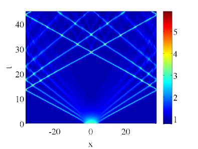
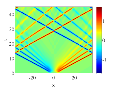
Figure 1.1: Dam-break results for the CH2 system in equations (1.11-1.12) show evolution of the density $\rho$ (left panel) and velocity $u$ (right panel), arising from initial conditions (1.16) in a periodic domain. The color bars show positive density on the left and both positive and negative velocity on the right. The soliton solutions are seen to emerge after a finite time, and the evolution of both variables generates more and more solitons propagating in both directions as time progresses. Figures are courtesy of L. Ó Náraigh.

Plan of the paper

Section 2 discusses the isospectral problem for the CH2 system. Section 3 treats asymptotics of the Jost solutions for the CH2 scattering problem. Section 4 explains how analytic solutions for CH2 are obtained by formulating the Inverse Scattering Transform (IST) for CH2 as a Riemann-Hilbert problem (RHP). Perhaps not unexpectedly from the viewpoint of CH2 as a fluids system, its solutions possess the parameterised form (4.15-4.17) corresponding to fluid continuum flow. Section 5 treats multi - soliton solutions of CH2 arising as reflectionless potentials. That is, the reflection coefficient in the inverse scattering transform is taken to vanish in the solution of the RHP for CH2. Section 6 provides a slightly modified CH2 equation that admits peakon solutions, but may not be integrable. Section 7 closes the paper by giving a brief summary of its main points and indicating some directions for future research.

2 The scattering problem for CH2

Outlook for the CH2 scattering problem.

This section begins our discussion of the isospectral problem for the two-component CH equation with a single velocity, denoted CH2 for simplicity. The next three short sections will be devoted to further discussions of the CH2 scattering problem. In §3, we will treat the asymptotics of the Jost solutions for the CH2 scattering problem. In §4, we will explain how to formulate the Inverse Scattering Transform for CH2 as a Riemann-Hilbert problem. Finally, in §5 we will derive multi - soliton solutions of CH2 that arise as reflectionless potentials.

2.1 CH2 spectral problem

The spectral problem for CH2 (1.9) is a type of Schrödinger equation with an ‘energy dependent’ potential. In particular, it is quadratic in the spectral parameter and the potential functions multiply the spectral parameter. (This is the so-called weighted problem.) It shares some features in common with Sturm-Liouville spectral problems, see for example [30, 33, 38]. An ‘energy dependent’ spectral problem also appears in the inverse scattering transform of an integrable generalization of the Bousinesq equation (Kaup-Bousinesq equation) [33].

Asymptotically, as $|x|\rightarrow\infty$, the spectral problem (1.9) for CH2 reduces to

$$\Psi_{xx} = \Big{(}-\rho_{0}^{2}\lambda^{2}+\omega\lambda+\frac{1}{4}\Big{)}\Psi,$$ (2.1)

or, simply

$$\Psi_{xx} = -k^{2}\Psi,$$ (2.2)

where we introduce a spectral parameter $k$ via the equation

$$-\rho_{0}^{2}\lambda^{2}+\omega\lambda+\frac{1}{4}+k^{2}=0,$$ (2.3)

The solutions of (2.2) oscillate for real $k$. Consequently, the continuous spectrum is the real line in the complex $k$-plane.

The quadratic equation (2.3) has roots,

$$\lambda(k,\sigma)=\frac{\omega}{2\rho_{0}^{2}}+\frac{\sigma k}{\rho_{0}}\sqrt{1+\frac{\rho_{0}^{2}+\omega^{2}}{4\rho_{0}^{2}k^{2}}},$$ (2.4)

where $\sigma=\pm 1$, and we assume $\sqrt{w}=\sqrt{|w|}e^{\frac{1}{2}Arg(w)}$ where $0\leq Arg(w)<2\pi$. An expansion of (2.4) for large $|k|$ yields,

$$\lambda(k,\sigma)=\frac{\sigma k}{\rho_{0}}+\frac{\omega}{2\rho_{0}^{2}}+\frac{\sigma(\rho_{0}^{2}+\omega^{2})}{8\rho_{0}^{3}}\frac{1}{k}+O\Big{(}\frac{1}{k^{3}}\Big{)}.$$ (2.5)

This expansion uniquely determines $\lambda$ from $k$ and $\sigma$. Equation (2.4) possesses a reflection property that we will assume explicitly from here on, that

$$\lambda(-k,-\sigma)=\lambda(k,\sigma),$$ (2.6)

and also, for real $k$,

$$\bar{\lambda}(k,\sigma)=\lambda(k,\sigma),$$ (2.7)

where $\bar{\lambda}$ is the complex conjugate.

As usual, for real $k\neq 0$ a basis in the space of solutions of (1.9) can be introduced, fixed by its asymptotic behavior when $x\rightarrow\infty$ [36, 7, 8]:

$$\psi_{1}(x,k) = e^{-ikx}+o(1),\qquad x\rightarrow\infty;$$ (2.8)

$$\psi_{2}(x,k) = e^{ikx}+o(1),\qquad x\rightarrow\infty.$$ (2.9)

A complementary basis can also be introduced, fixed by its asymptotic behavior when $x\rightarrow-\infty$:

$$\varphi_{1}(x,k) = e^{-ikx}+o(1),\qquad x\rightarrow-\infty;$$ (2.10)

$$\varphi_{2}(x,k) = e^{ikx}+o(1),\qquad x\rightarrow-\infty.$$ (2.11)

2.2 The scattering matrix, the Jost solutions and the reflection coefficient

Since $\lambda$ depends not only on $k$ but also on $\sigma$, it follows that the entire spectral problem, as well as the eigenfunctions, are labelled by $\sigma$. For all real $k\neq 0$, if $\Psi(x,k,\sigma)$ is a solution of (1.9), then $\Psi(x,-k,-\sigma)$ is also a solution, since they share the same $\lambda$, according to (2.6). Thus,

$$\varphi_{1}(x,k,\sigma)=\varphi_{2}(x,-k,-\sigma),\qquad\psi_{1}(x,k,\sigma)=\psi_{2}(x,-k,-\sigma).$$ (2.12)

Due to the reality of $q$, $\rho$ in (1.9) and the property (2.7) for $\lambda$, for real $k$ we have

$$\varphi_{1}(x,k,\sigma)=\bar{\varphi}_{2}(x,k,\sigma),\qquad\psi_{1}(x,k,\sigma)=\bar{\psi}_{2}(x,k,\sigma).$$ (2.13)

For real $k$ the vectors of each of the bases may be represented as a linear combination of the vectors of the other basis:

$$\varphi_{i}(x,k,\sigma)=\sum_{l=1,2}T_{il}(k,\sigma)\psi_{l}(x,k,\sigma),$$ (2.14)

where the matrix $T(k,\sigma)$ defined above is called the scattering matrix.

For real $k\neq 0$, instead of $\varphi_{1}(x,k,\sigma)$ and $\varphi_{2}(x,k,\sigma)$, due to (2.13), for simplicity we can write correspondingly $\varphi(x,k,\sigma)$, $\bar{\varphi}(x,k,\sigma)$. Similarly, we can replace $\psi_{1,2}(x,k,\sigma)$ by $\psi(x,k,\sigma)$ and its complex conjugate $\bar{\psi}(x,k,\sigma)$. Thus $T(k,\sigma)$ has the form (with real $k$)

$$T(k,\sigma)=\left(\begin{array}[]{cc}a(k,\sigma)&b(k,\sigma)\\ \bar{b}(k,\sigma)&\bar{a}(k,\sigma)\\ \end{array}\right)\,$$ (2.17)

and clearly

$$\varphi(x,k,\sigma)=a(k,\sigma)\psi(x,k,\sigma)+b(k,\sigma)\bar{\psi}(x,k,\sigma).$$ (2.18)

Remark. The solutions $\varphi(x,k,\sigma)$ and $\psi(x,k,\sigma)$ are called the Jost solutions.

The Wronskian $W(f_{1},f_{2})\equiv f_{1}\partial_{x}f_{2}-f_{2}\partial_{x}f_{1}$ of any pair of solutions of (1.9) does not depend on $x$. Therefore, perhaps not unexpectedly,

$$W(\varphi(x,k,\sigma),\bar{\varphi}(x,k,\sigma))=W(\psi(x,k,\sigma),\bar{\psi}(x,k,\sigma))=2ik.$$ (2.19)

From (2.18) and (2.19) it follows that

$$|a(k,\sigma)|^{2}-|b(k,\sigma)|^{2}=1.$$ (2.20)

Hence, $\det(T(k,\sigma))=1$. That is, the determinant of the scattering matrix is unity.

In analogy with the spectral problem for the KdV equation, (which is the Schrödinger equation from quantum mechanics) [36], one can introduce a reflection coefficient,

$$\mathcal{R}(k,\sigma)=b(k,\sigma)/a(k,\sigma).$$ (2.21)

The matrix $T(k,\sigma)$ in (2.17) is determined from the knowledge of $\mathcal{R}(k,\sigma)$ for real $k>0$ only. Indeed, from (2.12) we have $\psi(x,k,\sigma)=\bar{\psi}(x,-k,-\sigma)$, etc. for real $k$. Hence, the scattering data satisfy

$$\bar{a}(k,\sigma)=a(-k,-\sigma),\qquad\bar{b}(k,\sigma)=b(-k,-\sigma).$$ (2.22)

Also, it is sufficient to know $\mathcal{R}(k,\sigma)$ only on the half line $k>0$, since $\mathcal{R}(-k,-\sigma)=\bar{\mathcal{R}}(k,\sigma)$.

3 Asymptotics of the Jost solutions for CH2 as $|k|\to\infty$

Outlook.

This section continues the analysis of the CH2 scattering problem, by discussing the asymptotic behavior of the Jost solutions.

3.1 Analyticity properties

The analyticity properties of the Jost solutions and of $a(k,\sigma)$ play an important role in our considerations. We will need also the asymptotic behavior of the Jost solutions for $|k|\rightarrow\infty$ which have the form (cf. [8, 9])

$$\psi(x,k,\sigma)=e^{-ikx-ik\int_{\infty}^{x}(\frac{\rho(x^{\prime})}{\rho_{0}}-1)dx^{\prime}+i\frac{\sigma}{2}\int_{\infty}^{x}(\frac{q(x^{\prime})}{\rho(x^{\prime})}-\frac{\omega\rho(x^{\prime})}{\rho_{0}^{2}})dx^{\prime}}\left[X_{0}(x)+O\left(\frac{1}{k}\right)\right],$$

(3.1)

$$\varphi(x,k,\sigma)=e^{-ikx-ik\int_{-\infty}^{x}(\frac{\rho(x^{\prime})}{\rho_{0}}-1)dx^{\prime}+i\frac{\sigma}{2}\int_{-\infty}^{x}(\frac{q(x^{\prime})}{\rho(x^{\prime})}-\frac{\omega\rho(x^{\prime})}{\rho_{0}^{2}})dx^{\prime}}\left[X_{0}(x)+O\left(\frac{1}{k}\right)\right],$$

(3.2)

where $X_{0}(x)=\left(\frac{\rho_{0}}{\rho(x)}\right)^{1/2}$. (If initially $\rho(x,0)>0$, one can easily prove that $\rho(x,t)$ always remains positive.) As in [8] one can show that $\psi(x,k,\sigma)$ is analytic in the lower complex half $k$ -plane, while $\varphi(x,k,\sigma)$ is analytic in the upper complex half $k$ -plane.

The expression for $a(k,\sigma)$ can be extended into the upper half plane by

$$a(k,\sigma)=\frac{1}{2ik}W(\varphi(x,k,\sigma),\psi(x,-k,-\sigma)).$$ (3.3)

An immediate consequence of (3.1), (3.2) and (3.3) is:

$$\lim_{k\to\infty}a(k,\sigma)e^{ik\alpha-i\sigma\beta}=1,\qquad k\in{\mathbb{C}}_{+},$$ (3.4)

where the quantities

$$\alpha = \int_{-\infty}^{\infty}\left(\frac{\rho(x)}{\rho_{0}}-1\right)\text{d}x,$$ (3.5)

$$\beta = \frac{1}{2}\int_{-\infty}^{\infty}\left(\frac{q(x)}{\rho(x)}-\frac{\omega\rho(x)}{\rho_{0}^{2}}\right)dx,$$ (3.6)

are two integrals of the system, [28].

3.2 The discrete spectrum.

The discrete spectrum can be found as follows. Suppose that $k_{0}(\sigma)\in{\mathbb{C}}_{+}$ is a zero of $a(k,\sigma)$. Then $\varphi(x,k_{0},\sigma)$ and $\psi(x,-k_{0},-\sigma)$ are linearly dependent (2.18):

$$\varphi(x,k_{0},\sigma)=b_{0}(\sigma)\psi(x,-k_{0},-\sigma).$$ (3.7)

From here we see that $\varphi(x,k_{0},\sigma)$ decays exponentially for both $x\rightarrow-\infty$ (which follows from the definition of $\varphi(x,k_{0},\sigma)$) and $x\rightarrow+\infty$ (since $\psi(x,-k_{0},-\sigma)=e^{ikx}$ for $x\rightarrow\infty$). Therefore $\varphi(x,k_{0},\sigma)$ is a well defined eigenfunction of the discrete spectrum with an eigenvalue $k_{0}$.

Now, multiplying (1.9) by $\bar{\varphi}(x,k_{0},\sigma)$ and performing some manipulations while keeping in mind that the eigenfunction decays exponentially for both $x\rightarrow\pm\infty$, we obtain

$$\lambda^{2}(k_{0})\int_{-\infty}^{\infty}q_{2}(x)|\varphi|^{2}\text{d}x+\lambda(k_{0})\int_{-\infty}^{\infty}q_{1}(x)|\varphi|^{2}\text{d}x+$$

$$\int_{-\infty}^{\infty}\Big{(}\frac{1}{4}|\varphi|^{2}+|\varphi_{x}|^{2}\Big{)}\text{d}x=0$$ (3.8)

This identity can be regarded as an equation for $\lambda(k_{0})$ where $k_{0}$ is a parameter. From the quadratic formula, the two roots $\lambda(k_{0},\sigma)$ and $\lambda(k_{0},-\sigma)$ satisfy

$$\lambda(k_{0},\sigma)\lambda(k_{0},-\sigma)=-\,\frac{\int_{-\infty}^{\infty}\Big{(}\frac{1}{4}|\varphi|^{2}+|\varphi_{x}|^{2}\Big{)}\text{d}x}{\int_{-\infty}^{\infty}\rho^{2}(x)|\varphi|^{2}\text{d}x}\,.$$ (3.9)

On the other hand, from (2.3) we have

$$\lambda(k_{0},\sigma)\lambda(k_{0},-\sigma)=-\frac{1}{\rho_{0}^{2}}\Big{(}k_{0}^{2}+\frac{1}{4}\Big{)}.$$ (3.10)

From (3.9) and (3.10) it follows that $k_{0}^{2}+\frac{1}{4}$ is real and positive. Since $k_{0}$ is in the upper half complex plane, it should be exactly on the imaginary axis, $k_{0}=i\kappa_{0}$, where $\kappa_{0}$ is real, and $0<\kappa_{0}<1/2$. With this restriction on $k_{0}$, notice that $\lambda(k_{0},\sigma)$ is real.

Let us show that $a(k,\sigma)$ can have only simple zeroes in the upper half complex plane. The dot will be used to denote the derivatives with respect to $k$ at the point $k_{0}$. From (2.3) we have $\dot{\lambda}=2k/(2\rho_{0}^{2}\lambda-\omega)$. Differentiating the (1.9) (written for the eigenfunction $\varphi$) with respect to $k$ and multiplying by $\bar{\varphi}$ we obtain

$$(\bar{\varphi}\dot{\varphi}_{x}-\bar{\varphi}_{x}\dot{\varphi})|_{-\infty}^{\infty}=\dot{\lambda}\int_{-\infty}^{\infty}(q-2\lambda\rho^{2})|\varphi|^{2}\text{d}x.$$ (3.11)

Next, using the asymptotics $\dot{\varphi}(x,k_{0},\sigma)\rightarrow\dot{a}(k_{0},\sigma)e^{\kappa_{0}x}$, $\varphi(x,k_{0},\sigma)\rightarrow b_{0}(\sigma)e^{-\kappa_{0}x}$ for $x\rightarrow\infty$; $\dot{\varphi}(x,k_{0},\sigma)\rightarrow 0$, $\varphi(x,k_{0},\sigma)\rightarrow 0$ for $x\rightarrow-\infty$, (3.11) can be transformed into

$$\int_{-\infty}^{\infty}(q-2\lambda(k_{0})\rho^{2})|\varphi|^{2}\text{d}x=(\omega-2\rho_{0}^{2}\lambda(k_{0}))i\bar{b}_{0}\dot{a}(k_{0}).$$ (3.12)

As a corollary we notice that the quantity $R_{0}(\sigma,t)=\frac{b_{0}}{i\dot{a}(k_{0})}$ is real.

If $\int_{-\infty}^{\infty}(q-2\lambda(k_{0})\rho^{2})|\varphi|^{2}\text{d}x\neq 0$, then $\dot{a}(k_{0})\neq 0$ and the zero $k_{0}$ is simple. Therefore, a multiple zero is possible, only if

$$\int_{-\infty}^{\infty}(q-2\lambda(k_{0})\rho^{2})|\varphi|^{2}\text{d}x=0.$$ (3.13)

Suppose that (3.13) is satisfied. From (1.9) (written for the eigenfunction $\varphi$) multiplied by $\bar{\varphi}$ we obtain

$$-\lambda^{2}(k_{0})\int_{-\infty}^{\infty}\rho^{2}(x)|\varphi|^{2}\text{d}x + \lambda(k_{0})\int_{-\infty}^{\infty}q(x)|\varphi|^{2}\text{d}x$$ (3.14)

$$+\int_{-\infty}^{\infty}\Big{(}\frac{1}{4}|\varphi|^{2}+|\varphi_{x}|^{2}\Big{)}\text{d}x=0.$$

From (3.13) and (3.14) we obtain

$$\lambda(k_{0})^{2}=-\frac{\int_{-\infty}^{\infty}\Big{(}\frac{1}{4}|\varphi|^{2}+|\varphi_{x}|^{2}\Big{)}\text{d}x}{\int_{-\infty}^{\infty}\rho^{2}(x)|\varphi|^{2}\text{d}x},$$ (3.15)

but from $(\ref{identityforlambdak0})$ itself we find that the product of the two roots is

$$\lambda(k_{0},\sigma)\lambda(k_{0},-\sigma)=-\frac{\int_{-\infty}^{\infty}\Big{(}\frac{1}{4}|\varphi|^{2}+|\varphi_{x}|^{2}\Big{)}\text{d}x}{\int_{-\infty}^{\infty}\rho^{2}(x)|\varphi|^{2}\text{d}x}.$$ (3.16)

From (3.15), (3.16) and (2.4) we find that $\lambda(k_{0},\sigma)=\lambda(k_{0},-\sigma)=\frac{\omega}{2\rho_{0}^{2}}$. Thus in this case the multiplier $\omega-2\rho_{0}^{2}\lambda(k_{0})$ on the right hand side of (3.12) is also zero. Therefore, we can use l’Hospital’s rule in the evaluation of $\dot{a}(k_{0})$. From (3.12) we have

$$\dot{a}(k_{0}) = \lim_{\lambda\rightarrow\frac{\omega}{2\rho_{0}^{2}}}\frac{\frac{\partial}{\partial\lambda}\int_{-\infty}^{\infty}(q-2\lambda\rho^{2})|\varphi|^{2}\text{d}x}{i\bar{b}_{0}\frac{\partial}{\partial\lambda}(\omega-2\lambda\rho_{0}^{2})}$$ (3.17)

$$= \lim_{\lambda\rightarrow\frac{\omega}{2\rho_{0}^{2}}}\frac{-2\int_{-\infty}^{\infty}\rho^{2}|\varphi|^{2}\text{d}x+2\frac{\partial k}{\partial\lambda}\int_{-\infty}^{\infty}(q-2\lambda\rho^{2})|\varphi||\dot{\varphi}|\text{d}x}{-2i\bar{b}_{0}\rho_{0}^{2}}$$

$$= \frac{\int_{-\infty}^{\infty}\rho^{2}|\varphi|^{2}\text{d}x}{i\bar{b}_{0}\rho_{0}^{2}},$$

since

$$\lim_{\lambda\rightarrow\frac{\omega}{2\rho_{0}^{2}}}\frac{\partial k}{\partial\lambda}=\lim_{\lambda\rightarrow\frac{\omega}{2\rho_{0}^{2}}}\frac{2\rho_{0}^{2}\lambda-\omega}{2k}=0.$$

Then (3.17) shows that $\dot{a}(k_{0})\neq 0$, i.e. $k_{0}$ is a simple zero of $a(k)$.

3.3 Summary of asymptotic behavior of Jost functions for CH2

To summarize: the discrete spectrum in the upper half plane consists of finitely many points $k_{n}=i\kappa_{n}$, $n=1,\ldots,N$, which are the simple zeroes of $a(k,\sigma)$. Furthermore, each $\kappa_{n}$ is real and $0<\kappa_{n}<1/2$.

Eigenfunctions.

Two eigenfunctions $\varphi^{(n)}(x,\sigma)$ belong to each eigenvalue $i\kappa_{n}$, because there are two eigenvalues $\lambda_{n}(\sigma)=\lambda(i\kappa_{n},\sigma)$ that correspond to a given $\kappa_{n}$. We can take this eigenfunction to be

$$\varphi^{(n)}(x,\sigma)\equiv\varphi(x,i\kappa_{n},\sigma)\,.$$ (3.18)

The asymptotic behavior of $\varphi^{(n)}$, according to (2.10), (2.9), (3.7) is

$$\varphi^{(n)}(x,\sigma) = e^{\kappa_{n}x}+o(e^{\kappa_{n}x})\quad\hbox{for}\quad x\rightarrow-\infty\,,$$ (3.19)

$$\varphi^{(n)}(x,\sigma) = b_{n}(\sigma)e^{-\kappa_{n}x}+o(e^{-\kappa_{n}x})\quad\hbox{for}\quad x\rightarrow\infty.$$ (3.20)

Scattering data.

The set

$$\mathcal{S}\equiv\{\mathcal{R}(k,\sigma)\quad(k>0),\quad\kappa_{n},\quad b_{n}(\sigma),\quad n=1,\ldots N,\quad\sigma=\pm 1\},$$ (3.21)

is called the scattering data.

The time evolution of the scattering data can be easily obtained as follows.

The second equation of the Lax pair is

$$\Psi_{t} = \Big{(}\frac{1}{2\lambda}-u\Big{)}\Psi_{x}+\frac{u_{x}}{2}\Psi+\gamma\Psi,$$ (3.22)

where we introduced an arbitrary constant $\gamma$ (which does not affect the compatibility).

From (2.18) with $x\rightarrow\infty$ one has

$$\varphi(x,k,\sigma)=a(k,\sigma)e^{-ikx}+b(k,\sigma)e^{ikx}+o(1).$$ (3.23)

The substitution of $\varphi(x,k,\sigma)$ into (3.22) with $x\rightarrow\infty$ gives

$$\varphi_{t}=\frac{1}{2\lambda}\varphi_{x}+\gamma\varphi\,.$$ (3.24)

From (3.23), (3.24) with the choice $\gamma=ik/2\lambda$ for the eigenfunction $\varphi(x,k)$ we obtain

$$a_{t}(k,\sigma,t) = 0,$$ (3.25)

$$b_{t}(k,t,\sigma) = \frac{ik}{\lambda}b(k,t,\sigma).$$ (3.26)

Thus, we find

$$a(k,t,\sigma)=a(k,0,\sigma),\qquad b(k,t,\sigma)=b(k,0,\sigma)e^{\frac{ik}{\lambda}t},$$ (3.27)

$$\mathcal{R}(k,t,\sigma)=\mathcal{R}(k,0,\sigma)e^{\frac{ik}{\lambda(k,\sigma)}t}.$$ (3.28)

In other words, $a(k,\sigma)$ does not depend on $t$ and can serve as a generating function of the conservation laws.

Time evolution of the data on the discrete spectrum.

The time evolution of the data on the discrete spectrum is found as follows. Let us introduce the notation $\dot{a}_{n}(\sigma)\equiv\dot{a}(i\kappa_{n},\sigma)$. We notice that $i\kappa_{n}$ are zeroes of $a(k,\sigma)$, which does not depend on $t$, and hence $(\kappa_{n})_{t}=0$ and $\lambda_{n}(\sigma)_{t}=0$. From (3.22), (2.4) with $\gamma=ik/2\lambda$; $k=i\kappa_{n}$ and (3.20) one can obtain

$$b_{n}(\sigma)_{t}=\frac{-\kappa_{n}}{\lambda_{n}(\sigma)}b_{n}(\sigma).$$ (3.29)

It is convenient to use the variable $R_{n}(\sigma)\equiv\frac{b_{n}(\sigma)}{i\dot{a}_{n}(\sigma)}$, which is real, according to (3.12) and evolves with $t$ as

$$R_{n}(t,\sigma)=R_{n}(0,\sigma)\exp\Big{(}\frac{-\kappa_{n}}{\lambda_{n}(\sigma)}t\Big{)}.$$ (3.30)

When $k$ is in the upper half plane one can derive the following dispersion relation for $a(k,\sigma)$ e.g. following the pattern for the CH case from [9]:

$$\ln a(k,\sigma)=-i\alpha k+i\sigma\beta+\sum_{n=1}^{N}\ln\frac{k-i\kappa_{n}}{k+i\kappa_{n}}+\frac{1}{\pi i}\int_{-\infty}^{\infty}\frac{\ln|a(k^{\prime},\sigma)|}{k^{\prime}-k}dk^{\prime},$$ (3.31)

i.e. $a(k,\sigma)$ is determined by $|a(k,\sigma)|$ given on the real line $k\in\mathbb{R}$.

Outlook.

In the next section, we will develop the Inverse Scattering Transform for CH2. The special case of reflectionless potentials ($\mathcal{R}(k,\sigma)=0$ for all $k$) corresponds to an important class of solutions, namely the multi-soliton solutions. These will be separately studied in Section 5, where a formula for the $N$-soliton solution will be obtained.

4 Analytic solutions and the Riemann-Hilbert Problem for CH2

This section explains how analytic solutions for CH2 are obtained by formulating the Inverse Scattering Transform for CH2 as a Riemann-Hilbert problem (RHP).

4.1 Preliminaries

We begin by introducing the following new variables, cf. the integrals of motion in equation (3.5) and (3.6)

$$y(x) = x+\int_{\infty}^{x}\left(\frac{\rho(x^{\prime})}{\rho_{0}}-1\right)\text{d}x^{\prime},$$ (4.1)

$$z(x) = \frac{1}{2}\int_{\infty}^{x}\left(\frac{q(x^{\prime})}{\rho(x^{\prime})}-\frac{\omega\rho(x^{\prime})}{\rho_{0}^{2}}\right)\text{d}x^{\prime}.$$ (4.2)

In terms of these variables, the expansion (3.1) may be written as

$$\psi(x,k,\sigma)=e^{-iky+i\sigma z}\left[X_{0}(x)+O\left(\frac{1}{k}\right)\right].$$ (4.3)

Furthermore, the function $\underline{\chi}(x,k,\sigma)\equiv\psi(x,k,\sigma)e^{ikx}$ is analytic for $\mathrm{Im}\phantom{*}k<0$, due to arguments similar to these, given in [7] for the CH case. This follows from the representation

$$\underline{\chi}(x,k)=1-\int_{x}^{\infty}\frac{e^{2ik(x-x^{\prime})}-1}{2ik}[-\lambda^{2}(\rho^{2}(x^{\prime})-\rho_{0}^{2})+\lambda(q(x^{\prime})-\omega))]\,\underline{\chi}(x^{\prime},k)dx^{\prime}.$$

Notice that $y(x)$ is a bounded function for all $x$, which follows from the assumption that $\rho(x)-\rho_{0}$ is a Schwartz class function. Therefore, the function

$$\underline{\psi}(x,k,\sigma)\equiv\psi(x,k,\sigma)e^{iky-i\sigma z}=X_{0}(x)+O\left(\frac{1}{k}\right)$$ (4.4)

is also analytic for $\mathrm{Im}\phantom{*}k<0$.

Similarly,

$$\underline{\varphi}(x,k,\sigma) \equiv \varphi(x,k,\sigma)e^{iky-i\sigma z+ik\alpha-i\sigma\beta}=X_{0}(x)+O\left(\frac{1}{k}\right)$$ (4.5)

is analytic for $\mathrm{Im}\phantom{*}k>0$.

Multiplying (2.18) by $e^{iky-i\sigma z}/a(k,\sigma)$ and using (4.4) and (4.5) we obtain

$$\frac{\underline{\varphi}(x,k,\sigma)}{e^{ik\alpha-i\sigma\beta}a(k,\sigma)}=\underline{\psi}(x,k,\sigma)+\mathcal{R}(k,\sigma)\underline{\psi}(x,-k,-\sigma)e^{2iky-2i\sigma z}.$$ (4.6)

The function $\frac{\underline{\varphi}(x,k,\sigma)}{e^{ik\alpha-i\sigma\beta}a(k,\sigma)}$ is analytic for $\mathrm{Im}\phantom{*}k>0$, while $\underline{\psi}(x,k,\sigma)$ is analytic for $\mathrm{Im}\phantom{*}k<0$. Thus, equation (4.6) represents an additive Riemann-Hilbert Problem (RHP) with a jump on the real line, given by $\mathcal{R}(k,\sigma)\underline{\psi}(x,-k,-\sigma)e^{2iky-2i\sigma z}$ and a normalization condition, $\lim_{|k|\to\infty}\underline{\psi}(x,k,\sigma)=X_{0}(x)$.

4.2 Solving the Riemann-Hilbert Problem for CH2

In this section we will follow the standard technique for solving RHP. We integrate the two analytic functions with respect to $\oint\frac{dk^{\prime}}{k^{\prime}-k}(\cdot)$ over the boundary of their analyticity domains, using the normalization condition. In our case the domains (the upper $\mathbb{C}_{+}$ and the lower $\mathbb{C}_{-}$ complex half-planes) have the real line as a common boundary and there we relate the integrals using the jump condition. The RHP approach for the CH equation is presented in [8, 2, 19], for the Kaup-Bousinesq equation (which also has energy-dependent spectal problem) in [38].

Let us take an arbitrary $k$ from the lower half plane ($\mathrm{Im}\phantom{*}k<0$). Then using the Residue Theorem, (3.5) and (3.7) we can compute the integral

$$I = \frac{1}{2\pi i}\oint_{C_{+}}\frac{\underline{\varphi}(x,k^{\prime},\sigma)}{e^{ik^{\prime}\alpha-i\sigma\beta}a(k^{\prime},\sigma)}\frac{dk^{\prime}}{k^{\prime}-k}$$ (4.7)

$$= \sum_{n=1}^{N}\frac{\underline{\varphi}(x,i\kappa_{n},\sigma)}{(i\kappa_{n}-k)e^{-\kappa_{n}\alpha-i\sigma\beta}\dot{a}_{n}(\sigma)}$$

$$= \sum_{n=1}^{N}\frac{iR_{n}(\sigma)e^{-2\kappa_{n}y-2i\sigma z}\underline{\psi}(x,-i\kappa_{n},-\sigma)}{i\kappa_{n}-k},$$

where $C_{+}$ is the closed contour in the upper half plane (Fig. 4.1).

Figure 4.1: The contours $\Gamma_{\pm}$

On the other hand, because of (4.6) the same integral can be computed directly as

$$I = \frac{1}{2\pi i}\int_{-\infty}^{\infty}\left(\underline{\psi}(x,k^{\prime},\sigma)+\mathcal{R}(k^{\prime},\sigma)\underline{\psi}(x,-k^{\prime},-\sigma)e^{2ik^{\prime}y-2i\sigma z}\right)\frac{dk^{\prime}}{k^{\prime}-k}$$ (4.8)

$$+ \frac{1}{2\pi i}\int_{\Gamma_{+}}\frac{\underline{\varphi}(x,k^{\prime},\sigma)}{e^{ik^{\prime}\alpha-i\sigma\beta}a(k^{\prime},\sigma)}\frac{dk^{\prime}}{k^{\prime}-k},$$

where $\Gamma_{+}$ is the infinite semicircle in the upper half plane (Fig. 4.1). Using the expansion (4.5) and limit (3.4), it is straightforward to compute that the integral over $\Gamma_{+}$ is simply $(1/2)X_{0}(x)$.

Similarly,

$$-\underline{\psi}(x,k,\sigma) = \frac{1}{2\pi i}\oint_{C_{-}}\underline{\psi}(x,k^{\prime},\sigma)\frac{dk^{\prime}}{k^{\prime}-k}=\frac{1}{2\pi i}\int_{-\infty}^{\infty}\underline{\psi}(x,k^{\prime},\sigma)\frac{dk^{\prime}}{k^{\prime}-k}$$ (4.9)

$$+ \frac{1}{2\pi i}\int_{\Gamma_{-}}\underline{\psi}(x,k^{\prime},\sigma)\frac{dk^{\prime}}{k^{\prime}-k},$$

where $C_{-}$ is the closed contour in the lower half plane, $\Gamma_{-}$ is the infinite semicircle in the lower half plane (Fig. 4.1). Due to (4.3), (4.4) the integral over $\Gamma_{-}$ is $-(1/2)X_{0}(x)$.

Now, from (4.7) – (4.9) it follows that for $\mathrm{Im}\phantom{*}k<0$,

$$\underline{\psi}(x,k,\sigma) = X_{0}(x)+\int_{-\infty}^{\infty}\mathcal{R}(k^{\prime},\sigma)\underline{\psi}(x,-k^{\prime},-\sigma)e^{2ik^{\prime}y-2i\sigma z}\frac{dk^{\prime}}{k^{\prime}-k}$$ (4.10)

$$+ \sum_{n=1}^{N}\frac{iR_{n}(\sigma)e^{-2\kappa_{n}y-2i\sigma z}\underline{\psi}(x,-i\kappa_{n},-\sigma)}{k-i\kappa_{n}}.$$

The expression (4.10), taken at $k=-i\kappa_{p}$, $p=1,\ldots,N$ gives

$$\underline{\psi}(x,-i\kappa_{p},\sigma) = X_{0}(x)$$ (4.11)

$$+ \int_{-\infty}^{\infty}\mathcal{R}(k^{\prime},\sigma)\underline{\psi}(x,-k^{\prime},-\sigma)e^{2ik^{\prime}y-2i\sigma z}\frac{dk^{\prime}}{k^{\prime}+i\kappa_{p}}$$

$$- \sum_{n=1}^{N}\frac{R_{n}(\sigma)e^{-2\kappa_{n}y-2i\sigma z}\underline{\psi}(x,-i\kappa_{n},-\sigma)}{\kappa_{p}+\kappa_{n}}.$$

From (4.11) it follows immediately that

$$\underline{\psi}(x,-i\kappa_{p},-\sigma) = X_{0}(x)$$

$$+ \int_{-\infty}^{\infty}\mathcal{R}(k^{\prime},-\sigma)\underline{\psi}(x,-k^{\prime},\sigma)e^{-2ik^{\prime}y+2i\sigma z}\frac{dk^{\prime}}{k^{\prime}+i\kappa_{p}}$$

$$- \sum_{n=1}^{N}\frac{R_{n}(-\sigma)e^{-2\kappa_{n}y+2i\sigma z}\underline{\psi}(x,-i\kappa_{n},\sigma)}{\kappa_{p}+\kappa_{n}}.$$

Equations (4.10) – (LABEL:eq34a) represent a linear system, from which $\underline{\psi}(x,k,\sigma)$ (for real $k$) and $\underline{\psi}(x,-i\kappa_{n},\pm\sigma)$ can be expressed through $y$, $z$, which are as yet unknown functions of $x$ (since $X_{0}(x)$ can be obtained from $y(x)$).

Finally, we need to find the dependence of $y$ on $x$. From the quadratic roots in (2.4) we notice that

$$\lambda(-i/2,\sigma)=\frac{\omega-\sigma|\omega|}{2\rho_{0}^{2}}.$$

Hence, if we take $\sigma=\sigma_{1}\equiv\text{sign}(\omega)$, then we have $\lambda(-i/2,\sigma_{1})=0$. Now $\psi(x,k,\sigma_{1})$ does not depend on $q$ and $\rho$ for $\lambda=0$ and since $\psi(x,k,\sigma_{1})$ is defined by its asymptotic behavior as $x\to\infty$, which is $e^{-x/2}$, i.e., it is real when $k=-i/2$. Consequently, we have

$$\frac{1}{2}\left(\psi(x,-i/2,\sigma_{1})+\text{compl. conj.}\right)=e^{-x/2}.$$

Thus, for $k=-i/2$, $\sigma=\sigma_{1}\equiv\text{sign}(\omega_{1})$, equation (4.10) gives

$$e^{(-x+y)/2} = e^{i\sigma_{1}z}\Big{(}X_{0}(x)+\int_{-\infty}^{\infty}\mathcal{R}(k^{\prime},\sigma_{1})\underline{\psi}(x,-k^{\prime},-\sigma_{1})e^{2ik^{\prime}y-2i\sigma_{1}z}\frac{dk^{\prime}}{k^{\prime}+i/2}$$ (4.13)

$$- \sum_{n=1}^{N}\frac{R_{n}(\sigma_{1})e^{-2\kappa_{n}y-2i\sigma_{1}z}\underline{\psi}(x,-i\kappa_{n},-\sigma_{1})}{1/2+\kappa_{n}}\Big{)}+\text{complex conjugate}$$

In other words, (4.10) – (4.13) represent a system of singular integral equations for $\underline{\psi}(x,k,\sigma)$ (for real $k$) and $\underline{\psi}(x,-i\kappa_{n}(\sigma),\sigma)$, $\underline{\bar{\psi}}(x,-i\kappa_{n}(\sigma),\sigma)$.

A similar relation to (4.10) can be written if $k\in\mathbb{C}_{+}$ and in particular when $k=i/2$ we have another equation of the type of (4.13). Thus, one can recover

$$x=X(y,z(y))\quad\hbox{and}\quad\frac{dx}{dy}\equiv X_{0}^{2}(y,z(y)).$$ (4.14)

Then eliminating $z$ eventually yields $x=X(y)$.

Parametric forms of the solutions.

Since the time evolution of the scattering data is known (3.30), the dependence on $t$, i.e. $x=X(y,t)$, is also known, as expressed by the scattering data. Thus the set $\mathcal{S}$ of scattering data (3.21) uniquely determines the solution. From (4.1) one obtains the parametric forms of the solutions,

$$x = X(y,t),$$ (4.15)

$$\rho(x,t) = \frac{\rho_{0}}{X_{y}(y,t)},$$ (4.16)

$$u(x,t) = X_{t}(y,t).$$ (4.17)

These correspond precisely to the relations between Eulerian and Lagrangian variables in compressible ideal fluid dynamics.

5 Reflectionless potentials and solitons for CH2

This section discusses the simplification of the inverse scattering problem for CH2 in the important case of the so-called reflectionless potentials, when the scattering data is confined to the case $\mathcal{R}(k,\sigma)=0$ for all real $k$. This class of potentials corresponds to the multi - soliton solutions of the two component CH equation.

The time evolution of $R_{n}$ due to (3.30) is

$$R_{n}(t,\sigma)=R_{n}(0,\sigma)\exp\left(\frac{-\kappa_{n}}{\lambda_{n}(\sigma)}t\right).$$ (5.1)

As we already observed, both $\lambda_{n}(\sigma)$ and $R_{n}(t,\sigma)$ are real. Let us define the $N\times N$ matrix

$$M_{pq}(y,t,\sigma)=\delta_{pq}-\sum_{n=1}^{N}\frac{R_{n}(t,\sigma)R_{q}(t,-\sigma)e^{-2y(\kappa_{n}+\kappa_{q})}}{(\kappa_{p}+\kappa_{n})(\kappa_{n}+\kappa_{q})},$$ (5.2)

which is real, and the vectors (with real components)

$$A_{n}(y,t,\sigma) = \sum_{p=1}^{N}[M^{-1}(y,t,\sigma)]_{np},$$ (5.3)

$$B_{n}(y,t,\sigma) = \sum_{p=1}^{N}\sum_{q=1}^{N}[M^{-1}(y,t,\sigma)]_{np}\frac{R_{q}(t,\sigma)e^{-2y\kappa_{q}}}{\kappa_{p}+\kappa_{q}}.$$ (5.4)

The solution of the system (4.11), (LABEL:eq34a) is

$$\underline{\psi}(x,-i\kappa_{n},\sigma) = X_{0}(x)[A_{n}(y,t,\sigma)-e^{-2i\sigma z}B_{n}(y,t,\sigma)],$$ (5.5)

and from (4.10) also

$$\underline{\psi}(x,k,\sigma) = X_{0}(x)\Big{[}1-\sum_{n=1}^{N}\frac{iR_{n}(t,\sigma)e^{-2\kappa_{n}y}B_{n}(y,t,-\sigma)}{k-i\kappa_{n}}$$ (5.6)

$$\hskip 5.69054pt+\ e^{-2i\sigma z}\sum_{n=1}^{N}\frac{iR_{n}(t,\sigma)e^{-2\kappa_{n}y}A_{n}(y,t,-\sigma)}{k-i\kappa_{n}}\Big{]}.$$

From (4.13) we have

$$e^{(-x+y)/2} = \cos(\sigma_{1}z)X_{0}(x)\Big{(}1-\sum_{n=1}^{N}\frac{R_{n}(\sigma_{1})e^{-2\kappa_{n}y}(A_{n}(y,t,-\sigma_{1})-B_{n}(y,t,-\sigma_{1}))}{\kappa_{n}+1/2}\Big{)}.$$

A similar relation for $\underline{\varphi}(x,k,\sigma)$ can be written if $k\in\mathbb{C}_{+}$ and for $k=i/2$ it gives

$$e^{(x-y)/2} = \cos(\sigma_{1}z)X_{0}(x)\Big{(}1-\sum_{n=1}^{N}\frac{R_{n}(-\sigma_{1})e^{-2\kappa_{n}y}(A_{n}(y,t,\sigma_{1})-B_{n}(y,t,\sigma_{1}))}{\kappa_{n}-1/2}\Big{)},$$

and finally from (LABEL:eq:xy1) and (LABEL:eq:xy2):

$$x \equiv X(y,t)=y+\ln\frac{f_{-}(y,t)}{f_{+}(y,t)}\,,$$ (5.9)

$$f_{\pm}(y,t) = 1-\sum_{n=1}^{N}\frac{R_{n}(\pm\sigma_{1})e^{-2\kappa_{n}y}(A_{n}(y,t,\mp\sigma_{1})-B_{n}(y,t,\mp\sigma_{1}))}{\kappa_{n}\pm 1/2}\,.$$ (5.10)

The time evolution of $R_{n}$ is known (5.1) and thus $X(y,t)$ is given in terms of the scattering data. This produces a parametric representation of the solution in terms of the dependent variables, from equations (4.15) – (4.17).

For the one-soliton solution, equations (5.9) and (5.10) yield the parametric (Lagrangian) representation of the “particle paths”,

$$X(y,t)=y+\ln\frac{1-\frac{\frac{1}{2}+\kappa_{1}}{\frac{1}{2}-\kappa_{1}}E(\sigma_{1})E(-\sigma_{1})+\frac{2\kappa_{1}}{\frac{1}{2}-\kappa_{1}}E(-\sigma_{1})}{1-\frac{\frac{1}{2}-\kappa_{1}}{\frac{1}{2}+\kappa_{1}}E(\sigma_{1})E(-\sigma_{1})-\frac{2\kappa_{1}}{\frac{1}{2}+\kappa_{1}}E(\sigma_{1})},$$ (5.11)

where $E(\sigma,t)=\frac{1}{2\kappa_{1}}R_{1}(t,\sigma)e^{-2\kappa_{1}y}$.

We notice that in (4.13) one can take the imaginary part of the eigenfunction which is also equal to $e^{-x/2}$, up to multiplicative constant (since both the real and imaginary parts decay to zero as $x\to\infty$ and when $\lambda=0$ they both equal $e^{-x/2}$). The imaginary part yields another solution, which differs from the presented one by change of the signes of the scattering data $R_{i}(t,\sigma)$.

Thus, the Inverse Scattering Transform method yields the parametric representation (5.9) – (5.10) of the solution of the CH2 system in terms of the scattering data for its isospectral problem. From the viewpoint of fluid dynamics, this is a Lagrangian (particle) representation of the solution, which may be written in terms of the Eulerian (spatial) representation by using equations (4.15) – (4.17).

6 A modified version of CH2 arising from the 2D EPDiff equation

In this section we discuss a modified version of CH2 that does not lie within its integrable hierarchy but does admit peakon solutions. Namely, we consider solutions of the 2-component EPDiff equation that depend only on the first spatial variable $x\equiv x_{1}$ and do not depend on $x_{2}$:

$$q_{t}\!\! + \!\!uq_{x}+2qu_{x}+\rho(1-\partial_{x}^{2})^{-1}\rho_{x}=0,$$ (6.1)

$$\rho_{t}\!\! + \!\!(u\rho)_{x}=0.$$ (6.2)

This system of equations has been considered previously [23] from another viewpoint and it is known that it has peakon solutions. However, a totally different interpretation of these solutions exists. Instead of two different types of variables $u$ and $\bar{\rho}:=(1-\partial_{x}^{2})^{-1}\rho$, one a velocity and one an average density, we may imagine having two velocity components $u_{1}=u$ and $u_{2}=\bar{\rho}$. With this interpretation, the modified CH2 equations (6.1),(6.2) in 1D are equivalent to the original EPDiff($H^{1}$) equation in 2D coordinates $(x_{1},x_{2})\in\mathbb{R}^{2}$, [21]

$$\mathbf{m}_{t}+\mathbf{u}\cdot\nabla\mathbf{m}+(\nabla\mathbf{u})^{T}\cdot\mathbf{m}=0\,,$$ (6.3)

with 2D momentum $\mathbf{m}=\mathbf{u}-\Delta\mathbf{u}=(m_{1},m_{2})^{T}$ and velocity $\mathbf{u}=(u_{1},u_{2})^{T}$ independent of the second coordinate, $x_{2}$. Substitution of $\mathbf{m}(x_{1},t)$ and $\mathbf{u}(x_{1},t)$ into the 2D EPDiff($H^{1}$) equation (6.3) yields the 1D two-component system (6.1),(6.2) with $x=x_{1}$.

The presence of peakon solutions of (6.1),(6.2) is not a surprise, since the singular solutions are a characteristic feature for the EPDiff equation, which is not known to be integrable beyond its one-dimensional version which coincides with the CH equation. The peakon interactions can be studied numerically. An example is presented in Figure 6.1, which shows a numerical simulation of the velocity $u_{2}(x_{1},t)$ and the particle path $x_{1}(t)$ for a single Lagrangian fluid parcel obtained from $dx_{1}/dt=u_{1}(x_{1}(t),t)$, obtained as a solution of the EPDiff$(H^{1})$ equation (6.3) in which the solutions $(u_{1},u_{2})$ are independent of the second coordinate.

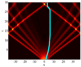
Figure 6.1: The figure shows the particle path $x_{1}(t)$ for a single Lagrangian fluid parcel obtained from $dx_{1}/dt=u_{1}(x_{1}(t),t)$, upon identifying the modified CH2 solutions $(u,\bar{\rho})$ of the 1D dam-break experiments studied in [23] with solutions $(u_{1},u_{2})$ of the EPDiff$(H^{1})$ equation (6.3) that are independent of the second coordinate, $x_{2}$, in a periodic domain. A fluid parcel initially offset to the right of center in $x_{1}$ accelerates gently to the right as the dam-break produces pulses that propagate away on the right side. Later, when the leading pulse returns leftward, the parcel is pushed suddenly back with considerably greater leftward acceleration and ends up nearly where it started. Its trajectory shows that the wave pulses propagate relative to the Lagrangian parcels, so they are not frozen into the fluid motion. However, the influence of the returning pulse shows that the Lagrangian motion is still strongly coupled to the waves. Figure courtesy of L. Ó Náraigh.

7 Conclusions/Discussion

Main results of the paper.

The stage was set in Section 2 for our discussions of the inverse scattering transform method for the two-component CH2 system. The CH2 Jost solutions were obtained in Section §3 and their asymptotic behavior was usedin Section §4 to reformulate the scattering problem as a Riemann-Hilbert problem (RHP) . By solving the RHP, multi - soliton solutions of CH2 were obtained as reflectionless potentials in Section §5. The soliton solutions of CH2 arising from the RHP expressed themselves in a parametric form corresponding to the Lagrangian representation of fluid dynamics. A slightly modified version of CH2 was found in Section §6 by considering translation invariant EPDiff solutions. The peakon solutions of EPDiff (diffeons) were shown graphically to interact with the Lagrangian fluid parcels by briefly sweeping them along the peakon trajectory. It remains an open problem, as to whether the modified version of CH2 in (6.1) – (6.2) is integrable.

Explicit outstanding problems.

The integrable systems properties CH2 discussed here open the door for further generalizations and applications, some of which have been presented in the paper and others that will be discussed elsewhere. In particular, CH2 is a member of a large family of integrable multi-component PDE based on the Schrödinger equation with an energy-dependent potential, as discussed in [20]. The numerical simulation of these PDE, and the formulation and analysis of their discrete integrable versions can be expected to attract considerable attention in future endeavors. One may expect the continuing interest in wave-breaking analysis for CH and CH2 to apply to the integrable PDE in the rest of the CH2 family, as well.

References

• [1] Acheson, D. J. Elementary Fluid Dynamics. Oxford University Press (Oxford, 1990).
• [2] Boutet deย Monvel A. and Shepelsky D.: Riemann-Hilbert approach for the CH equation on the line, C.R. Math. Acad. Sci. Paris 343 (2006) 627โ€“632.
• [3] Camassa, R. and Holm, D. D. An integrable shallow water equation with peaked solitons. Phys. Rev. Lett. 71, 1661โ€“1664 (1993)
• [4] Camassa, R., Holm, D. and Hyman, J. A new integrable shallow water equation. Adv. Appl. Mech. 31, (1994)
• [5] Chen M., Liu S.-Q. and Zhang Y. A two-component generalization of the Camassa-Holm equation and its solutions. Lett. Math. Phys. 75 (2006) 1โ€“15; nlin.SI/0501028.
• [6] Chen, R.M. and Liu Y. Wave Breaking and Global Existence for a Generalized Two-Component Camassa-Holm System, International Mathematics Research Notices, Article ID rnq118, 36 pages. (2010) doi10.1093/imrn/rnq118
• [7] Constantin, A. On the scattering problem for the CH equation. Proc. R. Soc. Lond. A 457, 953โ€“970 (2001)
• [8] Constantin A., Gerdjikov V. and Ivanov R. Inverse scattering transform for the CH equation, Inv. Problems 22 (2006), 2197โ€“2207; arXiv nlin/0603019v2 [nlin.SI].
• [9] Constantin, A. and Ivanov, R. Poisson structure and Action-Angle variables for the CH equation, Lett. Math. Phys. 76, 93โ€“108 (2006); nlin.SI/0602049
• [10] Constantin, A. and Ivanov, R.I. On an integrable two-component Camassa-Holm shallow water system. Phys. Lett. A 372 (2008), 7129โ€“7132.
• [11] Dai, H.-H. Model equations for nonlinear dispersive waves in a compressible Mooney-Rivlin rod. Acta Mech. 127, 193โ€“207 (1998)
• [12] Dullin H.ย R., Gottwald G.ย A. $\&$ Holm D.ย D. CH, Korteweg-de Vries-5 and other asymptotically equivalent equations for shallow water waves, Fluid Dynam. Res. 33 (2003), 73โ€“95.
• [13] Dullin H.ย R., Gottwald G.ย A. $\&$ Holm D.ย D. On asymptotically equivalent shallow water wave equations, Physica 190D (2004), 1โ€“14.
• [14] Escher J., Lechtenfeld O. and Yin, Z. Well-posedness and blow-up phenomena for the 2-component Camassa-Holm equation. Discrete Contin. Dyn. Syst. 19 (2007) 493โ€“513.
• [15] Falqui, G. On a Camassa-Holm type equation with two dependent variables. J. Phys. A 39 (2006), 327โ€“342.
• [16] Gui G. and Liu Y. On the global existence and wave-breaking criteria for the two-component Camassa-Holm system. J. Funct. Anal. 258 (2010) 4251โ€“4278.
• [17] Holm, D. D. Geometric Mechanics: II Rotating, Translating and Rolling, World Scientific Imperial College Press, Singapore, (2008), ISBN 978-1-84816-155-9.
• [18] Holm D.D. Peakons, in Encyclopedia of Mathematical Physics, eds. J.-P. Franรงoise, G.L. Naber and Tsou S.T. Oxford Elsevier, 2006 (ISBN 978-0-1251-2666-3), volume 4 pages 12โ€“20.
• [19] Holm D. D. and Ivanov R. I. Smooth and peaked solitons of the CH equation, J. Phys A Math. and Theor., Special issue on current trends in integrability and nonlinear phenomena, Expected online publication: October 2010.
• [20] Holm D. D. and Ivanov R. I. Multi-component generalizations of the CH equation: Geometrical Aspects, Peakons and Numerical Examples. In preparation, 2010.
• [21] Holm, D.ย D. and J.ย E. Marsden [2004], Momentum maps and measure-valued solutions (peakons, filaments and sheets) for the EPDiff equation, in The Breadth of Symplectic and Poisson Geometry, A Festshrift for Alan Weinstein, 203-235, Progr. Math., 232, J.ย E. Marsden and T.ย S. Ratiu, Editors, Birkhรคuser Boston, Boston, MA, 2004.
• [22] Holm, D. D., Marsden, J. E. and Ratiu, T. S. The Euler-Poincarรฉ equations and semidirect products with applications to continuum theories. Advances in Mathematics, 137(1):1โ€“81, 1998.
• [23] Holm D. D., ร“ Nรกraigh, L. and Tronci, C. Singular solutions of a modified two-component CH equation. Phys. Rev. E (3) 79 (2009), no. 1, 016601, 13 pp.
• [24] Holm D. D., Schmah, T. and Stoica, C. Geometric mechanics and symmetry. From finite to infinite dimensions. With solutions to selected exercises by D. C. P. Ellis. Oxford Texts in Applied and Engineering Mathematics, 12. Oxford University Press, Oxford, 2009.
• [25] Holm, D. D. and Tronci, C. Geodesic Vlasov equations and their integrable moment closures. J. Geom. Mech. 1 (2009) 181โ€“208.
• [26] Holm D. D., Trouvรฉ, A. and Younes, L. The Euler-Poincarรฉ theory of metamorphosis. Quart. Appl. Math. 67 (2009) 661โ€“685.
• [27] Henry, D. J. Infinite propagation speed for a two component Camassa-Holm equation. Discrete Contin. Dyn. Syst. Ser. B 12 (2009) 597โ€“606.
• [28] Ivanov R. I. Extended CH hierarchy and conserved quantities, Z. Naturforsch., 61a (2006) pp. 133โ€“138; nlin.SI/0601066.
• [29] Ivanov, R. I. Two-component integrable systems modelling shallow water waves: the constant vorticity case. Wave Motion 46 (2009), 389โ€“396.
• [30] Jaulent M. and Jean C. The inverse s๐‘ s-wave scattering problem for a class of potentials depending on energy. Comm. Math. Phys. 28 (1972) 177โ€“220.
• [31] Johnson, R. S. CH, Korteweg-de Vries and related models for water waves. J. Fluid. Mech. 457, 63โ€“82 (2002)
• [32] Johnson, R. S. The CH equation for water waves moving over a shear flow. Fluid Dynamics Research 33, 97โ€“111 (2003)
• [33] Kaup, D. J. A higher-order water wave equation and the method for solving it, Progr. Theor. Phys. 54 (1975) 396โ€“408.
• [34] Kuzโ€™min, P. A. On two-component generalizations of the Camassa-Holm equation. Mat. Zametki 81 (2007) 149โ€“152(Russian); translation in Math. Notes 81 (2007) 130โ€“134.
• [35] Liu S.-Q. and Zhang Y. Deformations of semisimple bi-Hamiltonian structures of hydrodynamic type, J. Geom. Phys. 54 (2005) 427โ€“53.
• [36] Novikov, S. P., Manakov, S. V., Pitaevsky, L. P. and Zakharov, V. E. Theory of solitons: the inverse scattering method. New York, Plenum, 1984
• [37] Olver, P. and Rosenau, P. Tri-Hamiltonian duality between solitons and solitary-wave solutions having compact support. Phys. Rev. E (3) 53 (1996) 1900โ€“1906.
• [38] Sattinger, D. H. and Szmigielski, J. A Riemann-Hilbert problem for an energy dependent Schrรถdinger operator. Inverse Problems 12 (1996) 1003โ€“1025.
• [39] Shabat A. and Martรญnez Alonso L. On the prolongation of a hierarchy of hydrodynamic chains. In New trends in integrability and partial solvability (ed. A.B. Shabat et al.), Proceedings of the NATO advanced research workshop, Cadiz, Spain 2002, NATO Science Series, Kluwer Academic Publishers, Dordrecht: 2004, pp. 263โ€“280.
• [40] Zhang, P. and Liu, Y. Stability of Solitary Waves and Wave-Breaking Phenomena for the Two-Component CH System, International Mathematics Research Notices 2010 (2010), No. 11, pp. 1981โ€“2021.