Weak localization in mesoscopic hole transport:
Berry phases and classical correlations

Abstract

We consider phase-coherent transport through ballistic and diffusive two-dimensional hole systems based on the Kohn-Luttinger Hamiltonian. We show that intrinsic heavy-hole light-hole coupling gives rise to clear-cut signatures of an associated Berry phase in the weak localization which renders the magneto-conductance profile distinctly different from electron transport. Non-universal classical correlations determine the strength of these Berry phase effects and the effective symmetry class, leading even to antilocalization-type features for circular quantum dots and Aharonov-Bohm rings in the absence of additional spin-orbit interaction. Our semiclassical predictions are quantitatively confirmed by numerical transport calculations.

As a genuine wave phenomenon, coherent backscattering, denoting enhanced backreflection of waves in complex media due to constructive interference of time-reversed paths, has been encountered in numerous systems. Its occurrence ranges from the observation of the infrared intensity reflected from Saturn’s rings B. W. Hapke and Smythe (1993) to light scattering in random media van Albada and Lagendijk (1985), from enhanced backscattering of seismic Larose et al. (2004) and acoustic Bayer and Niederdränk (1993) to atomic matter waves Hartung et al. (2008). In condensed matter, weak localization (WL) Abrahams et al. (1979); Altshuler et al., (1980), closely related to coherent backscattering, has been widely used as a diagnostic tool for probing phase coherence in conductors at low temperatures. Based on time-reversal symmetry (TRS), WL manifests itself as a characteristic dip in the average magneto conductivity at zero magnetic field $B$. The opposite phenomenon, a peak at $B\!=\!0$, is usually interpreted as weak antilocalization (WAL) due to spin-orbit interaction (SOI) S. Hikami and Nagaoka (1980).

In this Letter we show that the average magneto conductance of mesoscopic systems built from two-dimensional hole gases (2DHG) distinctly deviates from the corresponding WL transmission dip profiles of their n-doped counterparts. In particular, ballistic hole conductors such as circular quantum dots and Aharonov-Bohm (AB) rings, can exhibit a conductance peak at $B\!=\!0$, even in the absence of SOI Winkler (2003) due to structure (SIA) or bulk inversion (BIA) asymmetry. We trace this back to effective TRS breaking of hole systems at $B\!=\!0$.

Recently, various magnetotransport measurements on such high-mobility 2DHG have been performed for GaAs bulk samples McPhail et al., (2004), quasi-ballistic cavities Faniel et al. (2007) and AB rings Yau et al. (2002); Grbić et al. (2007). However, we are not aware of corresponding theoretical approaches for ballistic 2DHG nanoconductors (except for 1d models Jääskeläinen and Zülicke (2010)), despite the huge number of theory works on ballistic electron transport Ferry and Goodnick (1997); Beenakker (1997). Here we treat 2DHG-based ballistic and diffusive mesoscopic structures on the level of the 4-band Kohn-Luttinger Hamiltonian Luttinger and Kohn (1955). By devising a semiclassical approach for ballistic, coupled heavy-hole (HH) light-hole (LH) dynamics we can associate the anomalous WL features directly with Berry phases Berry (1984) in the Kohn-Luttinger model Chang and Niu (1996); Haldane (2004); Chang and Niu (2008) (that have proven relevant e.g. for the spin Hall effect Murakami et al. (2003)). We show that the strength of the related effective ’Berry field’, giving rise to effective TRS breaking and a splitting of the WL dip, is determined by a classical correlation between enclosed areas and reflection angles of interfering hole trajectories relevant for WL. This system-dependent geometrical correlation is not amenable to existing random matrix approaches for chaotic conductors Beenakker (1997). We confirm our semiclassical results by numerical quantum transport calculations and further discuss the additional effect of SOI.

Hamiltonian and band structure.– To describe the 2DHG we represent the Kohn-Luttinger Hamiltonian Luttinger and Kohn (1955) for the two uppermost valence bands of a semiconductor in terms of an eigenmode expansion for an infinite square well of width $a$ modelling the vertical confinement. Employing Löwdin partitioning Löwdin (1951) we construct an effective Hamiltonian based on the relevant, lowest subband in $z$-direction com . The resulting $4\!\times\!4$-Luttinger Hamiltonian for a quasi 2DHG then describes coupled HH and LH states with spin projection $\pm 3/2$, and $\pm 1/2$, respectively. Without SOI due to SIA or BIA, the 2DHG Hamiltonian splits into decoupled blocks:

$$\hat{\mathcal{H}}_{\mathrm{2D}}=\begin{pmatrix}\hat{P}&\hat{T}&&\\ \hat{T}^{\dagger}&\hat{Q}&&\\ &&\hat{Q}&\hat{T}\\ &&\hat{T}^{\dagger}&\hat{P}\end{pmatrix}=\begin{pmatrix}\hat{\mathcal{H}}_{\mathrm{U}}&\\ &\hat{\mathcal{H}}_{\mathrm{L}}\\ \end{pmatrix}\text{\hskip 8.5359pt},\,\begin{matrix}\mathrm{HH}\Uparrow\\ \mathrm{LH}\downarrow\\ \mathrm{LH}\uparrow\\ \mathrm{HH}\Downarrow\end{matrix}$$ (1)

with the upper and lower blocks composed of Broido and Sham (1985)

$$\hat{P} = -\frac{\hbar^{2}}{2m_{0}}\left[(\gamma_{1}+\gamma_{2})\hat{k}_{\|}^{2}+(\gamma_{1}-2\gamma_{2})\langle\hat{k}_{z}^{2}\rangle\right]\text{,}$$ (2a)

$$\hat{Q} = -\frac{\hbar^{2}}{2m_{0}}\left[(\gamma_{1}-\gamma_{2})\hat{k}_{\|}^{2}+(\gamma_{1}+2\gamma_{2})\langle\hat{k}_{z}^{2}\rangle\right]\text{,}$$ (2b)

$$\hat{T} = -\sqrt{3}\frac{\hbar^{2}}{2m_{0}}\left[\gamma_{2}(\hat{k}_{x}^{2}-\hat{k}_{y}^{2})+2\mathrm{i}\gamma_{3}\hat{k}_{x}\hat{k}_{y}\right]\text{.}$$ (2c)

Here, $\hat{\bf k}=(\hat{k}_{x},\hat{k}_{y},\hat{k}_{z})$ is the wave vector with projection $\hat{k}_{\|}$ onto the $xy$-plane of the 2DHG and $\langle\hat{k}_{z}^{2}\rangle\!=\!(\pi/a)^{2}$ is the expectation value of $k_{z}$ for the lowest subband. Below we use the axial approximation, $\bar{\gamma}\!=\!\gamma_{2}\!=\!\gamma_{3}$, for the parameters in $\hat{T}$ that couple HH and LH states.

Due to the 2D confinement the HH-LH bulk degeneracy is lifted which will play an important role for the WL analysis below. To this end we will calculate the two-terminal Landauer conductance

$$G=\frac{e^{2}}{h}T=\frac{e^{2}}{h}\sum^{N}_{n,m}\sum_{\sigma,\sigma^{\prime}}|t_{m,\sigma^{\prime};n,\sigma}|^{2}$$ (3)

with the transmission amplitudes $t_{m,\sigma^{\prime};n,\sigma}$ given by the Fisher-Lee relations Fisher and Lee (1981). The indices $m$ and $n$ label $N$ transverse modes in the leads, and $\sigma\in\{\mathrm{U},\mathrm{L}\}$ with $\mathrm{U}\in\{{\mathrm{HH}\Uparrow,\mathrm{LH}\downarrow}\}$ and $\mathrm{L}\in\{\mathrm{HH}\Downarrow,\mathrm{LH}\uparrow\}$ denotes the HH and LH modes. The Hamiltonian (1) with blocks obeying $\hat{\mathcal{H}}_{\mathrm{U}}(B)\!=\!\hat{\mathcal{H}}^{\dagger}_{\mathrm{L}}(-B)$ (neglecting Zeeman spin splitting) allows us to separately define related total transmissions, $T_{\mathrm{U}},T_{\mathrm{L}}$, with $T\!=\!T_{\mathrm{U}}\!+\!T_{\mathrm{L}}$ fulfilling $T_{\mathrm{U}}(B)\!=\!T_{\mathrm{L}}(-B)$.

Depending on the position of the Fermi level $E_{\rm F}$ we distinguish the case where HH and LH states are both occupied (considered at the end of this Letter) from the case where $E_{\rm F}$ is close to the band gap such that only HH states contribute to transport. We first study the latter case with focus on effects from the HH-LH coupling.

HH-LH coupling and Berry phase.- For ballistic mesoscopic systems of linear size $L$ in the regime $kL\!\gg\!1$ we will generalize the semiclassical approaches Baranger et al. (1993a); Richter and Sieber (2002) to the Landauer conductance from electron systems with a parabolic dispersion to the p-doped case with more complex band topology. The HH-LH coupling enters into the semiclassical formalism as an additional phase that is accumulated during each reflection of a HH wave packet at a smooth boundary potential (the hard wall case is considered below). Such a reflection can be described as an adiabatic transition in momentum space leading to a geometric phase acquired along a given path Chang and Niu (1996); Haldane (2004):

$$\Gamma_{\sigma}\!=\!\int\!\mathcal{A}_{\sigma}(\textbf{\em k})d\textbf{\em k}\quad;\quad\mathcal{A}_{\sigma}(\textbf{\em k})\!=\!-\mathrm{i}\langle\psi_{\sigma}(\textbf{\em k})|\nabla_{k}\psi_{\sigma}(\textbf{\em k})\rangle\,.$$ (4)

Using for $\psi_{\sigma}(\textbf{\em k})$ the free solutions of Hamiltonian (1) we find after diagonalization for the vector potential

$$\mathcal{A}_{\mathrm{HH}\Uparrow}(\textbf{\em k})=-\mathcal{A}_{\mathrm{HH}\Downarrow}(\textbf{\em k})=3\frac{\xi^{\rm Berry}(k)}{k^{2}}\begin{pmatrix}k_{y}\\ -k_{x}\end{pmatrix}$$ (5)

and $\mathcal{A}_{\mathrm{LH}\downarrow}(\textbf{\em k})=\mathcal{-}A_{\mathrm{LH}\uparrow}(\textbf{\em k})=-[(3\xi+2)/3\xi]\mathcal{A}_{\mathrm{HH}\Uparrow}(\textbf{\em k})$ with $\xi^{\rm Berry}(k)\!\simeq\!-\tfrac{1}{8}(\tfrac{ka}{\pi})^{4}$, to leading order in $ka/\pi$. The Berry phase for a single reflection at a smooth boundary is then

$$\Gamma_{\mathrm{HH}\Uparrow}^{\rm Berry}(\varphi)=-\Gamma_{\mathrm{HH}\Downarrow}^{\rm Berry}(\varphi)=\xi^{\rm Berry}\sin\varphi(2-\cos\varphi)\,,$$ (6)

where $\varphi$ denotes the change in momentum direction.

For a specular reflection at a hard-wall (hw) confinement a corresponding phase shift is obtained by requiring that the propagating HH and the evanescent LH part of the reflected wave both must vanish at the boundary:

$$\Gamma_{\mathrm{HH}\Uparrow}^{\rm hw}(\varphi) \!=\! \frac{1}{\mathrm{i}}\ln\frac{2-\xi^{\rm hw}e^{-2\mathrm{i}\,\varphi}}{|2-\xi^{\rm hw}e^{-2\mathrm{i}\,\varphi}|}\stackrel{{\scriptstyle\xi^{\rm hw}\ll 1}}{{\simeq}}\xi^{\rm hw}\sin 2\varphi\,,$$ (7)

with $$\xi^{\rm hw}(k)\simeq-\frac{\gamma_{1}+\bar{\gamma}}{4\bar{\gamma}}\left(\frac{ka}{\pi}\right)^{2}\,.$$ (8)

Average magneto conductance.- A semiclassical approach proves convenient to incorporate these additional (Berry) phases into a theory of WL. For a (chaotic) ballistic quantum dot the known semiclassical amplitude Baranger et al. (1993a) for electron transmission from channel $n$ to $m$ is generalized to $t_{m,\mathrm{HH}\Uparrow;n,\mathrm{HH}\Uparrow}\!\simeq\!\sum_{\gamma}C_{\gamma}K_{\gamma}\exp(\tfrac{\mathrm{i}}{\hbar}\mathcal{S}_{\gamma})$, in terms of a sum over lead-connecting classical paths $\gamma$ with classical action $\mathcal{S}_{\gamma}$, weight $C_{\gamma}$ (including the Maslov index) and an additional factor $K_{\gamma}\!=\!\exp[\mathrm{i}\sum_{j=1}^{n_{b}}\Gamma_{\mathrm{HH}\Uparrow}(\varphi_{j})]$ accounting for the accumulated phases (6) or (7) after $n_{b}$ successive reflections. In view of Eq. (3) the total semiclassical transmission probability for HH$\Uparrow$ states reads

$$T_{\rm U}\simeq\sum_{n,m}\sum_{\gamma\gamma^{\prime}}K_{\gamma}K^{*}_{\gamma^{\prime}}C_{\gamma}C^{*}_{\gamma^{\prime}}\mathrm{e}^{\tfrac{\mathrm{i}}{\hbar}(\mathcal{S}_{\gamma}-\mathcal{S}_{\gamma^{\prime}})}\mathrm{.}$$ (9)

The diagonal contribution, $\gamma\!=\!\gamma^{\prime}$, correctly yields the classical transmission since $K_{\gamma}K^{*}_{\gamma}\!=\!1$. WL contributions arise (after averaging) from off-diagonal pairs of long, classically correlated paths $\gamma\!\neq\!\gamma^{\prime}$ with small action difference ($\mathcal{S}_{\gamma}\!-\!\mathcal{S}_{\gamma^{\prime}}\!\sim\!\hbar$), where $\gamma$ forms a loop and $\gamma^{\prime}$ follows the loop in opposite direction, while it coincides with $\gamma$ for the rest of the trajectory Richter and Sieber (2002). Due to the time-reversed traversal of the loop the two paths acquire, in the presence of a magnetic field $B$, an additional action difference $(\mathcal{S}_{\gamma}-\mathcal{S}_{\gamma^{\prime}})/\hbar\!=\!4\pi AB/\Phi_{0}$, where $A$ is the enclosed (loop) area and $\Phi_{0}$ the flux quantum. Moreover, during the loop $\gamma$ and $\gamma^{\prime}$ have opposite reflections, $\varphi_{j}\!=\!-\varphi_{j}^{\prime}$, and hence

$$K_{\gamma}K^{*}_{\gamma^{\prime}}=\exp[2\mathrm{i}\sum_{j=1}^{n_{b}}\ \Gamma_{\mathrm{HH}\Uparrow}(\varphi_{j})\ ]\,.$$ (10)

For chaotic dynamics in a cavity where the escape length $L_{\mathrm{esc}}$ is much larger than the average distance $L_{b}$ between consecutive bounces we can introduce probability distributions for the areas $A$ and the phases $\sum_{j=1}^{n_{b}}\Gamma_{\mathrm{HH}\Uparrow}(\varphi_{j})$. Our classical simulations for both the smooth and the hw case revealed Krueckl2010 that the probability distributions of $\sum_{j=1}^{n_{b}}\Gamma_{\mathrm{HH}\Uparrow}(\varphi_{j})$ coincide very well (for $n_{b}\!>\!5$ and $\xi\!<\!1$) with the distribution $\tilde{\xi}\sum_{j=1}^{n_{b}}\varphi_{j}$ with a renormalized HH-LH coupling $\tilde{\xi}^{\rm Berry}\simeq 0.6\xi^{\rm Berry}$ and $\tilde{\xi}^{\rm hw}\simeq 0.2\xi^{\rm hw}$. This allows us to treat both cases on equal footing by replacing Eq. (10) through $K_{\gamma}K^{*}_{\gamma^{\prime}}=e^{2\mathrm{i}\ \tilde{\xi}\alpha}$ with $\alpha\!=\!\sum^{n_{b}}_{j=1}\varphi_{j}$.

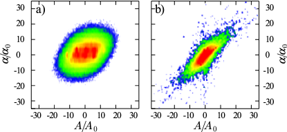
Figure 1: (Color online) Probability distributions to find an orbit with enclosed area $A$ and accumulated angle $\alpha$ for (a) a chaotic cavity (inset Fig. 3(a)) and (b) a disc (inset Fig. 3(b)). (Red (central) regions correspond to high probability).

Generalizing the semiclassical approaches for electron Baranger et al. (1993a); Richter and Sieber (2002) to HH $\Uparrow(\Downarrow)$ transport the WL correction can then be expressed as an integral over trajectory lengths,

$$\delta T_{\rm U(L)}=\frac{\delta T^{(0)}}{L_{\mathrm{esc}}}\int_{0}^{\infty}\mathrm{e}^{-L/L_{\mathrm{esc}}}\mathcal{M}(L;B,\mp\tilde{\xi})\leavevmode\nobreak\ dL\,.$$ (11)

Here $\delta T^{(0)}$ is the WL correction for $B\!=\!0,\tilde{\xi}\!=\!0$ ($\delta T^{(0)}\!=\!-1/(4\!-\!2/N)$ for a chaotic electronic conductor Beenakker (1997)), and

$$\mathcal{M}(L;B,\tilde{\xi})\!=\!\int_{-\infty}^{\infty}\!\!\!dA\int_{-\infty}^{\infty}\!\!\!d\alpha P_{L}(A,\alpha)\\ e^{2\pi\mathrm{i}[\tilde{\xi}\alpha/\pi+2AB/\Phi_{0}]}\,,$$ (12)

where $P_{L}(A,\alpha)$ is the joint probability distribution for the accumulated areas and angles. While both parameters follow Gaussian distributions, we stress that there exist non-universal correlations between $A$ and $\alpha$ reflecting the geometry of the quantum dot. When plotting $P_{L}(A,\alpha)$ these correlations show up as deviations from a circular symmetry, as illustrated in Fig. 1(a) showing classical simulations for a chaotic cavity (inset Fig. 3(a)).

The central limit theorem implies a two-dimensional multivariate normal distribution,

$$P_{L}(A,\alpha)\!=\!\frac{1}{2\pi\sigma}\!\exp\!\left[-\frac{(A/A_{0})^{2}\!+\!(\alpha/\alpha_{0})^{2}\!-\!2\rho A\alpha/(A_{0}\alpha_{0})}{2(1-\rho^{2})L/L_{b}}\right]$$ (13)

with $\!\sigma\!\!=\!\!A_{0}\alpha_{0}\!\sqrt{(1\!-\!\rho^{2})L/L_{b}}$. Correlations are encoded in $\rho$ ranging from 0 to $\!\pm 1$. Assuming ergodicity we obtain for the variances of the angle $\alpha_{0}^{2}\!=\!4(\pi\!-\!2)$, area $A_{0}^{2}\!\simeq\!\tfrac{2}{15}[L_{b}^{2}\!+\!{\rm var}(L_{b})]^{2}$ and covariance $\rho A_{0}\alpha_{0}\!=\!L_{b}^{2}(\tfrac{\pi}{4}\!-\!\tfrac{1}{3})$ Krueckl2010 . This leads to the geometry-dependent $\rho\!\simeq\!0.58/[1\!+\!{\rm var}(L_{b})/L_{b}^{2}]$, i.e., $\rho\!<\!0.58$ for a chaotic system. ($\rho\approx 0.5$ for the cavity in Fig. 3(a).) The correlations can be stronger in non-chaotic systems and are pronounced for a disk (inset Fig. 3(b)) as we see in Fig. 1(b). (We find $\rho\!\approx\!0.8$.)

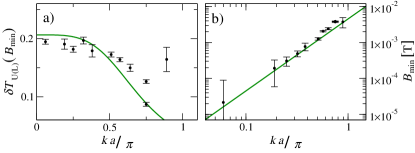
Figure 2: (Color online) Dependence of (a) the depth $\delta T_{U(L)}(B_{\rm min})$ and (b) the position $B_{\rm min}$ of the magneto transmission weak localization dip on $ka$ (governing the effective HH-LH coupling, see Eq. (8)) for HH transport through a chaotic quantum dot (inset Fig. 3(a)). Numerical quantum results (symbols) are compared to the semiclassical predictions (15,16) ((green) lines) for $\gamma_{1}\!=\!6.85$, $\bar{\gamma}\!=\!2.5$ (for GaAs).

Using Eqs. (12,13) we get from Eq. (11) semiclassically a Lorentzian WL dip magneto conductance profile

$$\delta T_{\rm U(L)}(B)=\frac{\beta\delta T^{(0)}}{1\!+\![2\pi\sqrt{2\beta}A_{0}(B\!\mp\!B_{\mathrm{Berry}})/\Phi_{0})]^{2}L_{\mathrm{esc}}/L_{b}}$$ (14)

with a depth $\delta T_{\rm U(L)}(B_{\rm min})\!=\!\beta\delta T^{(0)}$ with

$$\beta=[1+2\alpha_{0}^{2}(1-\rho^{2})\tilde{\xi}^{2}L_{\mathrm{esc}}/L_{b}]^{-1}\,.$$ (15)

As a main result, the WL dip is shifted by the Berry field

$$B_{\mathrm{Berry}}=\rho\ \tilde{\xi}\ \frac{\alpha_{0}\Phi_{0}}{2\pi A_{0}}\,,$$ (16)

which relies on both, quantum HH-LH coupling $\tilde{\xi}$ and finite classical $A$-$\alpha$ correlations $\rho$.

In Fig. 2(a,b) we compare our predictions (15,16) for the dip depth, $\delta T_{U}(B_{\rm min})\!=\!-\beta/(4\!-\!2/N)$, and displacement, $B_{\rm Berry}$, with numerical recursive Green function calculations Wimmer2009 of these quantities for a chaotic quantum dot (inset Fig. 3(a)) for different HH-LH couplings by tuning the vertical confinement $a$. The quantum results (symbols) show quantitative agreement with the semiclassical curves (green lines), which are entirely based on the classical parameters $A_{0},\alpha_{0}$ and $\rho$.

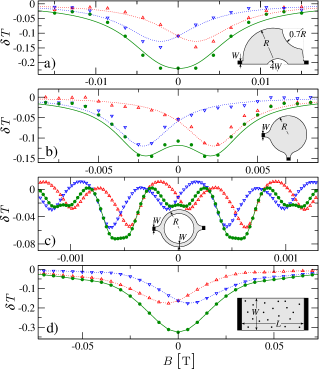
Figure 3: (Color online) HH-LH coupling-induced Berry phase effects on weak localization in various mesoscopic hole gases. The WL correction $\delta T$ is shown for a ballistic chaotic cavity (a), disc (b), AB ring (c) and a diffusive strip (d). Red ($\triangle$) and blue ($\nabla$) triangles denote quantum mechanical transmissions $\delta T_{\rm U}(B),\delta T_{\rm L}(B)$ adding up to the full $\delta T(B)$ (green bullets, see text below Eq. (3)). The red and blue dotted curves in a) and b) show our semiclassical results (14) with the horizontal displacements given by the Berry field (16) reflecting geometrical correlations (based on the calculated classical quantities $A_{0}\simeq 12200(56129)\mbox{nm}^{2}$, $\alpha_{0}\simeq 1.92(5.89)$, $\rho\!\simeq\!-0.5(-0.8)$ in a), (b))). In c), d) the lines are guides to the eye of the quantum results. Parameters used: $\gamma_{1}\!=\!6.85$, $\bar{\gamma}\!=\!2.5$, $ka/\pi\!=\!0.64$; a), b), c): 5 and d) 15 open modes per subblock. Geometries (lengths in units of nm): a): $R\!=\!350,W\!=\!40$, b): $R\!=\!200,W\!=\!40$, c): $R\!=\!800,W\!=\!40$, d): $L\!=\!2000,W\!=\!120$. Averages taken over $\sim 2000$ energies and geometries (a-c) and $\sim 1000$ disorder configurations (d).

Finally, we analyze in the central Fig. 3 the effect of the geometrical correlation $\rho$ on WL in different representative mesoscopic systems for fixed, realistic HH-LH coupling. Panel (a) depicts the WL transmission profile of a chaotic cavity. Our semiclassical results (without free parameters) show remarkable agreement with the quantum calculations. The nonzero $\rho\approx 0.5$ gives rise to a splitting of the $T_{U}$ and $T_{L}$ traces by $2B_{\rm Berry}$ leading to a flattened WL dip for $T=T_{\rm U}+T_{\rm L}$ compared to the Lorentzian WL profile for electrons. Panel (b) shows results for the circular dot with larger correlation ($\rho\approx 0.8$). Accordingly, the Berry field is stronger leading to an WAL-type overall profile. Correspondingly, we find in the averaged transmission of AB-rings (panel (c)) distinct additional features at $B\!=\!0$ Zulicke-comment absent in electron transport.

We close with several remarks:

(i) Corresponding transport calculations for dots with smooth confinement yield a $ka$ scaling of $B_{\rm Berry}$ close to the quartic behavior predicted by $\xi^{\rm Berry}$ from Eq. (5).

(ii) The correlation mechanism is not restricted to ballistic but also relevant in diffusive systems, as illustrated in Fig. 3(d), leading to broadening and deviations of the WL profile from that of a digamma function for electrons.

(iii) If HH and LH states are both occupied and contribute to transport, our quantum calculations show a vanishing WL correction both for diffusive and chaotic ballistic conductors Krueckl2010 which, as far as we know, has not been reported before. Although the full Hamiltonian (1) obeys TRS for $B\!=\!0$, transport is governed by the individual subblocks $\hat{\mathcal{H}}_{\mathrm{U}},\hat{\mathcal{H}}_{\mathrm{L}}$ that do not possess TRS, and hence WL is suppressed in a 2DHG with strong coupling between occupied HH and LH states. It is notable that this kind of effective TRS breaking, recently discussed in the context of graphene and topological insulators Bernevig2006 , is already present in the well-established system of a 2DHG. Interestingly, if only HH states are occupied, TRS breaking in each subblock can be traced back to the Berry field (16), i.e. system-specific classical correlations determine the degree of TRS breaking, and hence the mere knowledge of the overall universality class is insufficient.

(iv) SOI terms due to SIA and BIA couple the subblocks, eventually restore TRS and give rise to WAL effects on top of the mechanisms illustrated in Fig. 3; we checked this numerically for BIA for the diffusive and ballistic case Krueckl2010 . Hence in 2DHG-based AB measurements such as Yau et al. (2002); Grbić et al. (2007) presumably both SOI and HH-LH coupling-induced phases affect the AB signal. The latter mechanism should be more clearly observable in systems with reduced SOI such as WL studies in Si Kuntsevich2007 . Moreover these WAL effects might also be visible in p-doped ferromagnetic semiconductors such as GaMnAs Neu07 . From our analysis we expect to observe equivalent WL effects also in other 2D systems where the band structure gives rise to geometric phases. Promising candidates are e.g. HgTe-based quantum wells with a tunable band topology Bernevig2006 that is directly related to the Berry connection Fu2006 .