Second Moment Method on k-SAT: a General Framework

Abstract

We give a general framework implementing the Second Moment Method on k-SAT and discuss the conditions making the Second Moment Method work in this framework. As applications, we make the Second Moment Method work on boolean solutions and implicants. We extend this to the distributional model of k-SAT.

1 Introduction to the Second Moment Method

Just as the First Moment Method is a way to upper-bound the threshold of k-SAT, so is the Second Moment Method a way to lower-bound it. After a brief technical introduction to the Second Moment Method in section 1.1, we present in section 1.2 a survey of the early attempts to lower-bound the threshold of 3-SAT through the Second Moment Method. As in the First Moment Method, the general idea is to count special kinds of solutions. However, the selection of solutions is not the same as in the First Moment Method:

1. in the First Moment Method, we considered random variables $X$ such that satisfiability implies $X\geq 1$; setting $X$ to be the number of solutions yields an upper bound of $5.191$ for the threshold of 3-SAT; and we tried to select the least solutions;

2. in the Second Moment Method, we shall consider random variables $X$ such that unsatisfiability implies $X=0$ (see section 1.1); setting $X$ to be the number of solutions yields a lower bound of $0$ for the threshold of 3-SAT (see section 1.2.1); here the criterion to select solutions is quite different: we are interested in subsets of solutions having low variance.

In a breakthrough paper, Achlioptas & Peres - 2004 [2] succeeded with the Second Moment Method on k-SAT, establishing a lower bound of $2.68$ for 3-SAT and an asymptotically tight lower bound of $2^{k}\ln 2-O\left(k\right)$ for k-SAT. It turns out that the currently best lower bound of the 3-SAT threshold ($3.52$) was obtained by another way: analyzing algorithms finding solutions with high probability, cf. Kaporis, Kirousis & Lalas [8] and Hajiaghayi & Sorkin [6].

The purpose of the next chapters is to make the most of the Second Moment Method on k-SAT. To do so we take a different approach from Achlioptas & Peres’. In our framework we select solutions according to the fraction of variables assigned $1$ and the fractions of the different types of clauses (i.e. the number of true literals occurrences in the clauses). This framework is general enough to include boolean solutions, implicants etc. However, tuning our parameters the best way we could, we got numerical evidence that we could not obtain better lower bounds than $2.83$.

The stumbling block we recurrently encountered is what we call the independence point. It corresponds to the couples of independent solutions in the subset of selected solutions. Even though solutions are independent, the proportion of literals occurrences having a certain truth value may not be independent between solutions. We got numerical evidence that the Second Moment Method does not work if truth values of literals occurrences are not independent. On the other hand, when they are independent, we give a necessary condition for the Second Moment Method to work, taking into account just the exponential equivalent of the second moment at this point. This condition tells us that we must select solutions having equal true and false surfaces (the surface is just the total number of literals occurrences), which is very artificial with respect to what we can observe with SATLab [7]. Using this condition, we could make the Second Moment Method work numerically; however, since the lower bounds we get ($2.83$) are far below the currently best lower bound ($3.52$), we do not give a rigorous (and tedious) proof of our lower bounds (to do so, the exponential equivalent would not be enough, and calculations would become quite involved).

The very restrictive conditions we encountered to make the Second Moment Method work may be due to some weaknesses of our framework. We do not claim that the Second Moment Method is doomed to perpetual failure on k-SAT. We only hope to shed a small ray of light onto it. This work is very fresh, still in progress, and has not been published.

In section 2 we present a general framework implementing the Second Moment Method on random k-SAT under various settings (distributions of signs, implicants…). Section 3 is dedicated to a variation of the framework presented in section 2 for the needs of distributional models.

1.1 How the Second Moment Method Is Supposed to Work

Let us recall how the Second Moment Method is supposed to work: given an event $A$, we want to show that $\mathrm{Pr}\left(A\right)$ tends to $1$ but we don’t have access to $\mathrm{Pr}\left(A\right)$. Instead we use the first and the second moments of a non-negative random variable $X$ such that $\mathrm{Pr}\left(A\right)\geq\mathrm{Pr}\left(X>0\right)$, i.e. $X$ must be $0$ when $A$ does not hold. For our problem 3-SAT, $A$ is the event “a formula is satisfiable”. The simplest choice for $X$ is of course the number of solutions.

1. The first thing to notice is that if we show that $\mathrm{Pr}\left(A\right)$ is lower-bounded by a positive constant, then it tends to $1$. Why? Because Friedgut & Bourgain’s theorem [5] established a sharp threshold for random k-SAT;

2. In order to prove that $\mathrm{Pr}\left(X>0\right)$ is bounded away from zero, we use the following classical identity:

   $$\mathrm{Pr}\left(X>0\right) \geq \frac{\left(\mathrm{E}X\right)^{2}}{\mathrm{E}X^{2}}\enskip.$$ (1)

   To prove it, use the fact that $\mathrm{E}X=\mathrm{E}\left(X\boldsymbol{1}_{X>0}\right)$ since $X\geq 0$, and apply the Cauchy-Schwartz inequality to it: $\left(\mathrm{E}X\right)^{2}\leq\mathrm{E}X^{2}\mathrm{E}\boldsymbol{1}_{X>0}^{2}$. So in particular note that

   $$\frac{\left(\mathrm{E}X\right)^{2}}{\mathrm{E}X^{2}} \leq 1\enskip.$$ (2)

Just as the first moment is fairly easy to compute, so is the second moment. Let $X$ be the number of assignments having some property $\mathcal{P}$ ($\mathcal{P}$ might be “be a solution” or “be a black and red polka-dot solution”):

$$\mathrm{E}\left(X^{2}\right) = \mathrm{E}\left(\left(\sum_{\sigma\mathrm{\,assignment}}\boldsymbol{1}_{\sigma\in\mathcal{P}}\right)^{2}\right)$$

$$= \mathrm{E}\left(\sum_{\sigma,\tau\mathrm{\,assignments}}\boldsymbol{1}_{\sigma\in\mathcal{P}}\boldsymbol{1}_{\tau\in\mathcal{P}}\right)$$

$$= \sum_{\sigma,\tau\mathrm{\,assignments}}\mathrm{E}\boldsymbol{1}_{\sigma\in\mathcal{P}\land\tau\in\mathcal{P}}$$

$$= \sum_{\sigma,\tau\mathrm{\,assignments}}\mathrm{Pr}\left(\sigma\in\mathcal{P}\land\tau\in\mathcal{P}\right)\enskip.$$

In the case of satisfiability however, we are going to see that the Second Moment Method is much more difficult to implement than the First Moment Method. The reason is that in general $\mathrm{E}X^{2}$ tends to be exponentially greater than $\left(\mathrm{E}X\right)^{2}$, so equation 1 just says that $\mathrm{Pr}\left(X>0\right)\geq 0$, which is not very informative… Thus the challenge is to find out a set of solutions having low variance.

1.2 Use of the Second Moment Method for Lower-Bounding the Threshold of k-SAT

In this section we make a survey of different applications of the Second Moment Method to lower-bound the threshold of random k-SAT. The model considered here is uniform random drawing of k-SAT.

1.2.1 Second Moment of Solutions

Here is a perfect example of the failure of the Second Moment Method. Namely the lower bound obtained by the Second Moment Method of solutions is $c=0$. If $X$ is just the number of solutions, then $\mathrm{E}X=2^{n}\left(1-\frac{1}{2^{k}}\right)^{cn}$. So let us now compute the second moment.

To do so we need an extra parameter $\mu$, representing the proportion of variables changing values between two solutions.

1. total number of couples of assignments:

   1. choose the value of variables assigned $0$ or $1$ in the first assignment: $2^{n}$;

   2. choose the subset of variables assigned different values in both assignments: ${n\choose\mu n}$;

2. probability for a couple of assignments to be a couple of solutions: as noted by Achlioptas & Peres [2], it is easier to compute the probability that a clause breaks two given assignments, since it is $\left(\frac{1-\mu}{2}\right)^{k}$. Using then the fact that $\mathrm{Pr}\left(A\cap B\right)=1-\mathrm{Pr}\left(\overline{A}\cup\overline{B}\right)=1-\mathrm{Pr}\left(\overline{A}\right)-\mathrm{Pr}\left(\overline{B}\right)+\mathrm{Pr}\left(\overline{A}\cap\overline{B}\right)$, it follows that the probability for a clause not to break any of both assignments is $g\left(\mu\right)=1-\frac{2}{2^{k}}+\left(\frac{1-\mu}{2}\right)^{k}$.

Thus the second moment is:

$$\mathrm{E}X^{2} = 2^{n}\sum_{\begin{subarray}{c}0\leq\mu\leq 1\\ \mu n\in\boldsymbol{N}\end{subarray}}{n\choose\mu n}g\left(\mu\right)^{cn}\enskip.$$

Let us look at the exponential equivalent of this quantity:

$$\mathrm{E}X^{2}\asymp\max_{0\leq\mu\leq 1}\left(\frac{2}{\mu^{\mu}\left(1-\mu\right)^{\mu}}g\left(\mu\right)^{c}\right)^{n}\enskip.$$

As explained by Achlioptas & Peres [2], it turns out that when $\mu=\frac{1}{2}$, this is precisely $\left(\mathrm{E}X\right)^{2}$. Now the function $\mu\mapsto\frac{1}{\mu^{\mu}\left(1-\mu\right)^{1-\mu}}$ has its maximum at $\mu=\frac{1}{2}$, whereas $g\left(\mu\right)$ is strictly decreasing over $\left(0,1\right)$. Consequently, at any positive ratio $c$, the maximum of $\frac{2}{\mu^{\mu}\left(1-\mu\right)^{\mu}}g\left(\mu\right)^{c}$ occurs at $\mu<\frac{1}{2}$ and $\mathrm{E}X^{2}$ is exponentially greater than $\left(\mathrm{E}X\right)^{2}$. So $\frac{\left(\mathrm{E}X\right)^{2}}{\mathrm{E}X^{2}}$ tends to zero, and we only get that $\mathrm{Pr}\left(X>0\right)\geq 0$…

1.2.2 Balancing True and False Surfaces

Achlioptas & Moore - 2002 [1] noticed that $g\left(\mu\right)$ is locally maximal at $\mu=\frac{1}{2}$ in k-NAE-SAT because in this problem $g\left(\mu\right)=1-\frac{4}{2^{k}}+\frac{1}{2^{k}}\left(\left(1-\mu\right)^{k}+\mu^{k}\right)$ is symmetric in $\mu$. We recall that in NAE-SAT, when an assignment is a solution, then the opposite assignment is a solution as well. Thus this problem contains some symmetry. Using this remark, Achlioptas & Moore were able to establish a tight lower bound on the k-NAE-SAT threshold. And since a NAE-SAT solution is a solution of standard SAT, they got the following lower bound of the k-SAT threshold: $2^{k-1}\ln 2-O\left(1\right)$.

Achlioptas & Peres - 2004 [2] put some weights onto the solutions of standard SAT and got a lower bound of $2^{k}\ln 2-O\left(k\right)$. (thus almost matching the asymptotic upper bound of $2^{k}\ln 2$). The weights they put are of the form $\lambda^{\mathrm{true\,surface}}\boldsymbol{1}_{\mathrm{SAT}}$, where the true surface is the number of occurrences of true literals under the solution. Assignments which are not solutions must be discarded because the Second Moment Method requires to count $0$ when there is no solution, as explained in section 1.1. In the particular case of 3-SAT they got a lower bound of $2.54$ (and even $2.68$ with a refinement).

We are going to implement the Second Moment Method without any weights; so how shall we control the balance of true and false surfaces? Our control parameters will be $\beta_{t}$, the fraction of clauses having $t$ true literals. Then the true surface will be $\beta_{1}+2\beta_{2}+3\beta_{3}$ and the false surface will be $2\beta_{1}+\beta_{2}$. With this parameters we are able to make the Second Moment work. However, we are not able to achieve a better lower bound than $2.833$, see section 2.6.1.

Moreover our approach is quite general and enables us to make the Second Moment Method work on implicants as well.

2 A General Framework for the Second Moment Method on k-SAT

Here we present a general framework for the Second Moment Method on k-SAT. Section 2.1 introduces all ingredients we need: values, signs, truth values, types of clauses and surfaces. Then in section 2.2 we give the expression of the first moment of the solutions under these settings; the expression of the second moment is given in section 2.3. Bringing together the second moment and the constraints, we use the Lagrange multipliers method in section 2.4.

One point in the space of the variables is very important in the Second Moment Method: this is what we call the independence point. It is important because it makes $\frac{\mathrm{E}X^{2}}{\left(\mathrm{E}X\right)^{2}}=1$ (see conditions in theorem 5 of section 2.5). Thus if we want the Second Moment to work, we must be careful that this point should be stationary.

We apply this general framework to boolean solutions (section 2.6.1) and to implicants (section 2.6.2).

We discuss the relevance of the Second Moment Method for lower-bounding the k-SAT threshold in section 2.7, where we use SATLab to confront the theoretical requirements we obtained with reality.

2.1 Preliminaries

2.1.1 Values

First of all we have $n$ variables. An assignment gives each variable a value taken from a given domain $D$:

• in the case of boolean satisfiability, $D=\left\{0,1\right\}$;

• in the case of implicants, $D=\left\{0,1,*\right\}$.

Given an assignment, for all $a\in D$, we denote by $\delta_{a}$ the proportion of variables assigned value $a$:

$$\sum_{a\in D}\delta_{a} = 1\enskip.$$ (3)

Given two assignments $S_{1}$ and $S_{2}$, for all $\left(a,b\right)\in D^{2}$, we denote by $\mu_{a,b}$ the proportion of variables assigned value $a$ in $S_{1}$ and value $b$ in $S_{2}$:

$$\sum_{a\in D}\mu_{a,b} = \delta_{b}\enskip;$$ (4)

$$\sum_{b\in D}\mu_{a,b} = \delta_{a}\enskip.$$ (5)

So we are going to consider some of the $\mu_{a,b}$’s as functions of the other ones, assuming that equations 4 and 5 are satisfied. We shall refer to the remaining $\mu_{a,b}$’s as a generic variable $\mu$, cf. section 2.4.2.

2.1.2 Signs

In a k-CNF formula with $cn$ clauses, we have $kcn$ occurrences of variables, each having a sign $s\in S$. In the case of boolean satisfiability as well as in the case of implicants, $S=\left\{+,-\right\}$;

For all $s\in S$, we denote by $\rho_{s}$ the proportion of occurrences having sign $s$:

$$\sum_{s\in S}\rho_{s} = 1\enskip.$$ (6)

2.1.3 Truth Values

The combination of a sign and a value yields a truth value $v\in\mathcal{V}$. Here is an example of a classical truth table with $\mathcal{V}=\left\{T,F,*\right\}$: $+$ $-$ $0$ $F$ $T$ $1$ $T$ $F$ $*$ $*$ $*$ .

We use the following notation, for $a\in D$, $s\in S$ and $v\in\mathcal{V}$:

$$\chi_{a,s,v} = \begin{cases}1&\mbox{if value $a$\,\ and sign $s$\,\ yield the truth value\,$v$}\enskip;\\ 0&\mbox{otherwise}\enskip.\end{cases}$$

Of course one sign and one value yield exactly one truth value:

$$\sum_{v\in\mathcal{V}}\chi_{a,s,v} = 1\enskip.$$

So we shall denote by $a\otimes s$ the unique $v$ such that $\chi_{a,s,v}=1$.

Given an assignment, for all $v\in\mathcal{V}$, we denote by $\eta_{v}$ the proportion of literals occurrences having the truth value $v$:

$$\eta_{v} = \sum_{\begin{subarray}{c}a\in D\\ s\in S\end{subarray}}\chi_{a,s,v}\delta_{a}\rho_{s}\enskip.$$

Given two assignments $S_{1}$ and $S_{2}$, for all $\left(v,w\right)\in\mathcal{V}^{2}$, we denote by $\varepsilon_{v,w}$ the proportion of literals occurrences having the truth value $v$ in $S_{1}$ and the truth value $w$ in $S_{2}$:

$$\varepsilon_{v,w} = \sum_{\begin{subarray}{c}\left(a,b\right)\in D^{2}\\ s\in S\end{subarray}}\chi_{a,s,v}\chi_{b,s,w}\mu_{a,b}\rho_{s}\enskip.$$

2.1.4 Clauses Types

A clause type is an element of $\mathcal{V}^{k}$, e.g. TTF or *TF. Some types of clauses will be forbidden, such as FFF and FF*. We denote by $\mathcal{T}$ the set of allowed types of clauses. $\mathcal{T}$ is a subset of $\mathcal{V}^{k}$.

• in the case of boolean solutions of 3-SAT: $\mathcal{V}=\left\{T,F\right\}$ and FFF is forbidden;

• in the case of implicants of 3-SAT: $\mathcal{V}=\left\{T,F,*\right\}$ and the allowed types of clauses are those containing at least one $T$.

Given an assignment, for all $t\in\mathcal{T}$, we denote by $\beta_{t}$ the proportion of clauses of type $t$ (which is zero for all forbidden types of clauses):

$$\sum_{t\in\mathcal{T}}\beta_{t} = 1\enskip.$$ (7)

Given two assignments $S_{1}$ and $S_{2}$, for all $\left(t,u\right)\in\mathcal{T}^{2}$, we denote by $\gamma_{t,u}$ the proportion of clauses of type $t$ in solution $S_{1}$ and of type $u$ in solution $S_{2}$:

$$\sum_{t\in\mathcal{T}}\gamma_{t,u} = \beta_{u}\enskip;$$ (8)

$$\sum_{u\in\mathcal{T}}\gamma_{t,u} = \beta_{t}\enskip.$$ (9)

2.1.5 Surfaces

Given an assignment, the surface occupied by a truth value $v$ is obtained by summing all occurrences of $v$ in the different types of clauses: $\Sigma_{v}=\sum_{t\in\mathcal{T}}\beta_{t}\sum_{i=1}^{k}\boldsymbol{1}_{t_{i}=v}$.

Given two assignments $S_{1}$ and $S_{2}$, the surface occupied by a couple of truth values $\left(v,w\right)$ is obtained by summing all occurrences of $\left(v,w\right)$ in the different types of clauses: $\Xi_{v,w}=\sum_{\left(t,u\right)\in\mathcal{T}^{2}}\gamma_{t,u}\sum_{i=1}^{k}\boldsymbol{1}_{t_{i}=v\land u_{i}=w}$.

Surfaces are normalized to $k$ because the $\beta_{t}$’s sum up to $1$:

Fact 1.

$\sum_{v\in\mathcal{V}}\Sigma_{v}=k$ and $\sum_{\left(v,w\right)\in\mathcal{V}^{2}}\Xi_{v,w}=k$.

Proof.

$$\sum_{v\in\mathcal{V}}\Sigma_{v} = \sum_{v\in\mathcal{V}}\sum_{t\in\mathcal{T}}\beta_{t}\sum_{i=1}^{k}\boldsymbol{1}_{t_{i}=v}$$

$$= \sum_{t\in\mathcal{T}}\beta_{t}\sum_{i=1}^{k}\sum_{v\in\mathcal{V}}\boldsymbol{1}_{t_{i}=v}$$

$$= \sum_{t\in\mathcal{T}}\beta_{t}\sum_{i=1}^{k}1$$

$$= k\sum_{t\in\mathcal{T}}\beta_{t}$$

$$= k\mbox{ by constraint \ref{eq:sumbetas1}.}$$

The same proof works for the other sum, using constraints 8 and 7. ∎

2.1.6 Symmetry of Occurrences

We say that there is symmetry of occurrences when for all permutation $\sigma$ of $\mathcal{V}^{k}$, $\beta_{t}=\beta_{\sigma\left(t\right)}$ (it follows that $\mathcal{T}$ is closed by permutation).

Fact 2.

Symmetry of occurrences implies that $\Sigma_{v}=k\sum_{t\in\mathcal{T}}\boldsymbol{1}_{t_{1}=v}\beta_{t}$.

Proof.

Let us call $\sigma_{i}$ the permutation of $\mathcal{V}^{k}$ swapping $t_{1}$ and $t_{i}$.

$$\Sigma_{v} = \sum_{t\in\mathcal{T}}\beta_{t}\sum_{i=1}^{k}\boldsymbol{1}_{t_{i}=v}$$

$$= \sum_{i=1}^{k}\sum_{t\in\mathcal{T}}\boldsymbol{1}_{t_{i}=v}\beta_{t}$$

$$= \sum_{i=1}^{k}\sum_{t\in\mathcal{T}}\boldsymbol{1}_{\sigma_{i}\left(t\right)_{1}=v}\beta_{\sigma_{i}\left(t\right)}\mbox{ by symmetry of occurrences}$$

$$= \sum_{i=1}^{k}\sum_{\sigma_{i}\left(t\right)\in\mathcal{T}}\boldsymbol{1}_{\sigma_{i}\left(t\right)_{1}=v}\beta_{\sigma_{i}\left(t\right)}\mbox{ because $\mathcal{T}$\,\ is closed by permutation}$$

$$= k\sum_{t\in\mathcal{T}}\boldsymbol{1}_{t_{1}=v}\beta_{t}\enskip.$$

∎

Fact 3.

If $\gamma_{t,u}=\beta_{t}\beta_{u}$, symmetry of occurrences implies that $k\Xi_{v,w}=\Sigma_{v}\Sigma_{w}$.

Proof.

Let us call $\sigma_{i}$ the permutation of $\mathcal{V}^{k}$ swapping $t_{1}$ and $t_{i}$.

$$k\Xi_{v,w} = k\sum_{\left(t,u\right)\in\mathcal{T}^{2}}\gamma_{t,u}\sum_{i=1}^{k}\boldsymbol{1}_{t_{i}=v\land u_{i}=w}$$

$$= k\sum_{\left(t,u\right)\in\mathcal{T}^{2}}\beta_{t}\beta_{u}\sum_{i=1}^{k}\boldsymbol{1}_{t_{i}=v}\boldsymbol{1}_{u_{i}=w}\mbox{ by independence}$$

$$= k\sum_{i=1}^{k}\sum_{\left(\sigma_{i}\left(t\right),\sigma_{i}\left(u\right)\right)\in\mathcal{T}^{2}}\beta_{\sigma_{i}\left(t\right)}\beta_{\sigma_{i}\left(u\right)}\boldsymbol{1}_{\sigma_{i}\left(t\right)_{1}=v}\boldsymbol{1}_{\sigma_{i}\left(u\right)_{1}=w}\mbox{ by symmetry of occurrences}$$

$$= k^{2}\sum_{\left(t,u\right)\in\mathcal{T}^{2}}\beta_{t}\beta_{u}\boldsymbol{1}_{t_{1}=v}\boldsymbol{1}_{u_{1}=w}\mbox{ because $\mathcal{T}$\,\ is closed by permutation}$$

$$= \Sigma_{v}\Sigma_{w}\mbox{ by fact \ref{fac:Symmetry-of-occurrences}}.$$

∎

Symmetry of occurrences is quite natural and will be assumed from now on. Note that $\delta_{a}$’s and $\beta_{t}$’s are parameters of the first moment, so they may be chosen without any restriction, except that they must sum up to $1$. They are our control parameters: we can tune them as we wish in order to take into account only some solutions. However, when the set of solutions defined by $\delta_{a}$’s and $\beta_{t}$’s is determined, we have to consider all possible couples of solutions. So the variables $\mu_{a,b}$’s and $\gamma_{t,u}$’s of the second moment may not be chosen, but result from a maximization process, as investigated in section 2.4.

2.2 Expression of the First Moment

The first moment of the number $X$ of solutions can be split up into the following factors: total number of assignments and probability for an assignment to be a solution.

1. total number of assignments: choose subsets of variables assigned $a\in D$: ${n\choose\dots\left(\delta_{a}n\right)_{a\in D}\dots}$.

2. probability for an assignment to be a solution:

   1. we give each clause an allowed type $t\in\mathcal{T}$: ${cn\choose\dots\left(\beta_{t}cn\right)_{t\in\mathcal{T}}\dots}$.

   2. probability for clauses to be constructed (variables + signs) according to their types: $\prod_{t\in\mathcal{T}}\left(\prod_{i=1}^{k}\eta_{t_{i}}\right)^{\beta_{t}cn}$.

We denote by $\mathcal{P}$ the set of all families of non-negative numbers $\left(\left(\delta_{a}\right)_{a\in D},\left(\beta_{t}\right)_{t\in\mathcal{T}}\right)$ satisfying constraints 3 and 7. We denote by $\mathcal{I}\left(n\right)$ the intersection of $\mathcal{P}$ with the multiples of $\frac{1}{n}$; we get the following expression of the first moment:

$$\mathrm{E}X = \sum_{\left(\left(\delta_{a}\right)_{a\in D},\left(\beta_{t}\right)_{t\in\mathcal{T}}\right)\in\mathcal{I}\left(n\right)}T_{1}\left(n\right)$$

where

$$T_{1}\left(n\right) = {n\choose\dots\left(\delta_{a}n\right)_{a\in D}\dots}{cn\choose\dots\left(\beta_{t}cn\right)_{t\in\mathcal{T}}\dots}\left(\prod_{t\in\mathcal{T}}\left(\prod_{i=1}^{k}\eta_{t_{i}}\right)^{\beta_{t}}\right)^{cn}$$

$$= {n\choose\dots\left(\delta_{a}n\right)_{a\in D}\dots}{cn\choose\dots\left(\beta_{t}cn\right)_{t\in\mathcal{T}}\dots}\left(\prod_{t\in\mathcal{T}}\prod_{i=1}^{k}\prod_{v\in\mathcal{V}}\eta_{v}^{\boldsymbol{1}_{t_{i}=v}\beta_{t}}\right)^{cn}$$

$$= {n\choose\dots\left(\delta_{a}n\right)_{a\in D}\dots}{cn\choose\dots\left(\beta_{t}cn\right)_{t\in\mathcal{T}}\dots}\left(\prod_{v\in\mathcal{V}}\eta_{v}^{\sum_{t\in\mathcal{T}}\sum_{i=1}^{k}\boldsymbol{1}_{t_{i}=v}\beta_{t}}\right)^{cn}$$

$$= {n\choose\dots\left(\delta_{a}n\right)_{a\in D}\dots}{cn\choose\dots\left(\beta_{t}cn\right)_{t\in\mathcal{T}}\dots}\left(\prod_{v\in\mathcal{V}}\eta_{v}^{\Sigma_{v}}\right)^{cn}\enskip.$$

The exponential equivalent of $T_{1}\left(n\right)$ is $T_{1}^{n}$, with the following two equivalent forms:

$$T_{1} = \frac{1}{\prod_{a\in D}\delta_{a}^{\delta_{a}}}\left(\prod_{t\in\mathcal{T}}\left(\frac{\prod_{i=1}^{k}\eta_{t_{i}}}{\beta_{t}}\right)^{\beta_{t}}\right)^{c}$$

$$= \frac{1}{\prod_{a\in D}\delta_{a}^{\delta_{a}}}\left(\frac{\prod_{v\in\mathcal{V}}\eta_{v}^{\Sigma_{v}}}{\prod_{t\in\mathcal{T}}\beta_{t}^{\beta_{t}}}\right)^{c}\enskip.$$

2.3 Expression of the Second Moment

The second moment of $X$ can be split up into the following factors: total number of couples of assignments and probability for a couple of assignments to be a couple of solutions.

1. total number of couples of assignments: ${n\choose\dots\left(\mu_{a,b}n\right)_{\left(a,b\right)\in D^{2}}\dots}$;

2. probability for a couple of assignments to be a couple of solutions:

   1. we give each clause an allowed type $t\in\mathcal{T}$ in solution $S_{1}$ and another $u\in\mathcal{T}$ in solution $S_{2}$: ${cn\choose\dots\left(\gamma_{t,u}cn\right)_{\left(t,u\right)\in\mathcal{T}^{2}}\dots}$;

   2. probability for clauses to be constructed (variables + signs) according to their types: $\prod_{\left(t,u\right)\in\mathcal{T}^{2}}\left(\prod_{i=1}^{k}\varepsilon_{t_{i},u_{i}}\right)^{\gamma_{t,u}cn}$.

We denote by $\mathcal{P}_{2}$ the set of all families of non-negative numbers $\left(\left(\mu_{a,b}\right)_{\left(a,b\right)\in D^{2}},\left(\gamma_{t,u}\right)_{\left(t,u\right)\in\mathcal{T}^{2}}\right)$ satisfying constraints 4, 5, 8 and 9. We denote by $\mathcal{I}_{2}\left(n\right)$ the intersection of $\mathcal{P}_{2}$ with the multiples of $\frac{1}{n}$; we get the following expression of the second moment:

$$\mathrm{E}X^{2} = \sum_{\left(\left(\mu_{a,b}\right)_{\left(a,b\right)\in D^{2}},\left(\gamma_{t,u}\right)_{\left(t,u\right)\in\mathcal{T}^{2}}\right)\in\mathcal{I}_{2}\left(n\right)}T_{2}\left(n\right)$$

where

$$T_{2}\left(n\right)$$

$$= {n\choose\dots\left(\mu_{a,b}n\right)_{\left(a,b\right)\in D^{2}}\dots}{cn\choose\dots\left(\gamma_{t,u}cn\right)_{\left(t,u\right)\in\mathcal{T}^{2}}\dots}\left(\prod_{\left(t,u\right)\in\mathcal{T}^{2}}\left(\prod_{i=1}^{k}\varepsilon_{t_{i},u_{i}}\right)^{\gamma_{t,u}}\right)^{cn}$$

$$= {n\choose\dots\left(\mu_{a,b}n\right)_{\left(a,b\right)\in D^{2}}\dots}{cn\choose\dots\left(\gamma_{t,u}cn\right)_{\left(t,u\right)\in\mathcal{T}^{2}}\dots}\left(\prod_{\left(t,u\right)\in\mathcal{T}^{2}}\prod_{i=1}^{k}\prod_{\left(v,w\right)\in\mathcal{V}^{2}}\varepsilon_{v,w}^{\boldsymbol{1}_{t_{i}=v\land u_{i}=w}\gamma_{t,u}}\right)^{cn}$$

$$= {n\choose\dots\left(\mu_{a,b}n\right)_{\left(a,b\right)\in D^{2}}\dots}{cn\choose\dots\left(\gamma_{t,u}cn\right)_{\left(t,u\right)\in\mathcal{T}^{2}}\dots}\left(\prod_{\left(v,w\right)\in\mathcal{V}^{2}}\varepsilon_{v,w}^{\sum_{\left(t,u\right)\in\mathcal{T}^{2}}\sum_{i=1}^{k}\boldsymbol{1}_{t_{i}=v\land u_{i}=w}\gamma_{t,u}}\right)^{cn}$$

$$= {n\choose\dots\left(\mu_{a,b}n\right)_{\left(a,b\right)\in D^{2}}\dots}{cn\choose\dots\left(\gamma_{t,u}cn\right)_{\left(t,u\right)\in\mathcal{T}^{2}}\dots}\left(\prod_{\left(v,w\right)\in\mathcal{V}^{2}}\varepsilon_{v,w}^{\Xi_{v,w}}\right)^{cn}\enskip.$$

The exponential equivalent of $T_{2}\left(n\right)$ is $T_{2}^{n}$ with the following two equivalent forms:

$$T_{2} = \frac{1}{\prod_{\left(a,b\right)\in D^{2}}\mu_{a,b}^{\mu_{a,b}}}\left(\prod_{\left(t,u\right)\in\mathcal{T}^{2}}\left(\frac{\prod_{i=1}^{k}\varepsilon_{t_{i},u_{i}}}{\gamma_{t,u}}\right)^{\gamma_{t,u}}\right)^{c}$$

$$= \frac{1}{\prod_{\left(a,b\right)\in D^{2}}\mu_{a,b}^{\mu_{a,b}}}\left(\frac{\prod_{\left(v,w\right)\in\mathcal{V}^{2}}\varepsilon_{v,w}^{\Xi_{v,w}}}{\prod_{\left(t,u\right)\in\mathcal{T}^{2}}\gamma_{t,u}^{\gamma_{t,u}}}\right)^{c}\enskip.$$

2.4 Expression of the Lagrangian

When the parameters of the first moment (i.e. $\left(\delta_{a}\right)_{a\in D},\left(\beta_{t}\right)_{t\in\mathcal{T}}$) are chosen, $T_{2}$ must be maximized under constraints 4, 5, 8 and 9. That leads us to use the Lagrange multipliers method.

As explained in section 2.1.1, we are going to consider some of the $\mu_{a,b}$’s as functions of the other ones, assuming that equations 4 and 5 are satisfied. We shall refer to the remaining $\mu_{a,b}$’s as a generic variable $\mu$. So we define the following Lagrangian:

$$\Lambda = -\sum_{\left(a,b\right)\in D^{2}}\mu_{a,b}\ln\frac{\mu_{a,b}}{e}-c\sum_{\left(t,u\right)\in\mathcal{T}^{2}}\gamma_{t,u}\ln\frac{\gamma_{t,u}}{e}+c\sum_{\left(v,w\right)\in\mathcal{V}^{2}}\Xi_{v,w}\ln\varepsilon_{v,w}$$

$$+c\sum_{t\in\mathcal{T}}\left(\ln f_{t}\right)\left(\sum_{u\in\mathcal{T}}\gamma_{t,u}-\beta_{t}\right)+c\sum_{u\in\mathcal{T}}\left(\ln g_{u}\right)\left(\sum_{t\in\mathcal{T}}\gamma_{t,u}-\beta_{u}\right)\enskip.$$

2.4.1 Derivative with respect to $\gamma_{t,u}$

$$\frac{\partial\Lambda}{\partial\gamma_{t,u}} = -c\ln\gamma_{t,u}+c\sum_{i=1}^{k}\ln\varepsilon_{t_{i},u_{i}}+c\ln f_{t}+c\ln g_{u}\enskip.$$

Canceling out this derivative yields:

$$\gamma_{t,u} = f_{t}g_{u}\prod_{i=1}^{k}\varepsilon_{t_{i},u_{i}}\enskip.$$ (10)

2.4.2 Derivative with respect to $\mu$

$$\frac{\partial\Lambda}{\partial\mu} = \sum_{\left(a,b\right)\in D^{2}}\frac{\partial\Lambda}{\partial\mu_{a,b}}\frac{\partial\mu_{a,b}}{\partial\mu}$$ (11)

$$= \sum_{\left(a,b\right)\in D^{2}}\frac{\partial\mu_{a,b}}{\partial\mu}\left(-\ln\mu_{a,b}+c\sum_{\left(v,w\right)\in\mathcal{V}^{2}}\frac{\partial\varepsilon_{v,w}}{\partial\mu_{a,b}}\frac{\Xi_{v,w}}{\varepsilon_{v,w}}\right)$$

$$= -\sum_{\left(a,b\right)\in D^{2}}\frac{\partial\mu_{a,b}}{\partial\mu}\ln\mu_{a,b}+c\sum_{\left(a,b\right)\in D^{2}}\frac{\partial\mu_{a,b}}{\partial\mu}\sum_{\left(v,w\right)\in\mathcal{V}^{2}}\frac{\Xi_{v,w}}{\varepsilon_{v,w}}\sum_{s\in S}\chi_{a,s,v}\chi_{b,s,w}\rho_{s}$$

$$= -\sum_{\left(a,b\right)\in D^{2}}\frac{\partial\mu_{a,b}}{\partial\mu}\ln\mu_{a,b}+c\sum_{\left(a,b\right)\in D^{2}}\frac{\partial\mu_{a,b}}{\partial\mu}\sum_{s\in S}\rho_{s}\frac{\Xi_{a\otimes s,b\otimes s}}{\varepsilon_{a\otimes s,b\otimes s}}\enskip.$$

Canceling out this derivative is somewhat tricky in general, so we are going to focus on some simple particular cases and otherwise end up calculations numerically with Mathematica…

So let us consider first a particularly simplifying case, i.e. when $\varepsilon_{v,w}=\eta_{v}\eta_{w}$.

2.5 Independence Point - Discussion about $\varepsilon_{v,w}$

We define the independence point in the polytope $\mathcal{P}_{2}$ to be the point where $\mu_{a,b}=\delta_{a}\delta_{b}$ and $\gamma_{t,u}=\beta_{t}\beta_{u}$. This point is of major interest because it make $\frac{T_{2}}{T_{1}^{2}}=1$ if $\varepsilon_{v,w}=\eta_{v}\eta_{w}$ (see theorem 5). More surprisingly, it turns out that there seems to be a dichotomy in the success / failure of the Second Moment Method, regarding $\varepsilon_{v,w}$ at the independence point:

• if $\varepsilon_{v,w}=\eta_{v}\eta_{w}$ then we are able to find a necessary and sufficient condition on the first moment parameters for the Second Moment Method to give a non trivial lower bound in all models we considered:

  • boolean solutions, see section 2.6.1;

  • implicants, see section 2.6.2;

  • distributional model, see chapter 3;

• otherwise numerical calculations give us empirical evidence that the Second Moment Method fails to give any non trivial lower bound to the threshold; indeed even when we have almost this identity, the ratio $\frac{T_{2}}{T_{1}^{2}}$ is strictly greater than $1$ for any positive ratio $c$ (see figures 1 and 2 at the end of section 2.6.1 and figure 12 in chapter 3).

Conjecture 4.

The Second Moment Method works only if $\varepsilon_{v,w}=\eta_{v}\eta_{w}$.

This conjecture echoes the following theorem.

Theorem 5.

At the independence point (i.e. $\mu_{a,b}=\delta_{a}\delta_{b}$ and $\gamma_{t,u}=\beta_{t}\beta_{u}$), if $\varepsilon_{v,w}=\eta_{v}\eta_{w}$, then $\frac{T_{2}}{T_{1}^{2}}=1$.

Proof.

Let us recall that

$$\frac{T_{2}}{T_{1}^{2}} = \frac{\left(\prod_{a\in D}\delta_{a}^{\delta_{a}}\right)^{2}}{\prod_{\left(a,b\right)\in D^{2}}\mu_{a,b}^{\mu_{a,b}}}\left(\left(\prod_{t\in\mathcal{T}}\left(\frac{\beta_{t}}{\prod_{i=1}^{k}\eta_{t_{i}}}\right)^{\beta_{t}}\right)^{2}\prod_{\left(t,u\right)\in\mathcal{T}^{2}}\left(\frac{\prod_{i=1}^{k}\varepsilon_{t_{i},u_{i}}}{\gamma_{t,u}}\right)^{\gamma_{t,u}}\right)^{c}\enskip.$$

So at the independence point:

$$\frac{T_{2}}{T_{1}^{2}} = \frac{\left(\prod_{a\in D}\delta_{a}^{\delta_{a}}\right)\left(\prod_{b\in D}\delta_{b}^{\delta_{b}}\right)}{\prod_{\left(a,b\right)\in D^{2}}\left(\delta_{a}\delta_{b}\right)^{\delta_{a}\delta_{b}}}$$

$$\cdot\left(\frac{\left(\prod_{t\in\mathcal{T}}\beta_{t}^{\beta_{t}}\right)\left(\prod_{u\in\mathcal{T}}\beta_{u}^{\beta_{u}}\right)}{\prod_{\left(t,u\right)\in\mathcal{T}^{2}}\left(\beta_{t}\beta_{u}\right)^{\beta_{t}\beta_{u}}}\cdot\frac{\prod_{\left(t,u\right)\in\mathcal{T}^{2}}\left(\left(\prod_{i=1}^{k}\eta_{t_{i}}\right)\left(\prod_{i=1}^{k}\eta_{u_{i}}\right)\right)^{\beta_{t}\beta_{u}}}{\left(\prod_{t\in\mathcal{T}}\left(\prod_{i=1}^{k}\eta_{t_{i}}\right)^{\beta_{t}}\right)\left(\prod_{u\in\mathcal{T}}\left(\prod_{i=1}^{k}\eta_{u_{i}}\right)^{\beta_{u}}\right)}\right)^{c}\enskip.$$

To show that this quantity is indeed $1$, we shall use the following fact:∎

Fact 6.

Let $\mathcal{X}$ and $\mathcal{Y}$ be two finite sets. We assume that $\sum_{x\in\mathcal{X}}e_{x}=\sum_{y\in\mathcal{Y}}f_{y}=1$.
Then $\prod_{\left(x,y\right)\in\mathcal{X}\times\mathcal{Y}}\left(b_{x}c_{y}\right)^{e_{x}f_{y}}=\left(\prod_{x\in\mathcal{X}}b_{x}^{e_{x}}\right)\left(\prod_{y\in\mathcal{Y}}c_{y}^{f_{y}}\right)$.

Proof.

$$\prod_{\left(x,y\right)\in\mathcal{X}\times\mathcal{Y}}\left(b_{x}c_{y}\right)^{e_{x}f_{y}} = \prod_{\left(x,y\right)\in\mathcal{X}\times\mathcal{Y}}b_{x}^{e_{x}f_{y}}\prod_{\left(x,y\right)\in\mathcal{X}\times\mathcal{Y}}c_{y}^{e_{x}f_{y}}$$

$$= \prod_{x\in\mathcal{X}}b_{x}^{e_{x}\sum_{y\in\mathcal{Y}}f_{y}}\prod_{y\in\mathcal{Y}}c_{y}^{f_{y}\sum_{x\in\mathcal{X}}e_{x}}$$

$$= \prod_{x\in\mathcal{X}}b_{x}^{e_{x}}\prod_{y\in\mathcal{Y}}c_{y}^{f_{y}}\enskip.$$

Now to prove that the previous ratio $\frac{T_{2}}{T_{1}^{2}}$ is $1$, it suffices to apply fact 6 3 times:

with $\mathcal{X}=\mathcal{Y}=D$, $b_{x}=e_{x}=\delta_{a}$ and $c_{y}=f_{y}=\delta_{b}$, which is possible thanks to equation 3;

with $\mathcal{X}=\mathcal{Y}=\mathcal{T}$, $b_{x}=e_{x}=\beta_{t}$ and $c_{y}=f_{y}=\beta_{u}$, which is possible thanks to equation 7;

with $\mathcal{X}=\mathcal{Y}=\mathcal{T}$, $b_{x}=\prod_{i=1}^{k}\eta_{t_{i}}$, $e_{x}=\beta_{t}$, $c_{y}=\prod_{i=1}^{k}\eta_{u_{i}}$ and $f_{y}=\beta_{u}$, which is possible again thanks to equation 7. ∎

Moreover, it turns out that the independence point satisfies constraints 4, 5, 8 and 9, thus $T_{2}$ must be stationary at the independence point if we want the Second Moment Method to work (because $\frac{T_{2}}{T_{1}^{2}}$ must not exceed $1$ if we want to avoid the pitfall we encountered in section 1.2.1). Thus we have the following necessary condition to make the Second Moment Method work:

$$\frac{\partial\Lambda}{\partial\mu} = 0\mbox{ at the independence point.}$$ (12)

Remark 7.

We show rigorously only the fact that the above conditions ($\varepsilon_{v,w}=\eta_{v}\eta_{w}$ and equation 12) are necessary to make the Second Moment Method work, but not that they are sufficient. This would require to handle the polynomial residues of the multinomials, and the complete expressions of $\mathrm{E}X^{2}$ and $\left(\mathrm{E}X\right)^{2}$. Since we show only negative results (i.e. bad lower bounds), this tricky part is omitted.

2.6 Applications

2.6.1 Boolean Solutions

Preliminaries.

1. the domain of values is $D=\left\{0,1\right\}$; given a solution, we call $\delta$ the fraction of variables assigned $1$; constraints 4 and 5 become:

   $$\delta = \mu_{1,1}+\mu_{1,0}$$

   $$\delta = \mu_{1,1}+\mu_{0,1}$$

   $$1-\delta = \mu_{0,0}+\mu_{1,0}$$

   $$1-\delta = \mu_{0,0}+\mu_{0,1}$$

   so, if we define $\mu=\mu_{0,1}$, we have

   $$\mu_{1,1} = \delta-\mu$$

   $$\mu_{0,0} = 1-\delta-\mu$$

   $$\mu_{1,0} = \mu$$

   $$\mu_{0,1} = \mu$$

2. the set of signs is $S=\left\{+,-\right\}$; we call $\rho$ the fraction of positive occurrences;

3. the set of truth values is $\mathcal{V}=\left\{T,F\right\}$ and the truth table is: $+$ $-$ $0$ $F$ $T$ $1$ $T$ $F$ ; so

   $$\eta_{T} = \rho\delta+\left(1-\rho\right)\left(1-\delta\right)$$

   $$\eta_{F} = \left(1-\rho\right)\delta+\rho\left(1-\delta\right)$$

   $$\varepsilon_{T,F}=\varepsilon_{F,T} = \mu$$ (13)

   $$\varepsilon_{T,T} = \eta_{T}-\mu$$ (14)

   $$\varepsilon_{F,F} = \eta_{F}-\mu$$ (15)

4. the set of allowed types of clauses is $\mathcal{T}=D^{k}\backslash\left\{F^{k}\right\}$.

Condition for $\varepsilon_{v,w}=\eta_{v}\eta_{w}$ at the Independence Point.

The first thing to notice is that if $\varepsilon_{T,F}=\eta_{T}\eta_{F}$, then the three other identities follow, because $\varepsilon_{T,F}+\varepsilon_{T,T}=\eta_{T}$ etc.

At the independence point, we have $\mu=\delta\left(1-\delta\right)$. Thus

$$\varepsilon_{T,F}-\eta_{T}\eta_{F} = \delta\left(1-\delta\right)-\left(\rho\delta+\left(1-\rho\right)\left(1-\delta\right)\right)\left(\left(1-\rho\right)\delta+\rho\left(1-\delta\right)\right)$$

$$= \delta\left(1-\delta\right)-\rho\left(1-\rho\right)\left(\delta^{2}+\left(1-\delta\right)^{2}\right)-\left(\rho^{2}+\left(1-\rho\right)^{2}\right)\delta\left(1-\delta\right)$$

$$= 2\rho\left(1-\rho\right)\delta\left(1-\delta\right)-\rho\left(1-\rho\right)\left(\delta^{2}+\left(1-\delta\right)^{2}\right)$$

$$= -\rho\left(1-\rho\right)\left(2\delta-1\right)^{2}\enskip.$$

Consequently, $\varepsilon_{T,F}\leq\eta_{T}\eta_{F}$, with equality iff $\rho\in\left\{0,1\right\}$ or $\delta=\frac{1}{2}$.

We discard the particular case of $\rho\in\left\{0,1\right\}$ (which corresponds to monotone k-SAT, always trivially satisfiable). It turns out that as soon as $\delta\neq\frac{1}{2}$, we could not make the Second Moment Method work: our numerical attempts revealed that the ratio $\frac{T_{2}}{T_{1}^{2}}$ is strictly greater than $1$ for any positive ratio $c$.

On the other hand, when $\delta=\frac{1}{2}$ we could make the Second Moment Method work, as follows.

Condition for the Second Moment Method to Work at $\delta=\frac{1}{2}$.

As mentioned in section 2.5, stationarity of the independence point implies that $\frac{\partial\Lambda}{\partial\mu}=0$.

Using equation 11:

$$\frac{\partial\Lambda}{\partial\mu} = -\sum_{\left(a,b\right)\in D^{2}}\frac{\partial\mu_{a,b}}{\partial\mu}\ln\mu_{a,b}+c\sum_{\left(a,b\right)\in D^{2}}\frac{\partial\mu_{a,b}}{\partial\mu}\sum_{s\in S}\rho_{s}\frac{\Xi_{a\otimes s,b\otimes s}}{\varepsilon_{a\otimes s,b\otimes s}}$$

$$= \ln\frac{\mu_{1,1}\mu_{0,0}}{\mu_{1,0}\mu_{0,1}}+c\left(\left(\rho+\left(1-\rho\right)\right)\left(\frac{\Xi_{T,F}}{\varepsilon_{T,F}}+\frac{\Xi_{F,T}}{\varepsilon_{F,T}}-\frac{\Xi_{T,T}}{\varepsilon_{T,T}}-\frac{\Xi_{F,F}}{\varepsilon_{F,F}}\right)\right)$$

$$= \ln\frac{\mu_{1,1}\mu_{0,0}}{\mu_{1,0}\mu_{0,1}}+c\left(\frac{\Xi_{T,F}}{\varepsilon_{T,F}}+\frac{\Xi_{F,T}}{\varepsilon_{F,T}}-\frac{\Xi_{T,T}}{\varepsilon_{T,T}}-\frac{\Xi_{F,F}}{\varepsilon_{F,F}}\right)\enskip.$$

At independence $\frac{\mu_{1,1}\mu_{0,0}}{\mu_{1,0}\mu_{0,1}}=\frac{\delta_{1}^{2}\delta_{0}^{2}}{\delta_{1}\delta_{0}\delta_{0}\delta_{1}}=1$; moreover, assuming symmetry of occurrences, we may use independence of surfaces (cf. fact 3):

$$\frac{\partial\Lambda}{\partial\mu} = c\left(-\frac{\Sigma_{F}^{2}}{\eta_{F}^{2}}-\frac{\Sigma_{T}^{2}}{\eta_{T}^{2}}+2\frac{\Sigma_{F}\Sigma_{T}}{\eta_{F}\eta_{T}}\right)$$

$$= c\left(\frac{\Sigma_{T}}{\eta_{T}}-\frac{\Sigma_{F}}{\eta_{F}}\right)^{2}\enskip.$$

Canceling out this derivative yields:

$$\frac{\Sigma_{T}}{\eta_{T}} = \frac{\Sigma_{F}}{\eta_{F}}\enskip.$$

Since we assume $\delta=\frac{1}{2}$, we have $\eta_{T}=\eta_{F}=\frac{1}{2}$, thus $\Sigma_{T}=\Sigma_{F}=\frac{k}{2}$.

It turns out that this condition is sufficient to make the Second Moment Method work, and numerically we found a critical ratio $c=2.833$ for $\beta_{TFF}=\beta_{FTF}=\beta_{FFT}=0.197633$, $\beta_{TTF}=\beta_{TFT}=\beta_{FTT}=0.104733$ and $\beta_{TTT}=0.0929$. It is noticeable that this critical ratio is the same for any value of $\rho$; this comes from the fact that laying down $\eta_{T}=\eta_{F}=\frac{1}{2}$, equations 13, 14 and 15 imply that equation 23 has no dependence in $\rho$.

The First Moment Method applied with these settings (i.e. $\delta=\frac{1}{2}$) yields a critical ratio of $3.783$ when $\beta_{TFF}=0.191$, which means that such balanced solutions disappear far below the conjectured threshold ratio of $4.25$. Thus we would like to evade the $\delta=\frac{1}{2}$ condition.

Moreover SATLab enables us to see that real solutions do not have $\delta=\frac{1}{2}$, see our discussion in section 2.7.1.

Attempts to evade the $\delta=\frac{1}{2}$ condition.

We plot $\ln\ln\frac{F_{2}}{F_{1}^{2}}$ for different values of $\delta$ and $\rho$, at a point satisfying our constraints 8 and 9. The expected value is $-\infty$ iff $\frac{F_{2}}{F_{1}^{2}}=1$. We set the ratio $c=0.1$ (to be compared with $2.833$, where $\delta=\frac{1}{2}$ works).

1. setting $\Sigma_{T}=\Sigma_{F}=\frac{k}{2}$: only $\delta=\frac{1}{2}$ seems to make $\frac{F_{2}}{F_{1}^{2}}=1$, cf. figure 1;

   

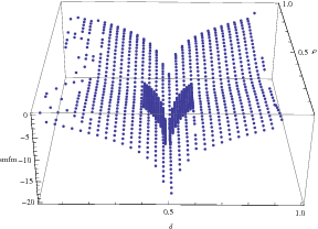
   Figure 1: $\Sigma_{T}=\Sigma_{F}=\frac{k}{2}$: $-\infty$ is obtained only when $\delta=\frac{1}{2}$.

2. setting $\Sigma_{T}=k\eta_{T}$ and $\Sigma_{F}=k\eta_{F}$: once more, only $\delta=\frac{1}{2}$ seems to make $\frac{F_{2}}{F_{1}^{2}}=1$, cf. figure 2.

   

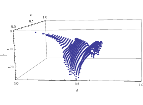
   Figure 2: $\Sigma_{T}=k\eta_{T}$ and $\Sigma_{F}=k\eta_{F}$: $-\infty$ is obtained only when $\delta=\frac{1}{2}$.

2.6.2 Implicants

An implicant is a partial assignment such that every assignment of the non-assigned variables will yield a solution. We represent the non-assigned value of variables by a $*$. We performed the calculations on implicants with the hope that their variance might be lower than the solutions’.

Preliminaries.

1. the domain of values is $D=\left\{0,1,*\right\}$; given a solution, we call $\delta$ the fraction of variables assigned $1$ and $\alpha$ the fraction of variables assigned $*$; constraints 4 and 5 become:

   $$\delta = \mu_{1,1}+\mu_{1,0}+\mu_{1,*}$$

   $$\delta = \mu_{1,1}+\mu_{0,1}+\mu_{*,1}$$

   $$\alpha = \mu_{*,1}+\mu_{*,0}+\mu_{*,*}$$

   $$\alpha = \mu_{1,*}+\mu_{0,*}+\mu_{*,*}$$

   $$1-\delta-\alpha = \mu_{0,0}+\mu_{0,1}+\mu_{0,*}$$

   $$1-\delta-\alpha = \mu_{0,0}+\mu_{1,0}+\mu_{*,0}\enskip,$$

   so, if we define $\mu=\mu_{*,*}$, $\nu=\mu_{1,1}$, $\pi=\mu_{1,*}$ and $\pi^{{}^{\prime}}=\mu_{*,1}$, we have

   $$\mu_{1,0} = \delta-\nu-\pi$$

   $$\mu_{0,1} = \delta-\nu-\pi^{{}^{\prime}}$$

   $$\mu_{*,0} = \alpha-\mu-\pi^{{}^{\prime}}$$

   $$\mu_{0,*} = \alpha-\mu-\pi$$

   $$\mu_{0,0} = 1-2\delta-2\alpha+\mu+\nu+\pi+\pi^{{}^{\prime}}\enskip;$$

2. the set of signs is $S=\left\{+,-\right\}$; we call $\rho$ the fraction of positive occurrences;

3. the set of truth values is $\mathcal{V}=\left\{T,F,*\right\}$ and the truth table is: $+$ $-$ $0$ $F$ $T$ $1$ $T$ $F$ $*$ $*$ $*$ ; so

   $$\eta_{T} = \rho\delta+\left(1-\rho\right)\left(1-\delta-\alpha\right)$$

   $$\eta_{F} = \left(1-\rho\right)\delta+\rho\left(1-\delta-\alpha\right)$$

   $$\eta_{*} = \alpha$$

   and

   $$\varepsilon_{T,T} = \rho\nu+\left(1-\rho\right)\left(1-2\delta-2\alpha+\mu+\nu+\pi+\pi^{{}^{\prime}}\right)$$

   $$\varepsilon_{T,F} = \rho\left(\delta-\nu-\pi\right)+\left(1-\rho\right)\left(\delta-\nu-\pi^{{}^{\prime}}\right)$$

   $$\varepsilon_{F,T} = \rho\left(\delta-\nu-\pi^{{}^{\prime}}\right)+\left(1-\rho\right)\left(\delta-\nu-\pi\right)$$

   $$\varepsilon_{F,F} = \rho\left(1-2\delta-2\alpha+\mu+\nu+\pi+\pi^{{}^{\prime}}\right)+\left(1-\rho\right)\nu$$

   $$\varepsilon_{*,*} = \mu$$

   $$\varepsilon_{T,*} = \rho\pi+\left(1-\rho\right)\left(\alpha-\mu-\pi\right)$$

   $$\varepsilon_{*,T} = \rho\pi^{{}^{\prime}}+\left(1-\rho\right)\left(\alpha-\mu-\pi^{{}^{\prime}}\right)$$

   $$\varepsilon_{F,*} = \rho\left(\alpha-\mu-\pi\right)+\left(1-\rho\right)\pi$$

   $$\varepsilon_{*,F} = \rho\left(\alpha-\mu-\pi^{{}^{\prime}}\right)+\left(1-\rho\right)\pi^{{}^{\prime}}\enskip;$$

4. a clause type is allowed iff it contains at least one $T$.

Condition for $\varepsilon_{v,w}=\eta_{v}\eta_{w}$ at the Independence Point.

The independence point is defined by $\mu=\alpha^{2}$, $\nu=\delta^{2}$ and $\pi=\pi^{{}^{\prime}}=\alpha\delta$. So at this point we have:

$$\varepsilon_{T,T} = \rho\delta^{2}+\left(1-\rho\right)\left(1-\delta-\alpha\right)^{2}$$

$$\varepsilon_{T,F}=\varepsilon_{F,T} = \delta\left(1-\delta-\alpha\right)$$

$$\varepsilon_{F,F} = \rho\left(1-\delta-\alpha\right)^{2}+\left(1-\rho\right)\delta^{2}$$

$$\varepsilon_{*,*} = \alpha^{2}=\eta_{*}^{2}$$

$$\varepsilon_{T,*}=\varepsilon_{*,T} = \alpha\left(\rho\delta+\left(1-\rho\right)\left(1-\delta-\alpha\right)\right)=\eta_{T}\eta_{*}$$

$$\varepsilon_{F,*}=\varepsilon_{*,F} = \alpha\left(\rho\left(1-\delta-\alpha\right)+\left(1-\rho\right)\delta\right)=\eta_{F}\eta_{*}\enskip.$$

The first thing to notice is that all identities involving $*$ satisfy $\varepsilon_{v,w}=\eta_{v}\eta_{w}$. The second thing to notice is that if $\varepsilon_{T,F}=\eta_{T}\eta_{F}$, then the three remaining identities follow, because $\varepsilon_{T,F}+\varepsilon_{T,T}+\varepsilon_{T,*}=\eta_{T}$ etc.

$$\varepsilon_{T,F}-\eta_{T}\eta_{F} = \delta\left(1-\delta-\alpha\right)-\left(\rho\delta+\left(1-\rho\right)\left(1-\delta-\alpha\right)\right)\left(\left(1-\rho\right)\delta+\rho\left(1-\delta-\alpha\right)\right)$$

$$= \delta\left(1-\delta-\alpha\right)-\rho\left(1-\rho\right)\left(\delta^{2}+\left(1-\delta-\alpha\right)^{2}\right)-\left(\rho^{2}+\left(1-\rho\right)^{2}\right)\delta\left(1-\delta-\alpha\right)$$

$$= 2\rho\left(1-\rho\right)\delta\left(1-\delta-\alpha\right)-\rho\left(1-\rho\right)\left(\delta^{2}+\left(1-\delta-\alpha\right)^{2}\right)$$

$$= -\rho\left(1-\rho\right)\left(2\delta+\alpha-1\right)^{2}\enskip.$$

Consequently, $\varepsilon_{T,F}\leq\eta_{T}\eta_{F}$, with equality iff $\rho\in\left\{0,1\right\}$ or $\delta=\frac{1-\alpha}{2}$.

We discard the particular case of $\rho\in\left\{0,1\right\}$ (which corresponds to monotone k-SAT, always trivially satisfiable). It turns out that as soon as $\delta\neq\frac{1-\alpha}{2}$, we could not make the Second Moment Method work.

On the other hand, when $\delta=\frac{1-\alpha}{2}$ we could make the Second Moment Method work.

Remark 8.

Setting $\alpha=0$ corresponds in fact to solutions (which are some trivial implicants), thus to some extent we get back to the $\delta=\frac{1}{2}$ condition. But is there a positive $\alpha$ yielding a better lower bound than $\alpha=0$?

Condition for the Second Moment Method to Work at $\delta=\frac{1-\alpha}{2}$.

As mentioned in section 2.5, stationarity of the independence point implies that $\frac{\partial\Lambda}{\partial\mu}=\frac{\partial\Lambda}{\partial\nu}=\frac{\partial\Lambda}{\partial\pi}=\frac{\partial\Lambda}{\partial\pi^{{}^{\prime}}}=0$.

Using equation 11, i.e.

$$\frac{\partial\Lambda}{\partial\mu} = -\sum_{\left(a,b\right)\in D^{2}}\frac{\partial\mu_{a,b}}{\partial\mu}\ln\mu_{a,b}+c\sum_{\left(a,b\right)\in D^{2}}\frac{\partial\mu_{a,b}}{\partial\mu}\sum_{s\in S}\rho_{s}\frac{\Xi_{a\otimes s,b\otimes s}}{\varepsilon_{a\otimes s,b\otimes s}}\enskip,$$

we get:

$$\frac{\partial\Lambda}{\partial\mu} = \ln\frac{\mu_{*,0}\mu_{0,*}}{\mu_{*,*}\mu_{0,0}}$$

$$+c\left(\left(1-\rho\right)\left(\frac{\Xi_{T,T}}{\varepsilon_{T,T}}+\frac{\Xi_{*,*}}{\eta_{*,*}}-\frac{\Xi_{T,*}}{\varepsilon_{T,*}}-\frac{\Xi_{*,T}}{\varepsilon_{*,T}}\right)+\rho\left(\frac{\Xi_{F,F}}{\varepsilon_{F,F}}+\frac{\Xi_{*,*}}{\eta_{*,*}}-\frac{\Xi_{F,*}}{\varepsilon_{F,*}}-\frac{\Xi_{*,F}}{\varepsilon_{*,F}}\right)\right)\enskip;$$

$$\frac{\partial\Lambda}{\partial\nu} = \ln\frac{\mu_{1,0}\mu_{0,1}}{\mu_{1,1}\mu_{0,0}}+c\left(\frac{\Xi_{T,T}}{\varepsilon_{T,T}}+\frac{\Xi_{F,F}}{\varepsilon_{F,F}}-\frac{\Xi_{T,F}}{\varepsilon_{T,F}}-\frac{\Xi_{F,T}}{\varepsilon_{F,T}}\right)\enskip;$$

$$\frac{\partial\Lambda}{\partial\pi} = \ln\frac{\mu_{1,0}\mu_{0,*}}{\mu_{1,*}\mu_{0,0}}$$

$$+c\left(\left(1-\rho\right)\left(\frac{\Xi_{T,T}}{\varepsilon_{T,T}}+\frac{\Xi_{F,*}}{\varepsilon_{F,*}}-\frac{\Xi_{F,T}}{\varepsilon_{F,T}}-\frac{\Xi_{T,*}}{\varepsilon_{T,*}}\right)+\rho\left(\frac{\Xi_{F,F}}{\varepsilon_{F,F}}+\frac{\Xi_{T,*}}{\varepsilon_{T,*}}-\frac{\Xi_{T,F}}{\varepsilon_{T,F}}-\frac{\Xi_{F,*}}{\varepsilon_{F,*}}\right)\right)\enskip;$$

$$\frac{\partial\Lambda}{\partial\pi^{{}^{\prime}}} = \ln\frac{\mu_{0,1}\mu_{*,0}}{\mu_{*,1}\mu_{0,0}}$$

$$+c\left(\left(1-\rho\right)\left(\frac{\Xi_{T,T}}{\varepsilon_{T,T}}+\frac{\Xi_{*,F}}{\varepsilon_{*,F}}-\frac{\Xi_{T,F}}{\varepsilon_{T,F}}-\frac{\Xi_{*,T}}{\varepsilon_{*,T}}\right)+\rho\left(\frac{\Xi_{F,F}}{\varepsilon_{F,F}}+\frac{\Xi_{*,T}}{\varepsilon_{*,T}}-\frac{\Xi_{F,T}}{\varepsilon_{F,T}}-\frac{\Xi_{*,F}}{\varepsilon_{*,F}}\right)\right)\enskip.$$

We consider the independence point, thus $\mu_{a,b}=\delta_{a}\delta_{b}$. Assuming symmetry of occurrences, we may use independence of surfaces (cf. fact 3); moreover, using condition $\varepsilon_{v,w}=\eta_{v}\eta_{w}$, we get that:

$$\frac{\partial\Lambda}{\partial\mu} = c\left(\left(1-\rho\right)\left(\frac{\Sigma_{T}}{\eta_{T}}-\frac{\Sigma_{*}}{\eta_{*}}\right)^{2}+\rho\left(\frac{\Sigma_{F}}{\eta_{F}}-\frac{\Sigma_{*}}{\eta_{*}}\right)^{2}\right)\enskip;$$

$$\frac{\partial\Lambda}{\partial\nu} = c\left(\frac{\Sigma_{T}}{\eta_{T}}-\frac{\Sigma_{F}}{\eta_{F}}\right)^{2}\enskip;$$

$$\frac{\partial\Lambda}{\partial\pi}=\frac{\partial\Lambda}{\partial\pi^{{}^{\prime}}} = c\left(\left(1-\rho\right)\left(\frac{\Sigma_{T}}{\eta_{T}}-\frac{\Sigma_{F}}{\eta_{F}}\right)\left(\frac{\Sigma_{T}}{\eta_{T}}-\frac{\Sigma_{*}}{\eta_{*}}\right)+\rho\left(\frac{\Sigma_{F}}{\eta_{F}}-\frac{\Sigma_{T}}{\eta_{T}}\right)\left(\frac{\Sigma_{F}}{\eta_{F}}-\frac{\Sigma_{*}}{\eta_{*}}\right)\right)\enskip.$$

Canceling out these derivatives yields:

$$\frac{\Sigma_{*}}{\eta_{*}} = \frac{\Sigma_{T}}{\eta_{T}}=\frac{\Sigma_{F}}{\eta_{F}}\enskip.$$

Since we assume $\delta=\frac{1-\alpha}{2}$, we have $\eta_{T}=\eta_{F}=\frac{1-\alpha}{2}$; moreover $\eta_{*}=\alpha$. Thus $\Sigma_{T}=\Sigma_{F}=k\frac{1-\alpha}{2}$ and $\Sigma_{*}=k\alpha$.

It turns out that this condition is sufficient to make the Second Moment Method work, and numerically we found the critical ratios laid in table 1 for standard 3-SAT with symmetry of occurrences at $\rho=\frac{1}{2}$.

Table 1: Critical ratios $c$ of implicants obtained for a given $\alpha$ (and the corresponding choice of the free $\beta$ parameters).

$\alpha$	$c$	$\beta_{TFF}$	$\beta_{TTF}$	$\beta_{T**}$	ratio $c$ of [3]
$0.001$	$2.81$	$0.195$	$0.10867$	$3.33\times 10^{-5}$	$4.5$
$0.01$	$2.77$	$0.1942$	$0.098833$	$3.33\times 10^{-5}$	$4.5$
$0.05$	$2.52$	$0.17767$	$0.08167$	$0.001633$	$2$
$0.08$	$2.32$	$0.1633$	$0.07$	$0.00233$	$1.5$
$0.11$	$2.13$	$0.1533$	$0.05467$	$0.0033$	$1$
$0.15$	$1.88$	$0.13833$	$0.041$	$0.012$	-
$0.2$	$1.59$	$0.1233$	$0.02567$	$0.02833$	-
$0.25$	$1.31$	$0.10833$	$0.0133$	$0.04767$	-
$0.333$	$0.89$	$0.094433$	$3.33\times 10^{-5}$	$0.094167$	-

These values are to be compared with those of Boufkhad & Dubois - 1999 [3], who proved for example that at the ratio $c=4.5$, any satisfiable instance will have prime implicants with $\alpha=0.01$. Combined with the lower bound of $3.52$ of [8] and [6], this proves that such implicants exist almost surely when $c\leq 3.52$.

Thus in the range $c\in\left(2.81,3.52\right)$ Boufkhad & Dubois prove that implicants with $\alpha=0.01$ exist. However, in the range $c\leq 2.81$ the Second Moment Method enable us to establish the existence of implicants with a $\alpha$ significantly greater than Boufkhad & Dubois’s.

How can we interpret the fact that the critical $c$ obtained decreases with $\alpha$? Looking at the set of allowed types of clauses:

$$\mathcal{T} = \left\{TTT,TTF,TFT,FTT,TFF,FTF,FFT,TT*,T*T,*TT,T**,*T*,**T\right\}$$

$$\cup\left\{TF*,T*F,FT*,F*T,*TF,*FT\right\}\enskip,$$

we can see that there are $27$ $T$’s, $15$ $F$’s and $15$ $*$’s. Thus when $*$’s are present, the ratio $T/F$ is $\frac{27}{15}=1.8$. Without $*$’s, $T/F$ would be $\frac{12}{9}\simeq 1.33$ (see section 2.7.2). Now, since the Second Moment Method requires $\Sigma_{T}=\Sigma_{F}$, we can see that it is all the more artificial as $T/F$ is large. Thus adding $*$’s should cut down the Second Moment Method’s performance.

2.7 Confrontation of the Second Moment Method with Reality

Using SATLab, we investigate the behavior of real solutions and we emphasize how it differs from the conditions required by the Second Moment Method that we laid down just above.

Based on numerical calculations of figures 1 and 2, we conjectured in section 2.5 that the Second Moment Method might work only if $\varepsilon_{v,w}=\eta_{v}\eta_{w}$. In this setting we showed that the independence point defined by $\mu_{a,b}=\delta_{a}\delta_{b}$ and $\gamma_{t,u}=\beta_{t}\beta_{u}$ must be a maximum of $T_{2}$, the second moment. This led us in section 2.6.1 to the following necessary condition for the Second Moment Method to work on boolean solutions: $\delta=\frac{1}{2}$.

Now using SATLab, we are going to give experimental evidence that:

• real solutions of standard 3-SAT violate all of these conditions: they are not independent at all!

• real solutions of standard 3-NAE-SAT seem to be rather independent.

These observations may explain why the Second Moment Method performs so poorly on standard 3-SAT (cf. section 2.6.1) whereas it works pretty well on 3-NAE-SAT (cf. Achlioptas & Moore - 2002 [1]).

2.7.1 Distances between Solutions

It turns out that in random 3-SAT, solutions are correlated with respect to their Hamming distances. Namely their Hamming distances are not centered around $50\%$ contrary to solutions of random 3-NAE-SAT, but narrower to each other (cf. figure 3).

What we mean by Hamming similarity between two assignments is just the proportion of variables assigned the same value in both assignments. We took all couples of different solutions in a sample of random solutions output by a solver, and we plotted the frequency of the Hamming similarity.

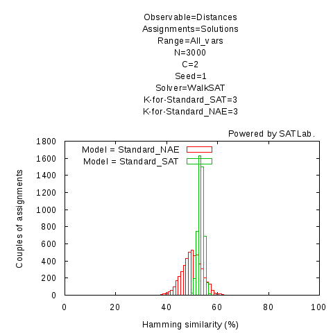
Figure 3: Hamming similarity among solutions in NAE-SAT and in SAT.

To have a more precise insight into Hamming similarity, we separated fixed and free variables. Let us recall that a variable is free iff flipping it yields another solution. We can notice that Hamming similarity is significantly greater among fixed variables than among free variables (see figure 4), and that it increases with $c$ for both types of variables (see figures 5 and 6).

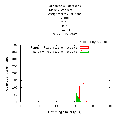
Figure 4: Hamming similarity is greater among fixed variables.

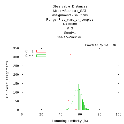
Figure 5: Hamming similarity among free variables increases with $c$.

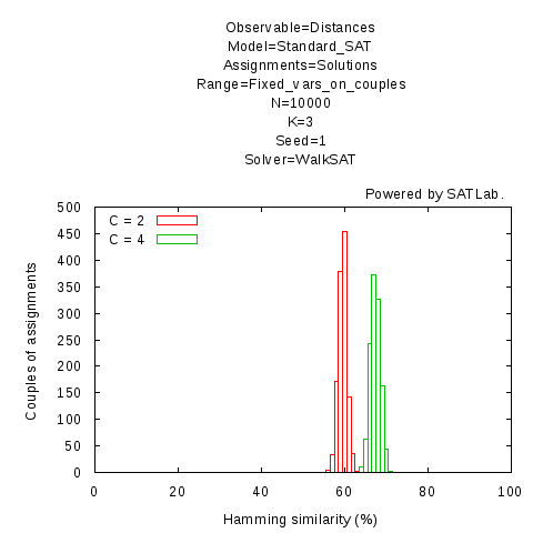
Figure 6: Hamming similarity among fixed variables increases with $c$.

2.7.2 Surface of True Literals

What we call true surface is the scaled number of true occurrences of literals. We can see a fundamental difference between the true surface of fixed variables and the true surface of free variables. Namely the true surface of fixed variables decreases with $c$ (figure 7) whereas the true surface of free variables increases with $c$ (figure 8). Note that both quantities converge to roughly $0.56$ (i.e. roughly $\frac{4}{7}$) when $c$ approaches the threshold ratio, whereas in section 2.6.1 we got the following condition: $\Sigma_{T}=\Sigma_{F}=\frac{k}{2}$ to make the Second Moment Method work.

We interpret the ratio $\frac{4}{7}$ as follows: the allowed types of clauses are

$$\left\{TTT,TTF,TFT,FTT,TFF,FTF,FFT\right\}\enskip,$$

which amounts to $12$ $T$’s and $9$ $F$’s. Now $\frac{12}{12+9}=\frac{12}{21}=\frac{4}{7}$.

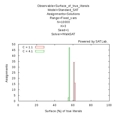
Figure 7: The true surface of fixed variables decreases with $c$.

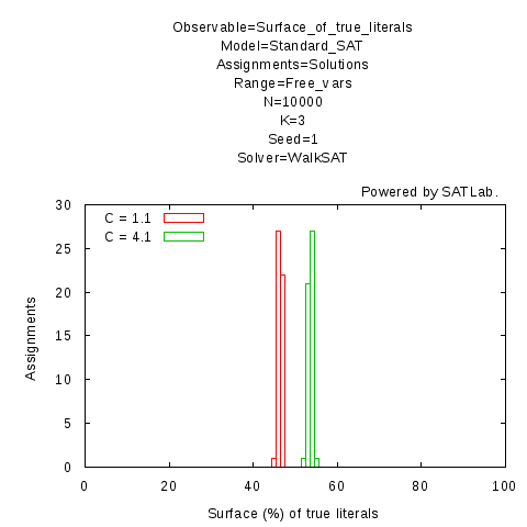
Figure 8: The true surface of free variables increases with $c$.

2.7.3 Non-Independence of True / False Surfaces

Let us consider two solutions $S_{1}$ and $S_{2}$. We denote by $\Sigma_{F}$ the false surface under solution $S_{1}$, $\Sigma_{T}$ the true surface under solution $S_{2}$, and $\Xi_{FT}$ the surface which is false under $S_{1}$ and true under $S_{2}$. In a given sample of random solutions, we took all couples of different solutions $\left(S_{1},S_{2}\right)$ and computed the ratio $\frac{\Sigma_{F}\Sigma_{T}}{k\Xi_{FT}}$; the histogram in figure 9 plots the frequency of this ratio for the solutions of two different models of formulas: random 3-NAE-SAT and random 3-SAT. Although some independence seems to exist in 3-NAE-SAT (i.e. the ratio is centered around $1$), it can be seen that there is no independence of these surfaces for random 3-SAT.

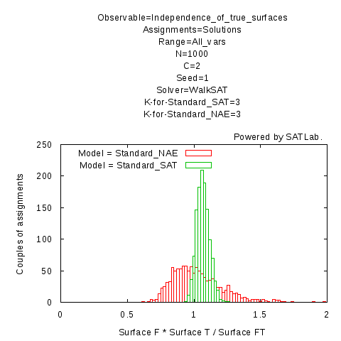
Figure 9: (Non-)independence of surfaces in NAE-SAT and in SAT.

To have a more precise insight into the non-independence, we separated fixed and free variables. Let us recall that a variable is free iff flipping it yields another solution. We can notice that non-independence comes from both free and fixed variables, but rather from fixed variables than from free variables, cf. figure 10.

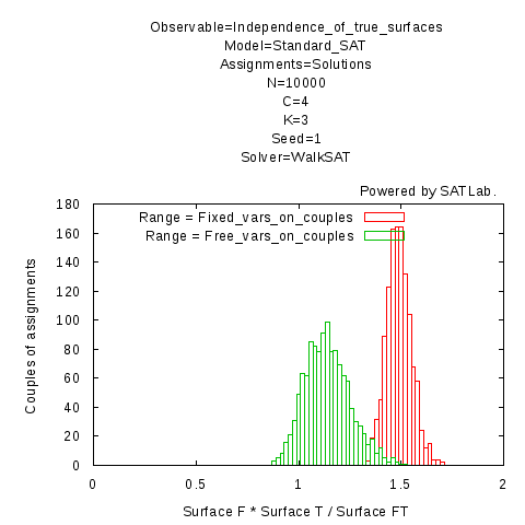
Figure 10: The non-independence of surfaces comes rather from fixed variables.

2.7.4 Non-Independence of Clauses Types

Here what we call clause type is the number of true occurrences of variables in the clause. Let us consider two solutions $S_{1}$ and $S_{2}$. We denote by $\beta_{1}$ the proportion of uniquely satisfied clauses under solution $S_{1}$, $b_{1}$ the proportion of uniquely satisfied clauses under solution $S_{2}$, and $\gamma_{1,1}$ the proportion of clauses which are uniquely satisfied under $S_{1}$ and under $S_{2}$. In a given sample of random solutions, we took all couples of different solutions $\left(S_{1},S_{2}\right)$ and computed the ratio $\frac{\beta_{1}b_{1}}{\gamma_{1,1}}$; the histogram in figure 11 plots the frequency of this ratio for the solutions of two different kinds of assignments: solutions of a random 3-NAE-SAT formula and solutions of a random 3-SAT formula. Although independence seems to happen among solutions of random 3-NAE-SAT (i.e. the ratio is centered around $1$), it can be seen that there is no independence in random 3-SAT.

In real instances we can assume symmetry of occurrences, in the sense of section 2.1.6; so in the light of fact 3, we could conclude from the non-independence of surfaces observed in section 2.7.3 that in the real solutions of 3-SAT independence of clauses types would not hold.

Figure 11: (Non-)independence of uniquely satisfied clauses in NAE-SAT and in SAT.

3 Second Moment Method on Distributional Random k-SAT

Using the standard distributional model instead of the standard drawing model yields better upper bounds on the satisfiability threshold. Moreover, we would like to gain some more control over the proportion of variables assigned $1$ according to the imbalance between their positive and negative occurrences. Namely, a variable is all the more expected to be assigned $1$ in a solution as it has more positive occurrences, and vice-versa. At least this seems to happen on real solutions, see figure 13 in section 3.6.1.

That is the reasons why we are going to implement the Second Moment Method in the distributional model.

In this section we follow roughly the same outline than in section 2, but we focus on solutions only; we only emphasize the major differences with respect to the general framework of section 2.

3.1 Preliminaries

3.1.1 Occurrences and Signs

We still have $n$ variables. We denote by $d_{p,q}$ the fraction of variables having $p$ positive and $q$ negative occurrences.

$$\sum_{\left(p,q\right)\in\boldsymbol{N}^{2}}d_{p,q} = 1\enskip;$$

$$\sum_{\left(p,q\right)\in\boldsymbol{N}^{2}}\left(p+q\right)d_{p,q} = kc\enskip.$$

Occurrences and signs of variables are determined a priori.

We ought to consider light and heavy variables $\mathcal{L}$ and $\mathcal{H}$ (cf. [4]). In fact we are going not to worry about that, because they make the calculation heavier, and in the end we shall see that there is no need to be rigorous since we only have negative results.

3.1.2 Values

Given a boolean assignment, we denote by $\delta_{p,q}$ the proportion of variables with $p$ positive and $q$ negative occurrences which are assigned $1$. Thus the proportion of variables with $p$ positive and $q$ negative occurrences which are assigned $0$ is $1-\delta_{p,q}$.

Given two assignments $S_{1}$ and $S_{2}$, for all $\left(a,b\right)\in D^{2}$, considering variables with $p$ positive and $q$ negative occurrences, we denote by:

• $\lambda_{p,q}$ the proportion of variables which are assigned $1$ in $S_{1}$ and $S_{2}$;

• $\mu_{p,q}$ the proportion of variables which are assigned $1$ in $S_{1}$ and $0$ in $S_{2}$;

• $\mu_{p,q}^{{}^{\prime}}$ the proportion of variables which are assigned $0$ in $S_{1}$ and $1$ in $S_{2}$;

• $\nu_{p,q}$ the proportion of variables which are assigned $0$ in $S_{1}$ and $S_{2}$.

We have the following constraints:

$$\delta_{p,q} = \lambda_{p,q}+\mu_{p,q}$$

$$\delta_{p,q} = \lambda_{p,q}+\mu_{p,q}^{{}^{\prime}}$$

$$1-\delta_{p,q} = \mu_{p,q}+\nu_{p,q}$$

$$1-\delta_{p,q} = \mu_{p,q}^{{}^{\prime}}+\nu_{p,q}$$

thus

$$\lambda_{p,q} = \delta_{p,q}-\mu_{p,q}$$

$$\mu_{p,q}^{{}^{\prime}} = \mu_{p,q}$$

$$\nu_{p,q} = 1-\delta_{p,q}-\mu_{p,q}$$

which enables us to work only with $\mu_{p,q}$.

3.1.3 Truth Values

$$\eta_{T} = \frac{1}{kc}\sum_{\left(p,q\right)\in\boldsymbol{N}^{2}}\left(p\delta_{p,q}+q\left(1-\delta_{p,q}\right)\right)d_{p,q}$$

$$\eta_{F} = \frac{1}{kc}\sum_{\left(p,q\right)\in\boldsymbol{N}^{2}}\left(q\delta_{p,q}+p\left(1-\delta_{p,q}\right)\right)d_{p,q}$$

$$\varepsilon_{T,T} = \frac{1}{kc}\sum_{\left(p,q\right)\in\boldsymbol{N}^{2}}\left(p\left(\delta_{p,q}-\mu_{p,q}\right)+q\left(1-\delta_{p,q}-\mu_{p,q}\right)\right)d_{p,q}$$

$$\varepsilon_{F,F} = \frac{1}{kc}\sum_{\left(p,q\right)\in\boldsymbol{N}^{2}}\left(q\left(\delta_{p,q}-\mu_{p,q}\right)+p\left(1-\delta_{p,q}-\mu_{p,q}\right)\right)d_{p,q}$$

$$\varepsilon_{T,F}=\varepsilon_{F,T} = \frac{1}{kc}\sum_{\left(p,q\right)\in\boldsymbol{N}^{2}}\left(p+q\right)\mu_{p,q}d_{p,q}$$

3.1.4 Types of Clauses and Surfaces

We keep the same definitions as in section 2.1.

However, some extra constraints on surfaces occur in the distributional model, because here all occurrences and signs of variables are determined a priori:

$$\Sigma_{v} = k\eta_{v}\enskip;$$ (16)

$$\Xi_{v,w} = k\varepsilon_{v,w}\enskip.$$ (17)

3.2 Expression of the First Moment

The first moment of the number $X$ of solutions can be split up into the following factors: total number of assignments and probability for an assignment to be a solution.

1. total number of assignments: choose subsets of variables assigned $0$ or $1$:
   $\prod_{\left(p,q\right)\in\mathcal{L}}{d_{p,q}n\choose\delta_{p,q}d_{p,q}n}$;

2. probability for an assignment to be a solution:

   1. number of satisfied formulas:

      1. we give each clause an allowed type $t\in\mathcal{T}$: ${cn\choose\dots\left(\beta_{t}cn\right)_{t\in\mathcal{T}}\dots}$

      2. we find a permutation of the true literals into the true boxes and a permutation of the false literals into the false boxes: $\left(\eta_{T}kcn\right)!\left(\eta_{F}kcn\right)!$

   2. total number of formulas, i.e. number of permutations of the occurrences of literals into the boxes: $\left(kcn\right)!$

We denote by $\mathcal{P}$ the set of all families of non-negative numbers $\left(\left(\delta_{p,q}\right)_{\left(p,q\right)\in\mathcal{L}},\left(\beta_{t}\right)_{t\in\mathcal{T}}\right)$ satisfying constraint 7. We denote by $\mathcal{I}\left(n\right)$ the intersection of $\mathcal{P}$ with the multiples of $\frac{1}{n}$; we get the following expression of the first moment:

$$\mathrm{E}X = \sum_{\left(\left(\delta_{p,q}\right)_{\left(p,q\right)\in\mathcal{L}},\left(\beta_{t}\right)_{t\in\mathcal{T}}\right)\in\mathcal{I}\left(n\right)}T_{1}\left(n\right)$$

where

$$T_{1}\left(n\right) = \frac{\prod_{\left(p,q\right)\in\mathcal{L}}{d_{p,q}n\choose\delta_{p,q}d_{p,q}n}{cn\choose\dots\left(\beta_{t}cn\right)_{t\in\mathcal{T}}\dots}}{{kcn\choose\eta_{T}kcn}}\enskip.$$

The exponential equivalent of $T_{1}\left(n\right)$ is $T_{1}^{n}$, where

$$T_{1} = \frac{1}{\prod_{\left(p,q\right)\in\mathcal{L}^{2}}\delta_{p,q}^{\delta_{p,q}d_{p,q}}}\left(\frac{\left(\eta_{T}^{\eta_{T}}\eta_{F}^{\eta_{F}}\right)^{k}}{\prod_{t\in\mathcal{T}}\beta_{t}^{\beta_{t}}}\right)^{c}\enskip.$$

3.3 Expression of the Second Moment

The second moment of $X$ can be split up into the following factors: total number of assignments and probability for an assignment to be a solution.

1. total number of assignments: choose subsets of variables assigned $0$ or $1$:
   $\prod_{\left(p,q\right)\in\mathcal{L}}{d_{p,q}n\choose\lambda_{p,q}d_{p,q}n,\mu_{p,q}d_{p,q}n,\mu_{p,q}d_{p,q}n,\nu_{p,q}d_{p,q}n}$;

2. probability for an assignment to be a solution:

   1. number of satisfied formulas:

      1. we give each clause two allowed types: ${cn\choose\dots\left(\gamma_{t,u}cn\right)_{\left(t,u\right)\in\mathcal{T}^{2}}\dots}$

      2. we find a permutation of the literals into the corresponding boxes:
         $\left(\varepsilon_{T,T}kcn\right)!\left(\varepsilon_{T,F}kcn\right)!\left(\varepsilon_{F,T}kcn\right)!\left(\varepsilon_{F,F}kcn\right)!$

   2. total number of formulas, i.e. number of permutations of the occurrences of literals into the boxes: $\left(kcn\right)!$

We denote by $\mathcal{P}_{2}$ the set of all families of non-negative numbers $\left(\left(\mu_{p,q}\right)_{\left(p,q\right)\in\mathcal{L}},\left(\gamma_{t,u}\right)_{\left(t,u\right)\in\mathcal{T}^{2}}\right)$ satisfying constraints 8 and 9. We denote by $\mathcal{I}_{2}\left(n\right)$ the intersection of $\mathcal{P}_{2}$ with the multiples of $\frac{1}{n}$; we get the following expression of the second moment:

$$\mathrm{E}X^{2} = \sum_{\left(\left(\mu_{p,q}\right)_{\left(p,q\right)\in\mathcal{L}},\left(\gamma_{t,u}\right)_{\left(t,u\right)\in\mathcal{T}^{2}}\right)\in\mathcal{I}_{2}\left(n\right)}T_{2}\left(n\right)$$

where

$$T_{2}\left(n\right) = \frac{\prod_{\left(p,q\right)\in\mathcal{L}}{d_{p,q}n\choose\lambda_{p,q}d_{p,q}n,\mu_{p,q}d_{p,q}n,\mu_{p,q}d_{p,q}n,\nu_{p,q}d_{p,q}n}{cn\choose\dots\left(\gamma_{t,u}cn\right)_{\left(t,u\right)\in\mathcal{T}^{2}}\dots}}{{kcn\choose\varepsilon_{T,T}kcn,\varepsilon_{T,F}kcn,\varepsilon_{F,T}kcn,\varepsilon_{F,F}kcn}}\enskip.$$

The exponential equivalent of $T_{2}\left(n\right)$ is $T_{2}^{n}$, where

$$T_{2} = \frac{1}{\prod_{\left(p,q\right)\in\mathcal{L}}\left(\left(\delta_{p,q}-\mu_{p,q}\right)^{\delta_{p,q}-\mu_{p,q}}\mu_{p,q}^{2\mu_{p,q}}\left(1-\delta_{p,q}-\mu_{p,q}\right)^{1-\delta_{p,q}-\mu_{p,q}}\right)^{d_{p,q}}}$$

$$\cdot\left(\frac{\left(\varepsilon_{T,T}^{\varepsilon_{T,T}}\varepsilon_{T,F}^{\varepsilon_{T,F}}\varepsilon_{F,T}^{\varepsilon_{F,T}}\varepsilon_{F,F}^{\varepsilon_{F,F}}\right)^{k}}{\prod_{\left(t,u\right)\in\mathcal{T}^{2}}\gamma_{t,u}^{\gamma_{t,u}}}\right)^{c}\enskip.$$

3.4 Expression of the Lagrangian

When the parameters of the first moment (i.e. $\left(\delta_{p,q}\right)_{\left(p,q\right)\in\mathcal{L}},\left(\beta_{t}\right)_{t\in\mathcal{T}}$) are chosen, $T_{2}$ must be maximized under constraints 8 and 9. That leads us to use the Lagrange multipliers method. In order to make the forthcoming maximization easier, we introduce some extra variables $\psi_{v,w}$ which are going to simulate $\varepsilon_{v,w}$. The reason for this is that $\varepsilon_{v,w}$ contains $\mu_{p,q}$, but we need the expression of $\mu_{p,q}$ for our numerical calculations. So, because of equation 17, we have the following constraints:

$$k\varepsilon_{T,T}=k\psi_{T,T} = \Xi_{T,T}$$

$$k\varepsilon_{T,F}=k\psi_{T,F} = \Xi_{T,F}$$

$$k\varepsilon_{F,T}=k\psi_{F,T} = \Xi_{F,T}$$

$$k\varepsilon_{F,F}=k\psi_{F,F} = \Xi_{F,F}$$

Using the facts that $\varepsilon_{T,T}+\varepsilon_{T,F}=\eta_{T}$, $\Xi_{T,T}+\Xi_{T,F}=\Sigma_{T}$ and $\Sigma_{T}=k\eta_{T}$, we see that constraint $\varepsilon_{T,T}=\psi_{T,T}$ is redundant. Eliminating $\varepsilon_{F,T}$ and $\varepsilon_{F,F}$ as well, there remain the following 5 constraints:

$$\varepsilon_{T,F} = \psi_{T,F}$$ (18)

$$\psi_{T,T} = \eta_{T}-\psi_{T,F}$$ (19)

$$\psi_{T,F} = \frac{\Xi_{T,F}}{k}$$ (20)

$$\psi_{F,T} = \psi_{T,F}$$ (21)

$$\psi_{F,F} = \eta_{F}-\psi_{T,F}$$ (22)

So we define the following Lagrangian:

$$\Lambda = -\sum_{\left(p,q\right)\in\mathcal{L}}d_{p,q}\left(\left(\delta_{p,q}-\mu_{p,q}\right)\ln\frac{\delta_{p,q}-\mu_{p,q}}{e}+\left(1-\delta_{p,q}-\mu_{p,q}\right)\ln\frac{1-\delta_{p,q}-\mu_{p,q}}{e}\right)$$

$$-2\sum_{\left(p,q\right)\in\mathcal{L}}d_{p,q}\mu_{p,q}\ln\frac{\mu_{p,q}}{e}-c\sum_{\left(t,u\right)\in\mathcal{T}^{2}}\gamma_{t,u}\ln\frac{\gamma_{t,u}}{e}+kc\sum_{\left(v,w\right)\in\left\{T,F\right\}^{2}}\psi_{v,w}\ln\frac{\psi_{v,w}}{e}$$

$$+c\sum_{\left(v,w\right)\in\left\{T,F\right\}^{2}}\left(\ln h_{v,w}\right)\left(\Xi_{v,w}-k\psi_{v,w}\right)+kc\left(\ln y\right)\left(\psi_{T,F}-\varepsilon_{T,F}\right)$$

$$+c\sum_{t\in\mathcal{T}}\left(\ln f_{t}\right)\left(\sum_{u\in\mathcal{T}}\gamma_{t,u}-\beta_{t}\right)+c\sum_{u\in\mathcal{U}}\left(\ln g_{u}\right)\left(\sum_{t\in\mathcal{T}}\gamma_{t,u}-\beta_{u}\right)\enskip.$$

3.4.1 Derivative with respect to $\gamma_{t,u}$

$$\frac{\partial\Lambda}{\partial\gamma_{t,u}} = -c\ln\gamma_{t,u}+c\sum_{i=1}^{k}\ln h_{t_{i},u_{i}}+c\ln f_{t}+c\ln g_{u}\enskip.$$

Canceling out this derivative yields:

$$\gamma_{t,u} = f_{t}g_{u}\prod_{i=1}^{k}h_{t_{i},u_{i}}\enskip.$$ (23)

3.4.2 Derivative with respect to $\psi_{v,w}$

$$\frac{\partial\Lambda}{\partial\psi_{v,w}} = kc\ln\psi_{v,w}-kc\ln h_{v,w}+kc\left(\ln y\right)\boldsymbol{1}_{v=T\land w=F}\enskip.$$

Canceling out these derivatives yields:

$$\psi_{v,w} = h_{v,w}y^{-\boldsymbol{1}_{v=T\land w=F}}\enskip.$$ (24)

Thus constraints 18, 19, 20, 21 and 22 become:

$$\varepsilon_{T,F} = \frac{h_{T,F}}{y}$$

$$h_{T,T} = \eta_{T}-\frac{h_{T,F}}{y}$$

$$\frac{h_{T,F}}{y} = \frac{\Xi_{T,F}}{k}$$

$$h_{F,T} = \frac{h_{T,F}}{y}$$

$$h_{F,F} = \eta_{F}-\frac{h_{T,F}}{y}$$

3.4.3 Derivative with respect to $\mu_{p,q}$

$$\frac{\partial\Lambda}{\partial\mu_{p,q}} = d_{p,q}\ln\frac{\left(\delta_{p,q}-\mu_{p,q}\right)\left(1-\delta_{p,q}-\mu_{p,q}\right)}{\mu_{p,q}^{2}}-\left(p+q\right)d_{p,q}\ln y\enskip.$$ (25)

Canceling out this derivative yields:

$$\left(\delta_{p,q}-\mu_{p,q}\right)\left(1-\delta_{p,q}-\mu_{p,q}\right) = \mu_{p,q}^{2}y^{p+q}\enskip,$$

i.e.

$$\mu_{p,q}^{2}\left(1-y^{p+q}\right)-\mu_{p,q}+\delta_{p,q}\left(1-\delta_{p,q}\right) = 0\enskip.$$

Thus there are 2 cases to consider:

1. case where $y=1$ or $p+q=0$: $\mu_{p,q}=\delta_{p,q}\left(1-\delta_{p,q}\right)$;

2. case where $y\neq 1$ and $p+q\neq 0$: $\mu_{p,q}=\frac{1\pm\sqrt{1-4\left(1-y^{p+q}\right)\delta_{p,q}\left(1-\delta_{p,q}\right)}}{2\left(1-y^{p+q}\right)}$; numerically we can find solutions with $\mu_{p,q}=\frac{1-\sqrt{1-4\left(1-y^{p+q}\right)\delta_{p,q}\left(1-\delta_{p,q}\right)}}{2\left(1-y{}^{p+q}\right)}$.

3.5 Independence Point

As in section 2.5, we define the independence point by $\mu_{p,q}=\delta_{p,q}\left(1-\delta_{p,q}\right)$ and $\gamma_{t,u}=\beta_{t}\beta_{u}$. Again, we were able to make the Second Moment Method work only if $\varepsilon_{v,w}=\eta_{v}\eta_{w}$.

When $\varepsilon_{v,w}=\eta_{v}\eta_{w}$, we have $\frac{T_{2}}{T_{1}^{2}}=1$ (see proof of theorem 5) and the independence point is stationary without any extra condition (plug $h_{v,w}=\eta_{v}\eta_{w}$, $y=1$, $f_{t}=\frac{\beta_{t}}{\prod_{i=1}^{k}\eta_{t_{i}}}$, $g_{u}=\frac{\beta_{u}}{\prod_{i=1}^{k}\eta_{u_{i}}}$ into the constraints and equations 23, 24 and 25), assuming symmetry of occurrences as usual (and thus fact 3). By comparison with chapter 2, we could say that the extra condition we had there on the surfaces to make the independence point stationary corresponds here to the preliminary extra constraint 17.

Moreover, it is noteworthy that, because of fact 3 and constraint 16, the independence point violates constraint 17 when $\varepsilon_{v,w}\neq\eta_{v}\eta_{w}$.

So, what is the condition for $\varepsilon_{v,w}=\eta_{v}\eta_{w}$?

3.5.1 Condition for $\varepsilon_{v,w}=\eta_{v}\eta_{w}$ at the Independence Point

As before in section 2.6.1, the first thing to notice is that if $\varepsilon_{T,F}=\eta_{T}\eta_{F}$, then the three other identities follow, because $\varepsilon_{T,F}+\varepsilon_{T,T}=\eta_{T}$ etc.

We are grateful to Emmanuel Lepage, who gave us the main idea to compare $\varepsilon_{T,F}$ and $\eta_{T}\eta_{F}$. Let us make the following change of variables: $\delta_{p,q}=\frac{1}{2}+\delta_{p,q}^{{}^{\prime}}$:

$$\eta_{T} = \frac{1}{2}+\frac{1}{kc}\sum_{\left(p,q\right)\in\boldsymbol{N}^{2}}\left(p-q\right)\delta_{p,q}^{{}^{\prime}}d_{p,q}\enskip;$$

$$\eta_{F} = \frac{1}{2}-\frac{1}{kc}\sum_{\left(p,q\right)\in\boldsymbol{N}^{2}}\left(p-q\right)\delta_{p,q}^{{}^{\prime}}d_{p,q}\enskip;$$

$$\varepsilon_{T,F} = \frac{1}{4}-\frac{1}{kc}\sum_{\left(p,q\right)\in\boldsymbol{N}^{2}}\left(p+q\right)\delta_{p,q}^{{}^{\prime}2}d_{p,q}\enskip.$$

Thus

$$\varepsilon_{T,F}-\eta_{T}\eta_{F} = \left(\frac{1}{kc}\sum_{\left(p,q\right)\in\boldsymbol{N}^{2}}\left(p-q\right)\delta_{p,q}^{{}^{\prime}}d_{p,q}\right)^{2}-\frac{1}{kc}\sum_{\left(p,q\right)\in\boldsymbol{N}^{2}}\left(p+q\right)\delta_{p,q}^{{}^{\prime}2}d_{p,q}\enskip.$$

1. $\left(\frac{1}{kc}\sum_{\left(p,q\right)\in\boldsymbol{N}^{2}}\left(p-q\right)\delta_{p,q}^{{}^{\prime}}d_{p,q}\right)^{2}\leq\left(\frac{1}{kc}\sum_{\left(p,q\right)\in\boldsymbol{N}^{2}}\left|\left(p-q\right)\delta_{p,q}^{{}^{\prime}}\right|d_{p,q}\right)^{2}$, with equality iff
   $\left(p-q\right)\delta_{p,q}^{{}^{\prime}}$ has the same sign wherever $d_{p,q}\neq 0$;

2. Since $p,q\geq 0$, $\left|p-q\right|\leq p+q$ with equality iff $p=0$ or $q=0$;
   thus $\left(\frac{1}{kc}\sum_{\left(p,q\right)\in\boldsymbol{N}^{2}}\left|\left(p-q\right)\delta_{p,q}^{{}^{\prime}}\right|d_{p,q}\right)^{2}\leq\left(\frac{1}{kc}\sum_{\left(p,q\right)\in\boldsymbol{N}^{2}}\sqrt{p+q}^{2}\left|\delta_{p,q}^{{}^{\prime}}\right|\sqrt{d_{p,q}}^{2}\right)^{2}$, with equality iff $\delta_{p,q}^{{}^{\prime}}=0$ wherever $p\neq 0$, $q\neq 0$ and $d_{p,q}\neq 0$;

3. By the Cauchy-Schwartz inequality,

   $$\left(\frac{1}{kc}\sum_{\left(p,q\right)\in\boldsymbol{N}^{2}}\sqrt{p+q}^{2}\left|\delta_{p,q}^{{}^{\prime}}\right|\sqrt{d_{p,q}}^{2}\right)^{2}$$

   $$\leq \left(\frac{1}{kc}\sum_{\left(p,q\right)\in\boldsymbol{N}^{2}}\sqrt{p+q}^{2}\sqrt{d_{p,q}}^{2}\right)\left(\frac{1}{kc}\sum_{\left(p,q\right)\in\boldsymbol{N}^{2}}\sqrt{p+q}^{2}\left|\delta_{p,q}^{{}^{\prime}}\right|^{2}\sqrt{d_{p,q}}^{2}\right)$$

   $$= \frac{1}{kc}\sum_{\left(p,q\right)\in\boldsymbol{N}^{2}}\left(p+q\right)\delta_{p,q}^{{}^{\prime}2}d_{p,q}\enskip,$$

   with equality iff $\left|\delta_{p,q}^{{}^{\prime}}\right|$ has the same value wherever $\left(p+q\right)d_{p,q}\neq 0$.

To conclude, $\varepsilon_{T,F}\leq\eta_{T}\eta_{F}$ with equality iff ($\delta_{p,q}^{{}^{\prime}}=0$ whenever $\left(p+q\right)d_{p,q}\neq 0$) or ($\delta_{p,q}^{{}^{\prime}}$ is symmetric in $p,q$ and the model has only pure literals).

This means that in all models allowing non-pure literals (in particular the standard model having a 2D-Poisson $d_{p,q}$), $\varepsilon_{T,F}=\eta_{T}\eta_{F}$ iff $\delta_{p,q}=\frac{1}{2}$ whenever $\left(p+q\right)d_{p,q}\neq 0$.

Consequently, even in the distributional model, we encounter the very restrictive condition $\delta_{p,q}=\frac{1}{2}$ to make the Second Moment Method work.

Numerically, we found a critical ratio of $2.838$, thus very slightly above the $2.833$ obtained in the drawing model (cf section 2.6.1).

3.5.2 Attempts to evade the $\delta_{p,q}=\frac{1}{2}$ condition

The shape of $\delta_{p,q}$ on figures 13 and 14 suggested us that on real solutions $\delta_{p,q}=$$\frac{1}{1+\omega^{p-q}}$. So we tried to evade the $\omega=1$ case.

We plotted $\ln\ln\frac{F_{2}}{F_{1}^{2}}$ for different values of $\omega$, at a point satisfying constraints 8, 9, 17, 18, 19, 20, 21 and 22, for the best choice of the $\beta_{t}$’s that we found complying with constraint 16. The expected value is $-\infty$ iff $\frac{F_{2}}{F_{1}^{2}}=1$. We set the ratio $c=0.1$ (to be compared with $2.838$, where $\omega=1$ works). Only $\omega=1$ seems to make $\frac{F_{2}}{F_{1}^{2}}=1$, cf. figure 12.

Figure 12: Setting $\delta_{p,q}=$$\frac{1}{1+\omega^{p-q}}$ makes the Second Moment Method work iff $\omega=1$.

3.6 Confrontation with Reality

We are going to do the same kinds of observations through SATLab as in section 2.7 in order to figure out why the Second Moment Method still fails to give high upper bounds in the distributional model.

3.6.1 Non-Independence of Values

We focus our attention on variables with $T$ occurrences among which $U$ are positive. We denote by $d$ the average proportion of those variables assigned $1$ by a solution and $u$ the average proportion of those variables assigned $0$ and $1$ by a couple of distinct solutions. In a given sample of random solutions, we took all couples of different solutions and computed the following three quantities: $d$, $d\_d=d\left(1-d\right)$ and $u$. At independence we should have $u=d\_d$, which happens for $c=2$ (cf. figure 13) but not for $c=4$ (cf. figure 14).

Moreover we can see that $d$ is almost linear in $U$ when $c=2$ but it curves when $c=4$. Note also that the range of $U$ may be strictly included in $\left[0\dots T\right]$ (cf. figure 14). Determining the shape of $d$ might help do better calculations of first and second moments, even though in section 3.5.2 we took $\delta_{p,q}=$$\frac{1}{1+\omega^{p-q}}$ but it could not make the Second Moment Method work. It is clear however that the condition $\delta_{p,q}=\frac{1}{2}$ we encountered in section 3.5.1 does not hold on real solutions.

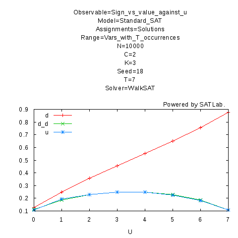
Figure 13: $\delta_{p,q}$ and $\mu_{p,q}=\delta_{p,q}\left(1-\delta_{p,q}\right)$ at $c=2$.

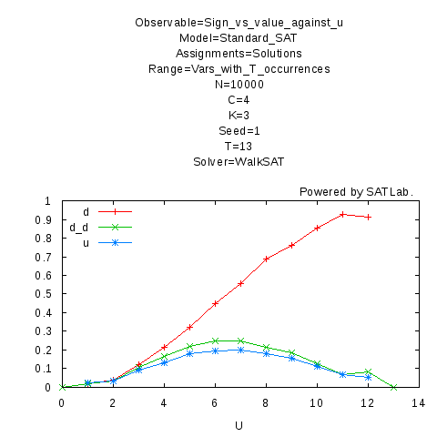
Figure 14: $\delta_{p,q}$ and $\mu_{p,q}\neq\delta_{p,q}\left(1-\delta_{p,q}\right)$ at $c=4$.

3.6.2 Non-Independence of Surfaces

We perform the same experiment as in section 2.7.3, but we restrict surfaces to variables having $T$ occurrences among which $U$ are positive. On figure 15 we can see that there is still no independence of surfaces, although the restriction of the surfaces to these variables curbs the non-independence.

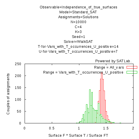
Figure 15: The distributional model slightly curbs the non-independence of surfaces.

4 Conclusion on the Second Moment Method

Contrary to the First Moment Method, which works more or less finely, the Second Moment Method will not always work. Furthermore, it is rather difficult to make it work, and we were able to make it work only under very artificial conditions with respect to reality. Moreover, even when it works, we have not been able to find strong lower bounds with it. We got stuck at $2.83$ for 3 different models (standard drawing model, implicants and standard distributional model).

However we did not prove that it is impossible to find better lower bounds with our general framework, this is just numerical experiments. Moreover our framework may not be perfect, perhaps the parameters we consider are not relevant for the Second Moment Method, so there is still hope in making the Second Moment Method work and give higher lower bounds on the threshold of 3-SAT.

References

- [1] Dimitris Achlioptas and Cristopher Moore. The asymptotic order of the random k-SAT threshold. In The 43rd Annual IEEE Symposium on Foundations of Computer Science, pages 779–788. IEEE Computer Society, 2002.
- [2] Dimitris Achlioptas and Yuval Peres. The Threshold for Random k-SAT is 2^k ln2 - O(k). JAMS: Journal of the American Mathematical Society, 17:947–973, 2004.
- [3] Yacine Boufkhad and Olivier Dubois. Length of prime implicants and number of solutions of random CNF formulae. Theoretical Computer Science, 215(1-2):1–30, 1999.
- [4] J. Díaz, Lefteris M. Kirousis, D. Mitsche, and X. Pérez-Giménez. On the satisfiability threshold of formulas with three literals per clause. Theoretical Computer Science, 410(30-32):2920–2934, 2009.
- [5] Ehud Friedgut and J. Bourgain. Sharp thresholds of graph properties, and the k-sat problem. Journal of the American Mathematical Society, 12(4):1017–1054, 1999.
- [6] M.T. Hajiaghayi and G.B. Sorkin. The satisfiability threshold of random 3-SAT is at least 3.52. IBM Research Report RC22942, 2003.
- [7] Thomas Hugel. SATLab, 2010.
- [8] A.C. Kaporis, Lefteris M. Kirousis, and E.G. Lalas. The probabilistic analysis of a greedy satisfiability algorithm. Random Structures and Algorithms, 28(4):444–480, 2006.