Trace formula for dielectric cavities II:
Regular, pseudo-integrable, and chaotic examples

Abstract

Dielectric resonators are open systems particularly interesting due to their wide range of applications in optics and photonics. In a recent paper [PRE 78, 056202 (2008)] the trace formula for both the smooth and the oscillating parts of the resonance density was proposed and checked for the circular cavity. The present paper deals with numerous shapes which would be integrable (square, rectangle, and ellipse), pseudo-integrable (pentagon) and chaotic (stadium), if the cavities were closed (billiard case). A good agreement is found between the theoretical predictions, the numerical simulations, and experiments based on organic micro-lasers.

I Introduction

Open quantum (or wave) systems are rarely integrable and therefore difficult to deal with. Over recent years, this field of research has raised many crucial questions and various systems have been investigated. Here we consider open dielectric resonators for their wide range of applications in optics and photonics vahala ; matsko . In a first paper bogomolny , the trace formula for these systems was derived in the semi-classical regime to infer their spectral features. More specifically in that paper both the expressions for the weighting coefficients of the periodic orbits and the counting function $N(k)$ (mean number of resonances with a real part of the wave number less than $k$) were obtained and demonstrated analytically for two integrable cases, the two-dimensional (2D) circular cavity and the 1D Fabry-Perot resonator. In the present paper, we consider in detail 2D dielectric cavities with different shapes where no explicit exact solution is known. We compare the predictions of formulae obtained in bogomolny with numerical simulations and experiments based on organic micro-lasers.

Resonance problems can be seen as counterparts of the scattering of an electromagnetic wave on a finite obstacle. This point of view turns out to be particularly interesting since such scattering problems have been extensively studied (see e.g. laxphillips ). Rigorous results for the scattering of a wave on convex obstacles with Dirichlet boundary conditions were proved in petkovpopov . Physical approach to these problems has been discussed in uzy . More recently some theorems were demonstrated in robert1 ; robert2 . The general structure of the resonance spectrum on a transparent smooth obstacle was studied in popovvodev .

This paper is focused on careful investigations of spectral properties for 2D convex dielectric resonators, which are the open counterparts of the so-called ’quantum billiards’. The outline of the paper is the following. The formulas obtained in bogomolny are recalled and the numerical and experimental techniques are described in Sec. II. Then different cavity shapes are explored and their properties are compared with what is known for billiards. The square, rectangle, and ellipse cases are gathered in Sec. III. We call such shapes ’regular shapes’ since the corresponding billiard problems are separable. In Sec. IV, the pentagonal dielectric cavity was chosen to illustrate a pseudo-integrable system. Eventually in Sec. V, the Bunimovich stadium is investigated as an archetype of a chaotic system. For completeness in Appendix A, the derivation of the Weyl’s law is briefly presented.

II Background: theory, numerics, and experiments

Real dielectric resonators are three-dimensional (3D) cavities requiring that the 3D vectorial Maxwell equations are used. When the cavity thickness is of the order of the wavelength, this problem can be approximated to a 2D scalar equation following the effective index model, which is widely used in photonics (see e.g. vahala and references therein). This approach has been proved to be quite efficient for our organic micro-lasers lebental ; lebental-matsko . Briefly, it assumes that the electromagnetic field can be separated in two independent polarizations, called TM (resp. TE) if the magnetic (resp. electric) field lies in the plane of the cavity ($xy$) . In this 2D approximation the Maxwell equations are reduced to the Helmholtz equation

$$(\Delta_{xy}+n^{2}k^{2})\,\psi=0$$ (1)

where $\psi$ stands for the $z$-component of the electric (resp. magnetic) field in TM (resp. TE) polarization. After resolution, all the components of the electromagnetic fields can be inferred from $\psi$. In Eq. (1) $k$ is the wave number and $n$ the effective refractive index. It is worth highlighting that the error of this approximation is not well controlled bittner_2 .

The boundary conditions in this 2D approximation are the following:

$$\psi_{1}=\psi_{2},\hskip 14.22636pt \hskip 25.6073pt\frac{\partial\psi_{1}}{\partial\nu}=\frac{\partial\psi_{2}}{\partial\nu}\hskip 28.45274pt\mbox{(TM)}$$ and

$$\psi_{1}=\psi_{2},\hskip 14.22636pt \hskip 14.22636pt\frac{1}{n^{2}}\frac{\partial\psi_{1}}{\partial\nu}=\frac{\partial\psi_{2}}{\partial\nu}\hskip 28.45274pt\mbox{(TE)}$$ and

where $\nu$ is a direction normal to the boundary and $\psi_{1}$ (resp. $\psi_{2}$) corresponds to the field inside (resp. outside) the cavity. In the case of an open system such as a dielectric cavity, the resonances are defined as the solutions of (1) with the outgoing boundary condition at infinity:

$$\psi(\vec{x})\propto e^{\mathrm{i}k|\vec{x}|}\quad|\vec{x}|\to\infty$$ (2)

Then the resonance eigenvalues, $k_{n}^{2}$, are complex with negative imaginary part

$$k_{n}^{2}=E-\frac{\mathrm{i}}{2\tau}\ .$$ (3)

$E$ is called the energy of the resonance whereas $\tau$ is its lifetime. The wave numbers of the low-loss resonances (higher quality factors) are thus located closed to the real axis.

II.1 Semiclassical trace formula

Here for simplicity, we consider only TM polarization where the functions and their normal derivative are continuous on the cavity boundary. In this case, it appears that the resonance spectrum splits into two subsets, depending on the imaginary part of the wave numbers. For one of the subsets, the wave numbers lie above a boundary

$$\gamma_{max}<\mathrm{Im}\ k_{n}<0\ ,$$ (4)

where $\gamma_{max}$ is a certain constant which depends on the cavity, and the corresponding wave functions are mainly concentrated inside the cavity. These resonances are similar to the so-called Feschbach resonances. For the second class of resonances (called shape resonances) the wave functions are mainly supported outside the cavity and the corresponding eigenvalues have large imaginary parts. For smooth convex obstacles, it was shown (see e.g. sjostrand and references therein) that they obey the inequality

$$\textrm{Im}\,k_{n}<-\,\textrm{Const}\,|\textrm{Re}\,k_{n}|^{1/3}.$$

Hereafter we will focus only on Feschbach (inner) resonances, since they are the most relevant for lasers and photonics applications. They will simply be referred to as “resonances” from now on.

The spectral density can formally be separated in two contributions

$$d(k)=\overline{d}(k)+d^{(osc)}(k)\ .$$ (5)

$\overline{d}(k)$ stands for the smooth part and is usually written through the counting function $\overline{d}(k)=\mathrm{d}\bar{N}(k)/\mathrm{d}k$ which counts how many resonances in average have a real part less than $k$ . The oscillating part, $d^{(osc)}$, can be related in the semiclassical regime $kl\gg 1$ ($l$ is any characteristic length of the cavity) to a sum over the classical periodic orbits gutzwiller .

In bogomolny , the semiclassical trace formula for open dielectric cavities was derived. It states that the counting function of dielectric resonators can be written as follows:

$$\bar{N}(k)=n^{2}\displaystyle\frac{{\cal A}k^{2}}{4\pi}+\tilde{r}(n)\displaystyle\frac{{\cal L}k}{4\pi}+{\cal O}(1)$$ (6)

where ${\cal A}$ is the area of the cavity, ${\cal L}$ its perimeter, and $\tilde{r}(n)$ a function of the refractive index involving elliptic integrals:

$$\tilde{r}(n)=1+\frac{n^{2}}{\pi}\int_{-\infty}^{\infty}\frac{\mathrm{d}t}{t^{2}+n^{2}}\,R(t)-\frac{1}{\pi}\int_{-\infty}^{\infty}\frac{\mathrm{d}t}{t^{2}+1}\,R(t)$$

with

$$R(t)=\frac{\sqrt{t^{2}+n^{2}}-\sqrt{t^{2}+1}}{\sqrt{t^{2}+n^{2}}+\sqrt{t^{2}+1}}$$

The derivation of (6) and details on $\tilde{r}(n)$ and $R(t)$ are given in Appendix A. In the following, we will compare for various shapes the prediction of (6) to the function $N(k)$ inferred from numerical simulations, and show a good agreement in all considered cases. In particular, we will stress the non trivial linear coefficient

$$\alpha^{th}=\tilde{r}(n)\displaystyle{\cal L}/4\pi$$ (7)

In this paper, in general $n=1.5$, and so $\tilde{r}(1.5)=1.025$.

The oscillating part of the trace formula is written as a sum over classical periodic orbits ($p.o.$):

$$d^{(osc)}(k)=\sum_{p.o.}\big{(}c_{p}\,e^{\mathrm{i}nkl_{p}}+c.c.\big{)}$$ (8)

where $l_{p}$ is the length of the orbit and $c_{p}$ its amplitude which depends only on classical quantities. We count a periodic orbit and the corresponding time-reversed orbit as a single orbit. The expressions for the $c_{p}$ can be derived in a standard way (see eg. gutzwiller ; bb ), using the formula of the reflected Green function given in Appendix A. As for billiard, it depends whether the orbit is isolated (i.e. unstable) or not. For an isolated periodic orbit

$$c_{p}=\frac{2nl_{p}}{\pi}\frac{1}{|\det(M_{p}-1)|^{1/2}}R_{p}\,e^{-\mathrm{i}\mu_{p}\pi/2}$$ (9)

where $M_{p}$, $\mu_{p}$, and $R_{p}$ are respectively the monodromy matrix, the Maslov index of the orbit, and the product of the Fresnel reflection coefficients at all reflection points. For a ray with an angle of incidence $\chi$, the TM Fresnel reflection coefficient at a planar dielectric interface between a medium with a refractive index $n$ and air is:

$$R_{TM}(\chi)=\frac{n\cos\chi-\sqrt{1-n^{2}\sin^{2}\chi}}{n\cos\chi+\sqrt{1-n^{2}\sin^{2}\chi}}$$ (10)

For a periodic orbit family

$$c_{p}=\frac{\sqrt{2k}}{\pi}\frac{n^{2}\mathcal{A}_{p}}{\sqrt{\pi nl_{p}}}\left<R_{p}\right>e^{-\mathrm{i}\mu_{p}\pi/2+\pi/4}\ ,\\$$ (11)

where $\mathcal{A}_{p}$ is the area covered by the orbit family and $\left<R_{p}\right>$ stands for the average of the Fresnel reflection coefficient over the family.

Hereafter, to compare these theoretical predictions to numerical simulations, we will rather consider the Fourier transform of the spectral density $d(l)$ in order to reveal the oscillating part:

$$d(l)=\sum_{n}e^{-ik_{n}l}$$ (12)

where the $k_{n}$ are the complex eigenvalues calculated from numerical simulations. This function can be obtained from experiments as well.

II.2 Numerical simulations

The numerical simulations are based on the Boundary Element Methods which consists of writing the solution of (1) as integral equations on the inner and outer sides of the boundary and of matching them using the boundary conditions. The complex spectrum and the resonance wave functions (sometimes called quasi-stationnary states or quasi-bound states) are inferred from the obtained boundary integral equation. In accordance with the experiments presented here based on polymer cavities, we used $n=1.50$ inside the cavity and $n=1$ outside (air).

II.3 Experiments

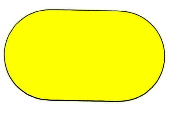
Figure 1: (Color online) Photographs through an optical microscope of some micro-lasers used in this paper. The in-plane scale is about 100 $\mu$m.

Dielectric resonators are widely used in photonics for fundamental research chang and practical applications matsko . Furthermore their wavelength range is not limited to optics and cover other electromagnetic domains like microwaves micro-ondes or Tera-Hertz waves preu . Here we consider quasi-2D organic micro-lasers since they proved to be quite efficient to test trace formulae lebental ; lebental-matsko .

The cavities were etched by electron-beam lithography into a polymethylmethacrylate (PMMA) layer doped with a laser dye spincasted on a silica on silicon wafer. This technology offers appreciable versatility in terms of shapes, while ensuring a small roughness and a good quality for the corners with a resolution better than a tenth of wavelength (see Fig. 6.5 in lebental-matsko ). Some photographs of the cavities studied in this paper are shown in Fig. 1. The fabrication process is relatively fast and reproducible. At the end, the cavity thickness is about 600 nm, while the in-plane scale is of the order of a few dozens of microns, which allows to apply the effective index approximation and therefore to consider these cavities as 2D resonators.

The chosen cavity was uniformly pumped from above at room temperature and atmosphere with a frequency-double pulsed Nd:YAG laser (30 or 700 ps) and its emission, integrated over 30 pump pulses, was collected sideways in its plane with a spectrometer (Acton SpectraPro 2500i) coupled to a cooled CCD camera (Pixis100 Princeton Instruments). The spectral range of the emitted light depends on the dye laser. Here, for DCM, it is centered around 600 nm and so the $kl$ parameter varies from 500 to 1000. Consequently this experimental system is working far away within the semi-classical regime while its coherence properties are ensured by lasing.

The laser emission is mostly TE polarised gozhyk , but for the features which are compared here with theory and numerics, there is not any predicted difference between the TE and TM cases. Among the resonator shapes studied in this paper, the pump polarisation plays a prominent role only for the square where it will be further developed. For the other shapes, it will not be mentioned.

As this paper is focusing on spectral features, we will consider only the emission spectra which, by default, were registered in the direction of maximal emission (i.e. parallel to the sides for square and pentagon djellali , parallel to the shortest axis for the rectangle djellali , and at an angle depending on the shape parameter for stadiums lebental2 ). Moreover in order to be closed enough to the theoretical case of a passive resonator, the cavities were pumped just above the laser threshold. Mode (and orbit) competition is then reduced.

The typical laser spectrum is made of one or several combs of peaks connected (in a crude approximation) with certain periodic orbits. As shown in lebental the geometrical lengths of the underlying periodic orbits can be inferred from the Fourier transform of the experimental spectrum, which is an equivalent of the length density $d(l)$. For instance, for a Fabry-Perot resonator of width $a$, the geometrical length of the single periodic orbit is $L=2a$ and the dephasing after a loop should be a multiple of $2\pi$: $knL=2\pi m$ with $m\in\mathbb{N}^{\star}$. Then the spacing between the comb peaks verifies $\Delta k=2\pi/nL$, leading to a periodic comb pattern and a Fourier transform of the spectrum peaking at $nL$. With our experimental set-up, the precision on the geometrical length $L$ reaches 3 $\%$ after taking duly account of the dispersion due to the effective index and the absorption of the laser dye. So the refractive index which should be used to interpret the Fourier transform is 1.64 for these actual experiments (it is different from the bulk refractive index 1.54 and the effective refractive index 1.50) lebental .

III Regular shapes

This section deals with square, rectangle, and elliptic dielectric cavities, which can be called ’regular’ cases since their closed counterparts (billiard problems) are integrable. To our knowledge no analytical solution has been proposed so far for these cavity shapes in the open case. Nevertheless, their dielectric spectrum shows some characteristic features specific to integrable systems.

The only example of 2D integrable dielectric cavity is the circular one (see e.g. dubertrand ). Therefore its resonances are organized in regular branches labeled by well defined quantum numbers. For the above mentioned ’regular’ cavities with relatively small refractive index it appears that the resonances still follow similar branch structure (see Figs. 3, 6, 9, 14). This is surprising as these dielectric problems are not integrable and strictly speaking there is no conserved quantum number. This unusual regularity can be described by the superscar approximation proposed in lebental . The detailed discussion of the modified superscar model and its application to these problems will be given elsewhere Eugene_square .

III.1 The square cavity

The simplest example of regular cavities is the dielectric square where the inside billiard problem is straightforward. For instance, for Dirichlet boundary conditions, the eigenenergies and eigenfunctions are the following:

$$k_{p,m}^{2} = \frac{\pi^{2}}{a^{2}}(p^{2}+m^{2})\ ,$$

$$\psi_{p,m}(x,y) = \frac{2}{a}\sin\left(\frac{p\pi x}{a}\right)\sin\left(\frac{m\pi y}{a}\right)\ ,$$

where $a$ is the side length and $p$ and $m$ are two positive integers. The outer scattering problem even with the Dirichlet boundary conditions is more difficult as it corresponds to a pseudo-integrable problem (see e.g. pseudoint ) and no explicit analytical solution exists barbara .

III.1.1 Numerics

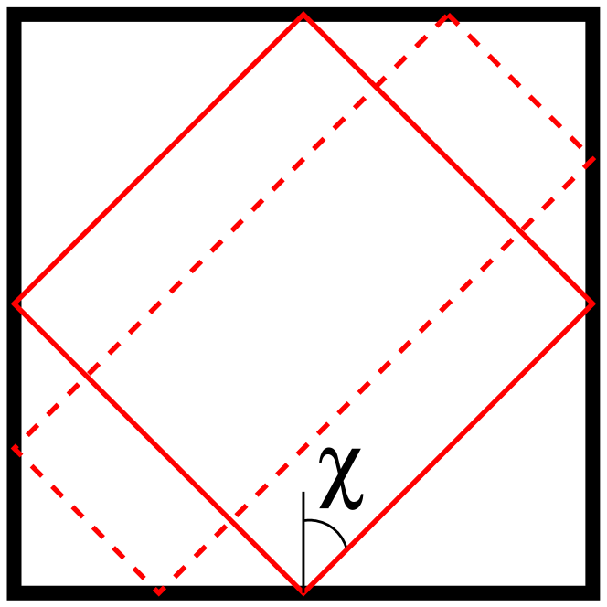
(a)

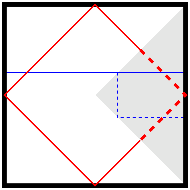
(b)

Figure 2: (a) Two representations of the same diamond periodic orbit. Definition of the incident angle $\chi$. (b) The dashed part corresponds to the fundamental domain used for numerical simulations. The Fabry-Perot and diamond periodic orbits are drawn, as well as their restriction to the fundamental domain (dotted lines).

The solutions of the square dielectric problem can be divided into four symmetry classes corresponding to wave functions odd $(-)$ or even $(+)$ with respect to the diagonals $y=x$ and $y=-x$. For instance, the notation $(-+)$ means that the wave function is odd with respect to the diagonal $y=x$ and even with respect to the other. Each symmetry class reduces to a quarter of a square (dashed part in Fig. 2b) with Dirichlet, $(-)$, or Neumann, $(+)$, boundary conditions along the diagonals. The $(-+)$ and $(+-)$ symmetry classes are equivalent. Fig. 3 shows the resonance spectrum for all symmetry classes and $n=1.5$. Fig. 4 displays some typical quasi-stationary states for the $(--)$ symmetry class from different parts of the spectrum. Notice highly unusual regularity of the spectrum and wave functions for this shape.

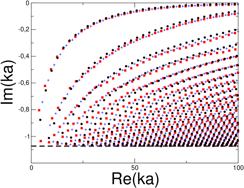
Figure 3: (Color online) Resonance spectrum for the dielectric square with $n=1.5$. The crosses, squares, and circles correspond respectively to $(-+)$, $(++)$, and $(--)$ symmetry classes. The position of the horizontal dashed line is given by (13).

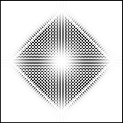
(a)

(b)

(c)

Figure 4: Wave functions for the dielectric square with $n=1.5$ and $(--)$ symmetry class. (a), (b), and (c) correspond to $ka=98.36-0.0071\,\mathrm{i}$, $ka=98.78-1.061\,\mathrm{i}$, and $ka=98.96-0.998\,\mathrm{i}$. Greyscale, black representing maximal values of $|\psi|^{2}$.

As for the case of the circular cavity (see e.g. dubertrand ), the imaginary part of the dielectric square resonances is bounded by the losses $\gamma_{max}$ of the periodic orbit with the highest losses, which is here the Fabry-Perot indicated in Fig. 2b with

$$\gamma_{max}=\frac{1}{n}\ln\left(\frac{n-1}{n+1}\right)\Big{|}_{n=1.5}\simeq-1.073$$ (13)

The counting function $N(k)$ gives the mean number of resonances with a real part less than $k$ in the strip defined by (4). The Weyl-type formula (6) estimates its growth when $k\to\infty$. We checked this prediction for different values of the refractive index and each symmetry class. For $n=1.5$ the results of the numerical fit to the data computed from the spectrum in Fig. 3 are the following

$$(--)\,\,N_{fit}(k) = \frac{n^{2}}{16\pi}(ka)^{2}-0.0866\,ka-0.0456,$$

$$(++)\,\,N_{fit}(k) = \frac{n^{2}}{16\pi}(ka)^{2}+0.2489\,ka-1.737,$$

$$(-+)\,\,N_{fit}(k) = \frac{n^{2}}{16\pi}(ka)^{2}+0.0806\,ka-2.012.$$

Here we fixed the coefficient of the quadratic term and fitted the linear and constant terms from the numerical data.

The predictions of (7) which take into account the Dirichlet or Neumann boundary conditions on two of the sides of the fundamental domain are given by the following expressions calculated for $n=1.5$

$$(--)\,\,\alpha^{th}= \dfrac{\tilde{r}(n)-n\sqrt{2}}{4\pi}\Big{|}_{n=1.5} \simeq-0.0872,$$

$$(++)\,\,\alpha^{th}= \dfrac{\tilde{r}(n)+n\sqrt{2}}{4\pi}\Big{|}_{n=1.5} \simeq 0.2504,$$

$$(-+)\,\,\alpha^{th}= \dfrac{\tilde{r}(n)}{4\pi}\Big{|}_{n=1.5} \simeq 0.0816.$$

The predicted values are in good agreement with our numerical calculations. More precisely, each residue (the difference between $N(k)$ and $N_{fit}(k)$) oscillates around zero as evidenced in Fig. 5.

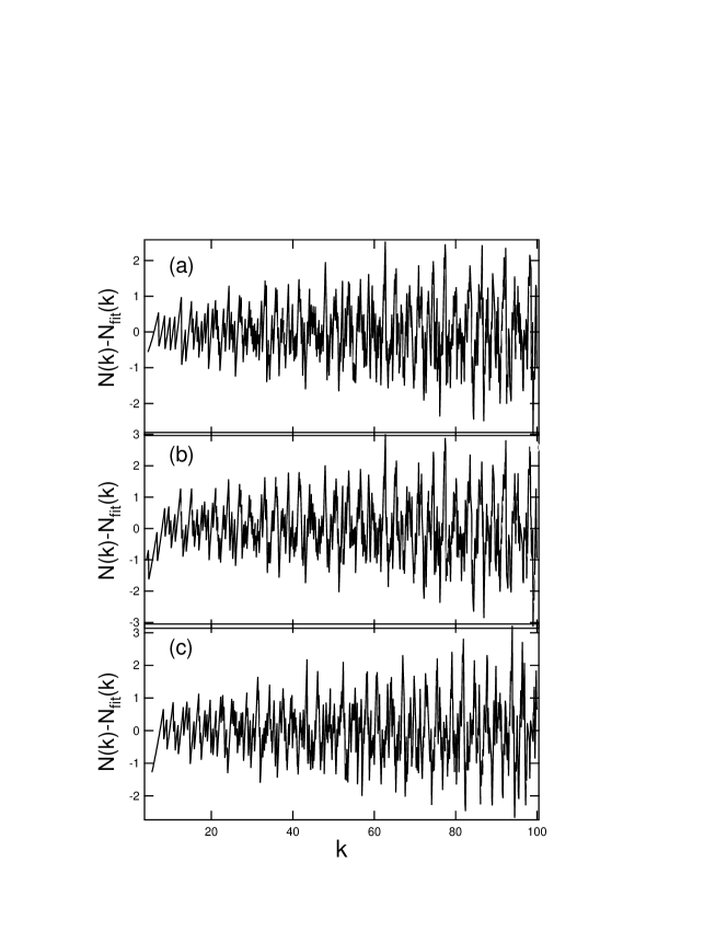
Figure 5: Residue $N(k)-N_{fit}(k)$ for the dielectric square ($a=1$) with $n=1.5$ and different symmetry classes : (a) $(--)$, (b) $(++)$, and (c) $(-+)$.

To ensure the efficiency of formula (6) we calculated the spectrum also for $n=1.35$ with $(--)$ symmetry class, see Fig 6. The quadratic fit for the counting function gives now

$$N_{fit}(k)=\frac{n^{2}}{16\pi}(ka)^{2}-0.0709\,ka-2.052$$

to be compared with:

$$\alpha^{th}=\dfrac{\tilde{r}(n)-n\sqrt{2}}{4\pi}\Big{|}_{n=1.35}\simeq-0.0713.$$

The residue stays also close to zero (see insert in Fig. 6).
In all investigated examples, the agreement between prediction and numerics is better than 2% for the linear term.

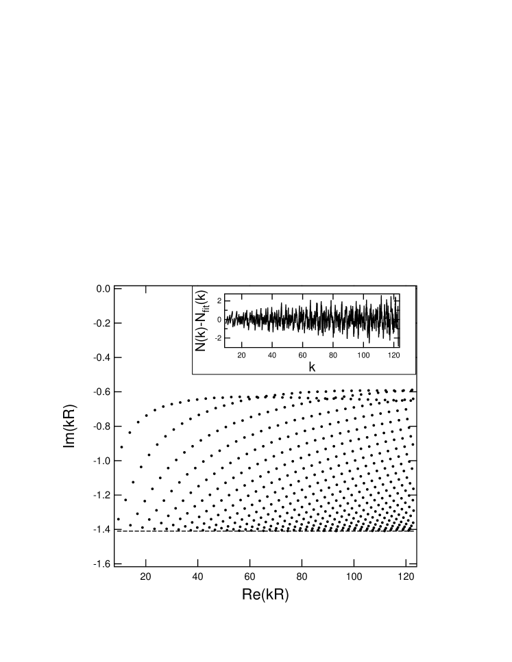
Figure 6: Resonance spectrum for the dielectric square with $n=1.35$ and $(--)$ symmetry class. The positions of the horizontal dashed lines are given by (13). Insert: $N(k)-N_{fit}(k)$ with $a=1$.

The oscillatory part of the trace formula is checked as well. In the square, periodic orbits form families. Thus their weighting is predicted by (11), which implies that the spectrum is dominated by the diamond periodic orbit (see Fig. 2a). Actually the weighting coefficient of this orbit is calculated as follows: it covers the whole cavity (${\cal A}_{\textrm{diamond}}=a^{2}$), its length is short (${\cal L}_{\textrm{diamond}}=2a\sqrt{2}$), and for $n>\sqrt{2}$ there is no refractive loss ($|R_{diamond}|=1$) in the deep semiclassical limit $k\to\infty$. For illustration, it is worth comparing with the $c_{p}$ coefficient of the Fabry-Perot periodic orbit : ${\cal A}_{\mathrm{FP}}=a^{2}$, ${\cal L}_{\mathrm{FP}}=2a$, and $R_{\mathrm{FP}}=[(n-1)/(n+1)]^{2}$. Then for $n=1.5$, $|c_{FP}/c_{diamond}|\simeq 0.05$ mainly due to the prominent influence of refractive losses.

The agreement with numerical simulations is checked via the length density of the dielectric square which is computed from the numerical spectrum using (12). The results are plotted in Fig. 7. The length density is highly peaked at $l=a\sqrt{2}$ and at its harmonics ($l_{m}=ma\sqrt{2}$, with $m\in\mathbb{N}^{\star}$). Only half of the diamond orbit length appears, since the length density is calculated for a single symmetry class and Fig. 2b shows that the diamond periodic orbit is twice shorter if restricted to the dashed area. If the length density had been performed with the four symmetry classes, it would have been peaked at the full diamond length ($2a\sqrt{2}$) and at its harmonics. The same appears with experiments as shown below.

The agreement between numerics and predictions from trace formula (11) is quite good as well when comparing the ratios of the harmonics. Actually these harmonics can be identified as repetitions of the diamond periodic orbit (${\cal L}=m{\cal L}_{\textrm{diamond}}$) and thus formula (11) predicts that the $|c_{p}|^{2}$ should decrease like $1/m$. This prediction is shown by crosses in Fig. 7. From numerics, we received harmonics a little bit smaller than predicted which is natural as the Fresnel reflection coefficient (10) does not take into account correctly a leakage through a dielectric interface of finite length.

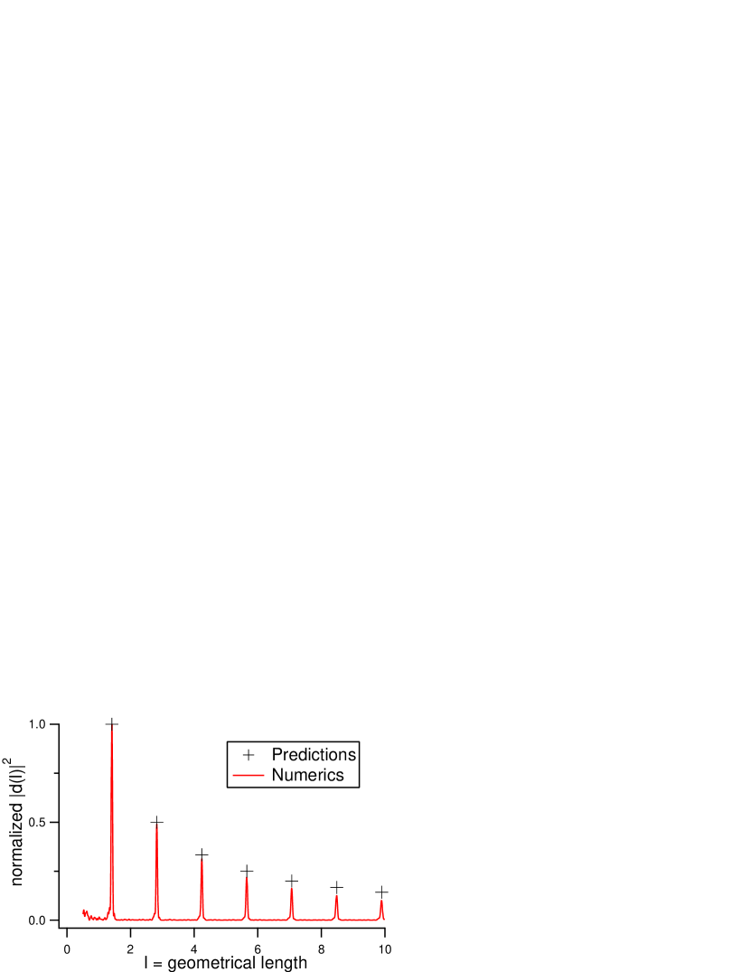
Figure 7: Comparison of $|d(l)|^{2}$ calculated from the numerical data of the dielectric square for $(--)$ symmetry class and $n=1.5$ (continuous line), and predictions from trace formula (crosses) considering the $m^{th}$ repetitions of half the diamond periodic orbit ($l=ma\sqrt{2}$) with a coefficient $|d(l)|^{2}\propto 1/m$.

III.1.2 Experiments

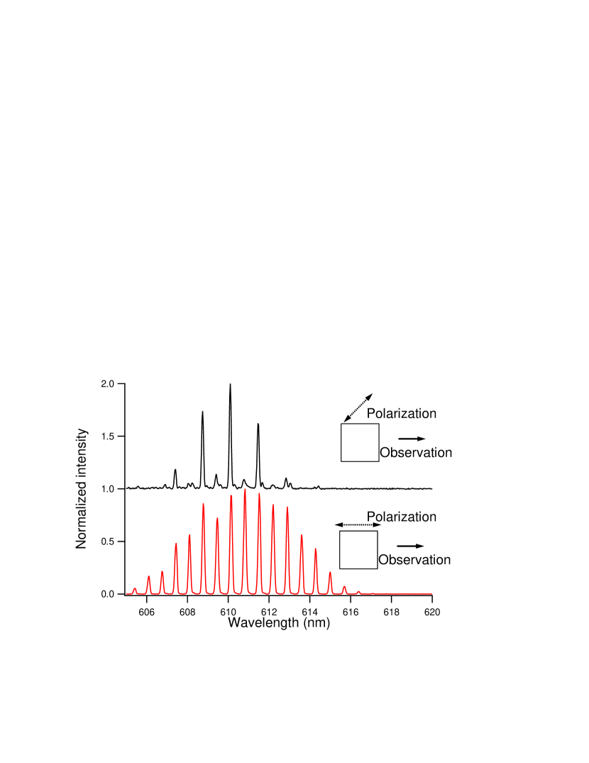
(a)

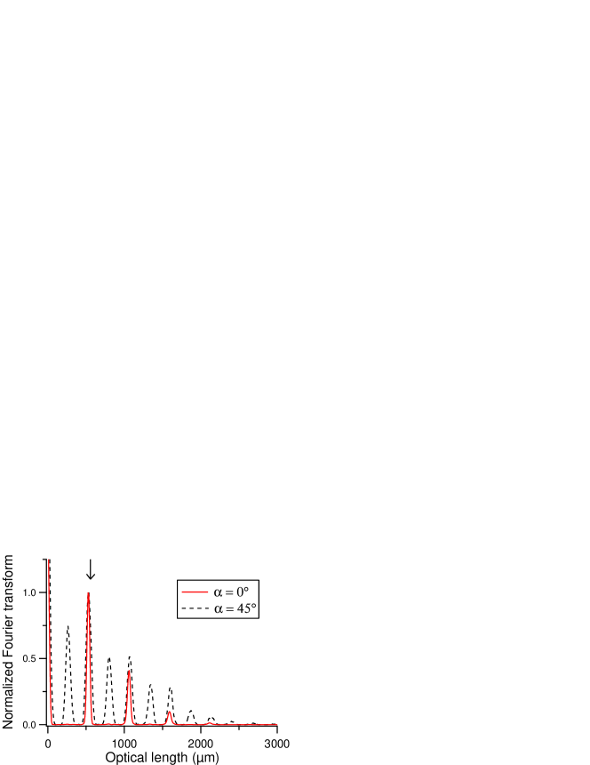
(b)

Figure 8: (Color online) (a) Experimental spectra from a square micro-laser with $a=120\,\mu$m. Top: $\alpha=45^{\circ}$, bottom: $\alpha=0^{\circ}$. (b) Fourier transform of the spectra in (a). The arrow indicates the predicted optical length of the diamond periodic orbit: $2\sqrt{2}a\,n$.

The prevalence of the diamond periodic orbit was already experimentally demonstrated with organic micro-lasers lebental and micro-wave cavities bittner . Here we would like to stress that sometimes the experimental spectrum reveals half the diamond periodic orbit instead of the full one due to a selection of symmetry classes. This phenomenon is illustrated in Fig. 8a using the pump polarization as a control parameter. Actually the DCM molecule (the laser dye) is more or less ’rod-like’ and thus conserves (in a way) the memory of the pump polarization which can be monitored at will without modifying other parameters. A study of the pump polarization influence will be published elsewhere gozhyk .

The Fourier transforms of the spectra in Fig. 8a are plotted in Fig. 8b. Let us call $\alpha$ the angle between the pump polarization (which lies in the plane of the layer) and the direction of observation. For $\alpha=0^{\circ}$, the first harmonic of the Fourier transform is peaked at the diamond optical length. But for $\alpha=45^{\circ}$, only one peak out of two appears in the spectrum, therefore the Fourier transform peaks at half the diamond optical length. It could be noted that the second harmonic (at the actual diamond length) is slightly higher than the first one. This is due to the presence of a residual comb visible in the spectrum (Fig. 8a top).

In this section, we have shown that the spectral properties of the dielectric square (density of states, resonance losses, laser spectra) are controlled in a first approximation by classical features and symmetry classes. For low refractive indices (what we studied), the diamond periodic orbit plays a prominent role.

III.2 The dielectric rectangle

We repeat the same steps as in the previous Section but for a rectangular cavity so as to monitor eventual changes when breaking the square symmetry. Let us call $\rho=L/l$ the ratio between the larger and smaller sides. We will focus on the case $\rho=2$.

III.2.1 Numerics

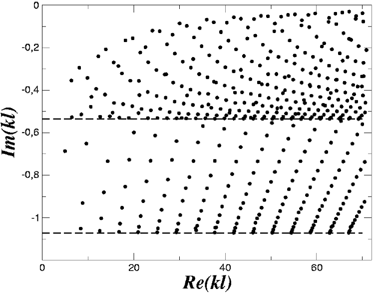
Figure 9: Resonance spectrum of the dielectric rectangle with $\rho=2$, $(++)$ symmetry class, and n=1.5. The positions of the horizontal lines are given by (14) and (15).

We restrict ourselves to the $(++)$ symmetry class with respect to the perpendicular bisectors of the sides (see dashed area in Fig. 11b). Fig. 9 shows the resonance spectrum for this case. The lower bound $\gamma_{max}$ of the imaginary parts of the resonances is related to the lifetime of the classical orbit bouncing off perpendicularly the longest side of the rectangle:

$$\gamma_{max}=\frac{1}{n}\ln\left(\frac{n-1}{n+1}\right)$$ (14)

Another horizontal line is plotted in Fig. 9, which corresponds to the lifetime of the orbit bouncing off perpendicularly the smallest side of the rectangle:

$$\gamma_{2}=\frac{1}{\rho n}\ln\left(\frac{n-1}{n+1}\right)$$ (15)

As for the square cavity, prediction (6) is checked. The best quadratic fit of the counting function $N(k)$ computed numerically from data of Fig. 9 is (with $n=1.5$):

$$N_{fit}(k)=n^{2}\frac{\rho}{16\pi}(kl)^{2}+0.2894\,kl-3.7346\ .$$ (16)

The prediction for the linear term is:

$$\alpha^{th}=\frac{\tilde{r}(n)+n}{8\pi}(1+\rho)\Big{|}_{n=1.5,\rho=2}\simeq 0.3014$$ (17)

which shows a good agreement. The difference between the numerically computed $N(k)$ and its best quadratic fit (16) is shown in Fig. 10.

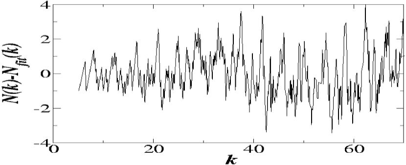
Figure 10: Residue $N(k)-N_{fit}(k)$ for the dielectric rectangle with $\rho=2$, $l=1$, $(++)$ symmetry class, and $n=1.5$.

The length density $d(l)$ defined by (12) is shown in Fig. 11a, and is peaked at the lengths of the double diamond orbit and the stretched diamond orbit (both displayed in Fig 11b).

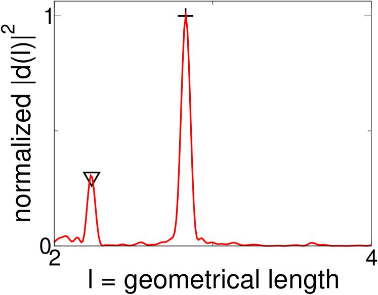
(a)

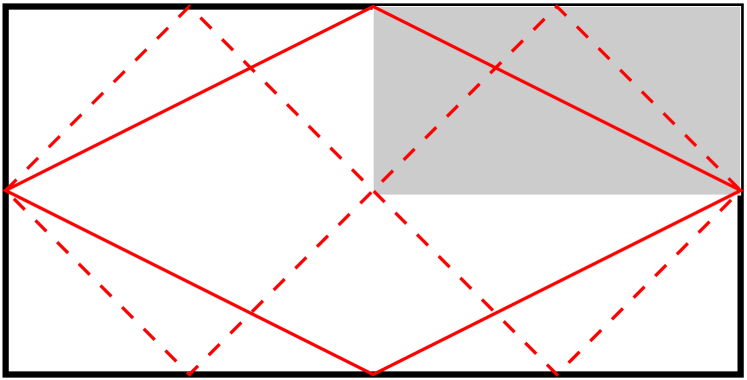
(b)

Figure 11: (a) Length density for a dielectric rectangle calculated from the spectrum in Fig. 9. The expected position of the double diamond (resp. the stretched diamond) is indicated by a cross (resp. a triangle). (b) Main periodic orbits contributing to the resonance spectrum: double diamond (dashed line) and stretched diamond (continuous line). The dashed area corresponds to the fundamental domain.

Eventually some wave functions associated to resonances from different parts of the spectrum are shown in Fig 12.

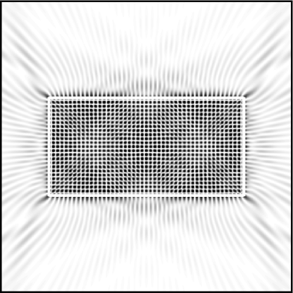
(a)

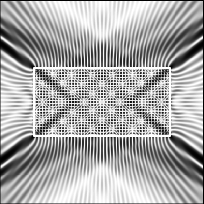
(b)

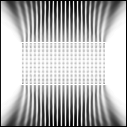
(c)

Figure 12: Quasi-stationary states for the dielectric rectangle, $n=1.5$, $(++)$ symmetry class. (a) $kl=70.04-.038\,\mathrm{i}$, (b) $kl=70.26-.33\,\mathrm{i}$. (c) $kl=70.45-.92\,\mathrm{i}$. Greyscale, black representing maximal values of $|\psi|^{2}$.

III.2.2 Experiments

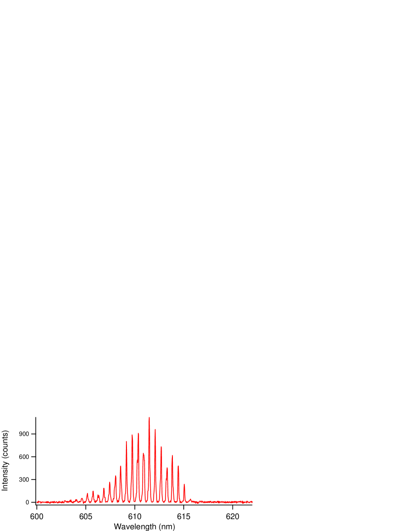
(a)

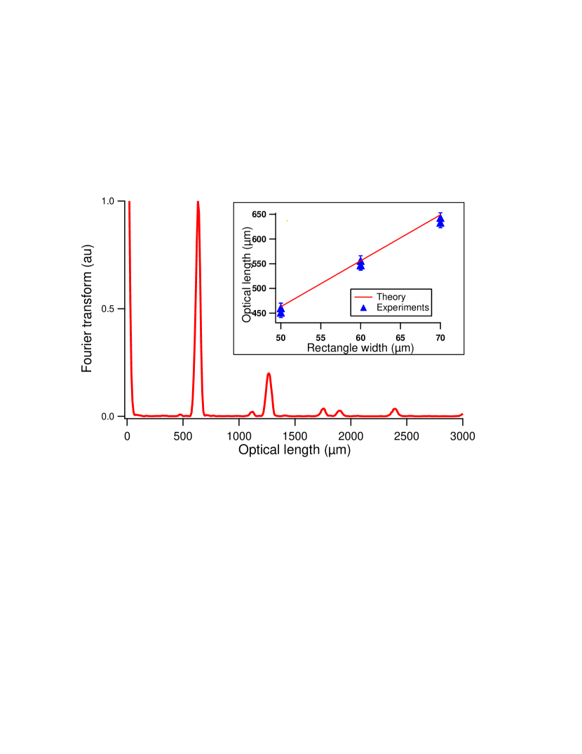
(b)

Figure 13: (Color online) (a) Experimental spectrum of a rectangle microlaser with $\rho=2$ and $l=70\,\mu$m. (b) Fourier transform of the spectrum in (a). Insert: Comparison between the optical lengths inferred from experiments and those expected for the double-diamond for different cavity sizes.

Fig. 13a presents a typical experimental spectrum from a rectangular microlaser with $\rho=2$. Its Fourier transform plotted in Fig. 13b is peaked at the length of the double diamond periodic orbit (see insert), in agreement with numerics and predictions. This experimental observation is very robust whatever the parameter being used: direction of emission, pump intensity, and pump polarization. For illustration, a comparison between the measured and expected optical lengths is presented in insert of Fig. 13b for various cavity sizes. For completeness, it should be noticed that the Fabry-Perot along the longest axis appears if observed in its specific direction and pumped with a favorable polarization.

III.3 The dielectric ellipse

The ellipse can also be considered as a ’regular shape’, since the interior billiard problem is separable bill_ell . Let us call $b$ (resp. $a$) half the length of the minor (resp. major) axis. Here we consider only the ratio $\rho\equiv a/b=2$, however the computations for other $\rho$ values give similar results. Here we will restrict ourselves to the $(--)$ symmetry class, i.e. the function vanishes along both symmetry axis of the ellipse.

III.3.1 Numerics

Fig. 14 shows the resonance spectrum for $\rho=2$. As for the square cavity, it looks quite regular while the problem is not separable. Similarly, the imaginary parts of the resonances are bounded by the losses of the Fabry-Perot periodic orbit (along the minor axis):

$$\quad\gamma_{max}=\frac{1}{2n}\ln\left(\frac{n-1}{n+1}\right)$$ (18)

Figure 14: Resonance spectrum for the dielectric ellipse with $\rho=2$, $(--)$ symmetry class, and $n=1.5$. The position of the horizontal dashed line is given by (18).

Figure 15: $N(k)-N_{fit}(k)$ for the dielectric ellipse ($b=1$) with $\rho=2$ and $(--)$ symmetry class.

Formula (6) for the counting function is checked with the same protocol as before. The residue between numerics and fit is plotted in Fig. 15 and oscillates around zero. Moreover the linear term of the regression

$$\alpha^{fit}=-0.0866$$

agrees well with the prediction:

$$\alpha^{th}=\frac{\tilde{r}(n)\rho E(e)-n(1+\rho)}{4\pi}\Big{|}_{n=1.5,\rho=2}\simeq-0.0872$$

where $E(z)$ is the complete elliptic integral:

$$E(z)=\int_{0}^{\pi/2}\sqrt{1-z^{2}\sin(t)^{2}}\mathrm{d}t\ ,$$ (19)

and $e=\sqrt{1-(b/a)^{2}}$ is the eccentricity of the ellipse.

The oscillatory part will be postponed to a future publication. We already note that the wave functions display in general two kinds of behavior for the wave inside the cavity: either “whispering gallery modes” or “bouncing ball modes” - like as is (rigorously) the case for the elliptic billiard. Fig. 16 presents examples of such wave functions, which correspond to resonances from different parts of the spectrum.

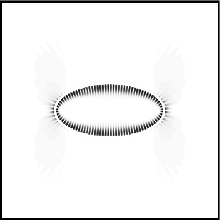
(a)

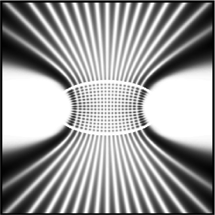
(b)

Figure 16: Wave functions for the ellipse with $\rho=2$, $n=1.5$ and $(--)$ symmetry. (a) Whispering gallery mode, $kb=22.00-0.02\,\mathrm{i}$. (b) Bouncing ball mode, $kb=22.30-0.36\,\mathrm{i}$. Greyscale, black representing maximal values of $|\psi|^{2}$.

III.3.2 Experiments

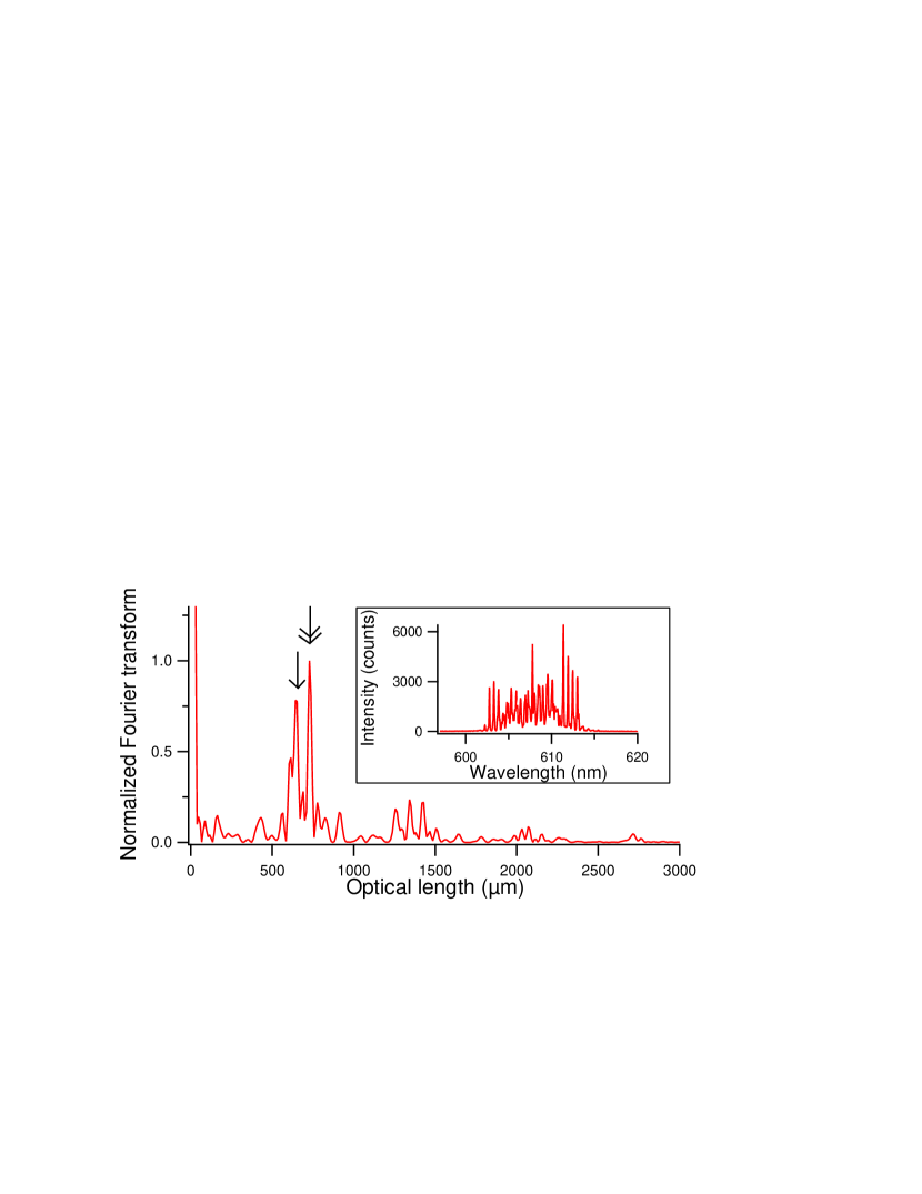
Figure 17: Fourier transform of the spectrum in insert. The arrows indicate the predicted optical length of periodic orbits: single arrow for the Fabry-Perot along the major axis $4a\,n$ and double arrow for the rectangle $4bn\sqrt{1+\rho^{2}}$. Insert: Experimental spectrum from an elliptical micro-laser with $\rho=a/b=2$ and $b=50\,\mu$m registered in the direction parallel to the major axis.

Experiments provide similar insights onto the dominant resonance features. The insert in Fig. 17 shows a typical spectrum from an elliptical micro-laser with $\rho=2$, while its Fourier transform is plotted in the main window. Its first harmonics presents two main peaks with positions corresponding quite well to the optical lengths of two periodic orbits: the rectangle and the Fabry-Perot along the major axis. The deviation is less than 3 %, which is the experimental inaccuracy. It should be noted that for $\rho=2$ the length of the Fabry-Perot along the major axis is equivalent to the second repetition of the Fabry-Perot along the minor axis, also called bouncing ball.

IV Pseudo-integrable system: the dielectric pentagon

Similar studies were performed for the dielectric pentagon and hexagon, which are particularly interesting systems since they contain diffracting angles: $m\pi/n$ with $m,n$ co-prime and $m>1$. Following Richens and Berry pseudoint these systems are called pseudo-integrable, since their classical flow is confined to a surface as for integrable systems but because its genus is bigger than 1 they cannot be classically integrable.

Here we only consider the dielectric pentagon, though every conclusion also applies to the hexagon mutatis mutandis. Below we present the results for the $(--)$ symmetry class, which means that the associated wave functions vanish along each symmetry axis of the polygon. $R$ stands for the radius of the outer circle of the pentagon and $a=2R\sin(\pi/5)$ for its side length.

IV.1 Numerics

(a)

(b)

(c)

(d)

Figure 18: (a) Resonance spectrum for the dielectric pentagon with $(--)$ symmetry and $n=1.5$. The position of the horizontal dashed line is given by (20). (b) $N(k)-N_{fit}(k)$ calculated from the numerical spectrum in (a) with $R=1$. (c) A part of the periodic orbit with the shortest lifetime. (d) A representation of the periodic orbit in (c).

Fig. 18a shows the resonance spectrum of a dielectric pentagon for $(--)$ symmetry and $n=1.5$. Again the imaginary part of the resonances is bounded and this lower bound $\gamma_{max}$ can be estimated from the refractive losses of the periodic orbit drawn in Fig. 18c and d which presents the highest losses (shortest lifetime):

$$\gamma_{max}=\frac{2}{nl}\ln R_{TM}\left(\frac{\pi}{10}\right)\Big{|}_{n=1.5}\simeq-0.630$$ (20)

where $l=2R\left(\sin(2\pi/5)+\sin(\pi/5)\right)$.

Several wave functions are displayed in Fig. 19. It is important to stress the existence of different types of resonances. The ones with low losses are related to ’whispering gallery-like’ modes, see Fig. 19a. In lebental , this observation was used to build a superscar approximation of these resonances. Notice the more complex pattern in (b) for this wave function corresponding to $kR$ with rather large imaginary part, and the scarring by the orbit in Fig. 18d for the wave function in Fig. 19c.

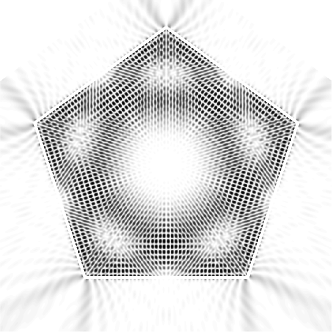
(a)

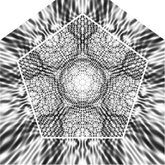
(b)

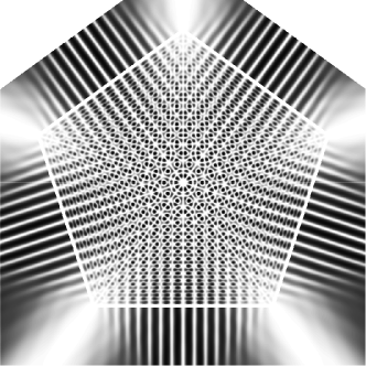
(c)

Figure 19: Wave functions of the dielectric pentagon with $(--)$ symmetry and $n=1.5$. (a) $kR=91.35-0.038\,\mathrm{i}$, (b) $kR=89.06-0.453\,\mathrm{i}$, and (c) $kR=92.56-0.628\,\mathrm{i}$. Greyscale, black representing maximal values of $|\psi|^{2}$.

The Weyl law (6) is checked as above by fitting the counting function $N(k)$ which gives:

$$N_{fit}(k)=\frac{n^{2}\sin(2\pi/5)}{16\pi}(kR)^{2}-0.1681\,kR+0.1077\ ,$$

in good agreement with the prediction for the linear term:

$$\alpha^{th}=\frac{\tilde{r}(n)\sin(\pi/5)-n\,[1+\cos(\pi/5)]}{4\pi}\Big{|}_{n=1.5}\simeq-0.1680$$

Moreover the residue $N(k)-N_{fit}(k)$ oscillates around zero as expected (see Fig. 18b).

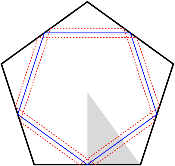
(a)

(b)

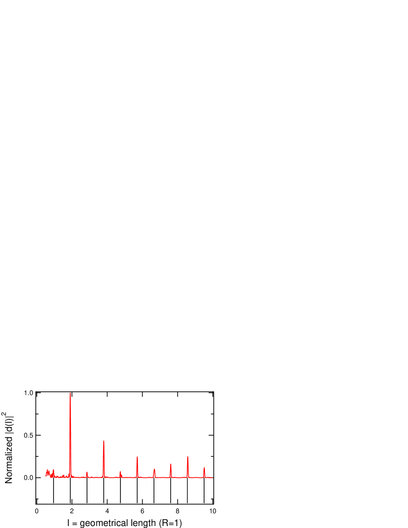
(c)

Figure 20: (Color online) (a) ’single pentagon’ periodic orbit in solid line and ’double pentagon’ periodic orbit in dotted line. The dashed area indicates the fundamental domain used for simulations. (b) A representation of the double pentagon periodic orbit. (c) Length density for the dielectric pentagon calculated from the numerical data plotted in Fig. 18a. The vertical lines in the bottom part of the graph indicate the repetitions of the single pentagon orbit.

The length density plotted in Fig. 20c evidences that a few periodic orbits mostly contributes to the oscillatory part of the trace formula. First the density of orbit length is peaked at a length corresponding to the ’double pentagon’ periodic orbit, which is depicted in Fig. 20a and b. This orbit is confined by total internal reflection for our value of the refractive index and lives in family contrary to the isolated ’single pentagon’ orbit. The length of the single pentagon periodic orbit, once folded in the fundamental domain shown in Fig. 20a, is $l=R\sin(2\pi/5)$. The length of the double pentagon periodic orbit is twice longer. The vertical lines in Fig. 20b indicate the theoretical lengths of the $m^{th}$ repetition of the single pentagon periodic orbit: $l_{m}=m\,l$. As expected, the length density is mostly peaked at the $l_{m}$ positions with even $m$.

a)

b)

Figure 21: Diffracting orbits in the pentagonal cavity.
(a) $l_{a}=R\sqrt{130+22\sqrt{5}}/2$, $7l/l_{a}\approx.995$.
(b) $l_{b}=R\sqrt{210+38\sqrt{5}}/2$, $9l/l_{b}\approx.997$.

Second, it is worth noting that the amplitude of the peaks does not clearly decay as for the square in Fig. 7. For $m=7$ for instance, the peak amplitude is unexpectedly high for a repetition of a given orbit. This happens when the length $l_{m}$ is close to the length of a diffracting orbit. Here, the repetitions $m=7$ and $m=9$ are in fact of similar lengths than the orbits illustrated in Fig. 21. The treatment of such diffracting correction (see a similar discussion in olivier for billiards) is beyond the scope of this paper as it requires the local exact solution of the diffracted field by a dielectric wedge.

IV.2 Experiments

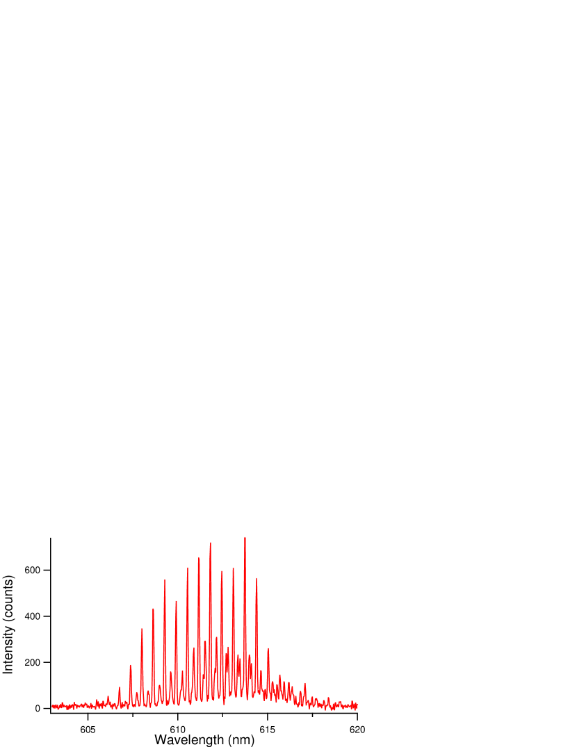
(a)

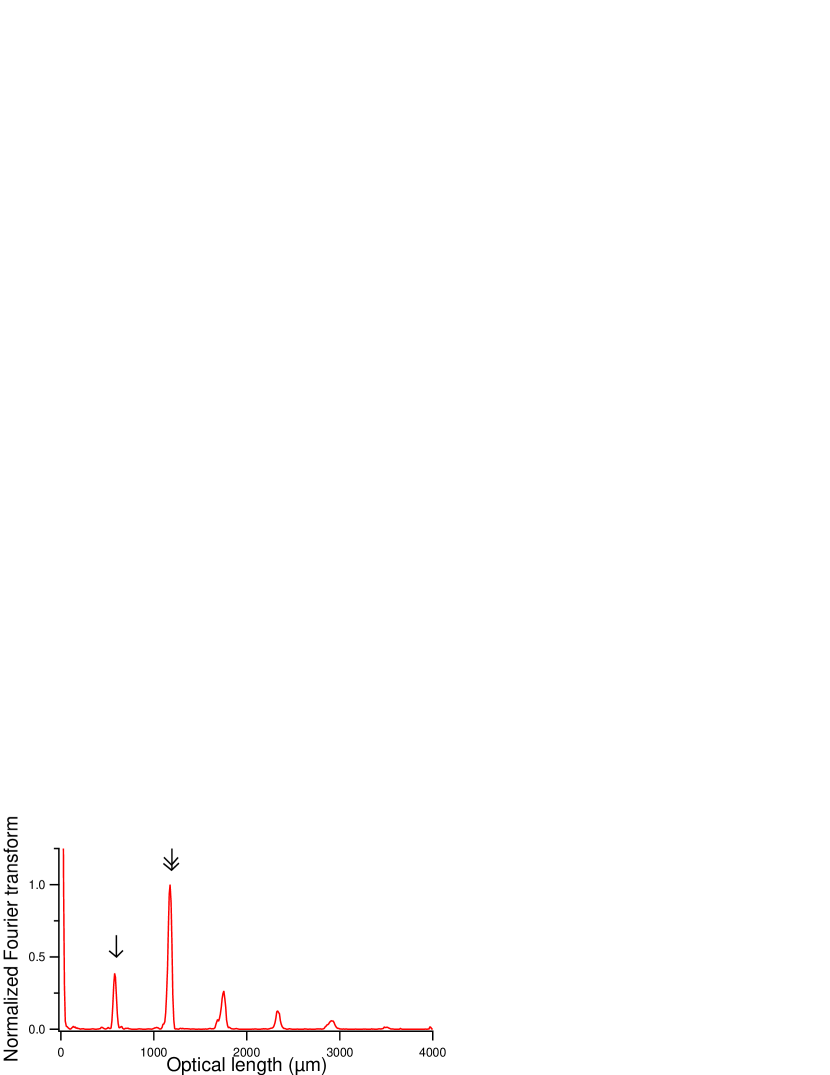
(b)

Figure 22: (a) Experimental spectrum from a pentagonal micro-laser with $a=90\,\mu$m. (b) Fourier transform of the spectrum in (a). The single (resp. double) arrow indicates the expected position of the single (resp. double) pentagon periodic orbit.

A typical experimental spectrum from a pentagonal micro-laser is plotted in Fig. 22a. Its Fourier transform presented in Fig. 22b is mostly peaked at the length of the double pentagon periodic orbit. The single pentagon is visible as well, which can be directly noticed on the spectrum made of two combs of different amplitudes. In lebental , we reported an experimental spectrum from a pentagonal micro-laser where both combs had similar amplitudes and therefore its Fourier transform did not present any peak at the length of the single pentagon. The parameters which control the relative amplitudes of the combs have not been identified yet, but it is clear that the etching quality is a key point.

V Chaotic dielectric cavities

Eventually we applied the same ideas to an archetypal chaotic cavity, the Bunimovich stadium, which is made of a rectangle between two half circles (see Fig. 23b for notations), and investigated various deformation defined by the parameter $\rho=L/R$.

V.1 Numerics

For simplicity we only consider the $(--)$ symmetry class, which means that the associated wave functions vanish along both symmetry axis of the stadium. The resonance spectrum for $\rho=1$ is shown in Fig. 23a. As for the other cavities, the imaginary part of the resonances is bounded and its lower bound $\gamma_{max}$ can be estimated from the refractive losses of the periodic orbit which presents the highest losses, i.e. the Fabry-Perot along the small axis (also called bouncing ball orbit):

$$\gamma_{max}=\frac{1}{2n}\ln\left(\frac{n-1}{n+1}\right)$$ (21)

Again, some wave-functions are presented in Fig. 24, representative of different parts of the spectrum.

(a)

(b)

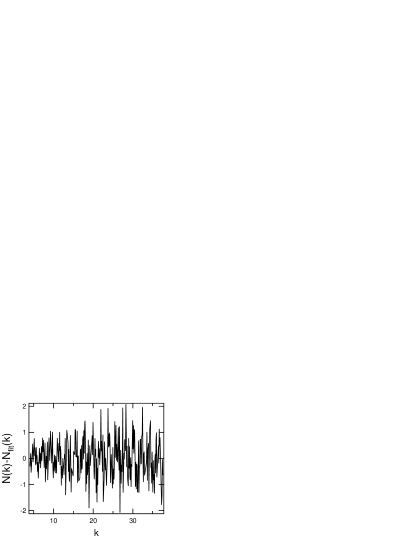
(c)

Figure 23: (a) Resonance spectrum for the dielectric stadium with $\rho=1$, $(--)$ symmetry class, and $n=1.5$. The position of the horizontal dashed line is given by (21). (b) Notations for the Bunimovich stadium. (c) $N(k)-N_{fit}(k)$ calculated from the numerical simulations in (a) with $R=1$.

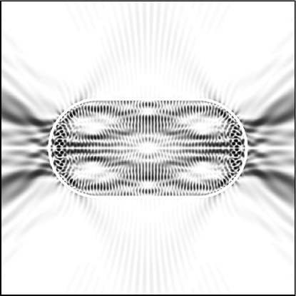
(a)

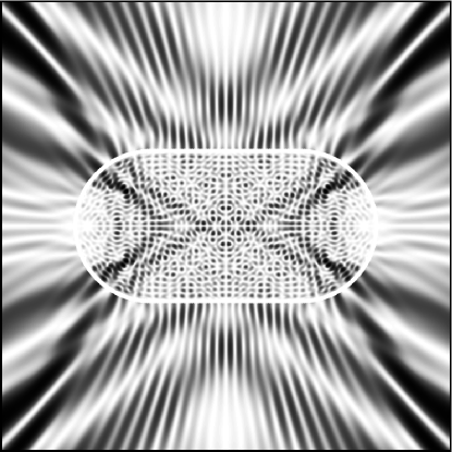
(b)

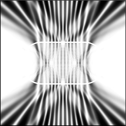
(c)

Figure 24: Wave functions of the dielectric stadium with $\rho=1$, $(--)$ symmetry class, and $n=1.5$. (a) $kR=34.48-0.11\,\mathrm{i}$. (b) $kR=34.55-0.31\,\mathrm{i}$. (c) $kR=34.48-0.45\,\mathrm{i}$. Greyscale, black representing maximal values of $|\psi|^{2}$.

The counting function $N(k)$ was computed from the numerical data shown in Fig. 23a and the best fit gives:

$$N_{fit}(k)=\frac{n^{2}}{4\pi}\left(\rho+\frac{\pi}{4}\right)(kR)^{2}-0.145\,kR-4.042\ ,$$ (22)

to be compared with the prediction (7) for the linear term:

$$\alpha^{th} = \frac{1}{4\pi}\left[\tilde{r}(n)\Big{(}\rho+\frac{\pi}{2}\Big{)}-n\,(2+\rho)\right]\Big{|}_{n=1.5,\rho=1}$$ (23)

$$\simeq -.148\ .$$

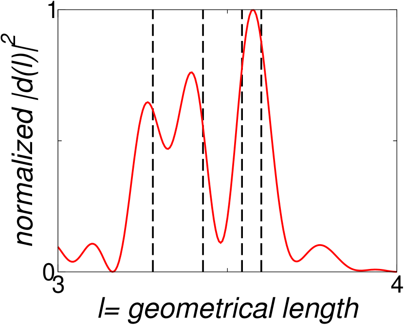
(a)

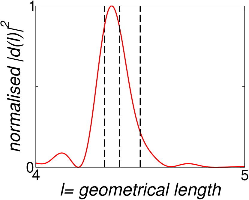
(b)

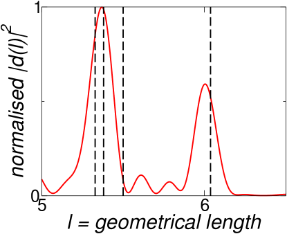
(c)

Figure 25: Length densities calculated from numerical spectra for dielectric stadiums with $(--)$ symmetry class and $n=1.5$. (a) $\rho=0.3$. (b) $\rho=0.75$. (c) $\rho=1.25$. The vertical dotted lines indicate the expected positions of periodic orbits (numbering according to Fig. 26).

The oscillatory part of the trace formula is also checked, plotting the length densities calculated from numerical spectra for several shape ratios $\rho$. The curves presented in Fig. 25 are peaked at different positions which could be assigned to periodic orbits. To predict which periodic orbits should mainly contribute to the length density, we calculated their weighting coefficient from formula (9). The considered orbits are drawn in Fig. 26, their geometrical length is plotted in Fig. 27, and their coefficient (amplitude) versus $\rho$ in Fig. 28a. Note that orbits $5$ and $6$ obey geometrical constraints such as they do not exist for $\rho<1$.

Figure 26: Some periodic orbits of the stadium.

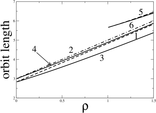
Figure 27: Geometrical length of the periodic orbits plotted in Fig. 26. Numbering according to Fig. 26.

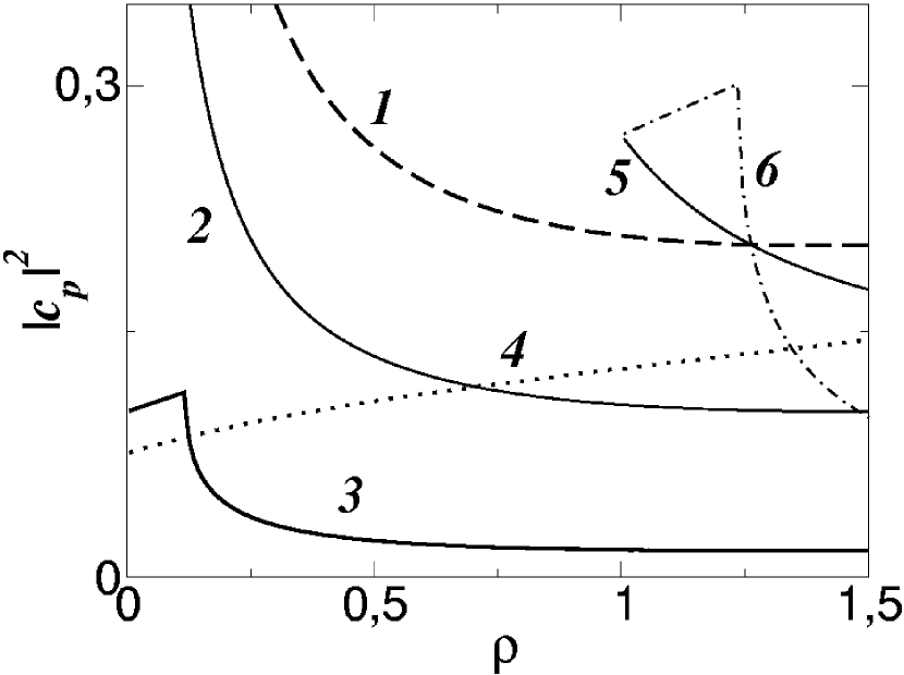
(a)

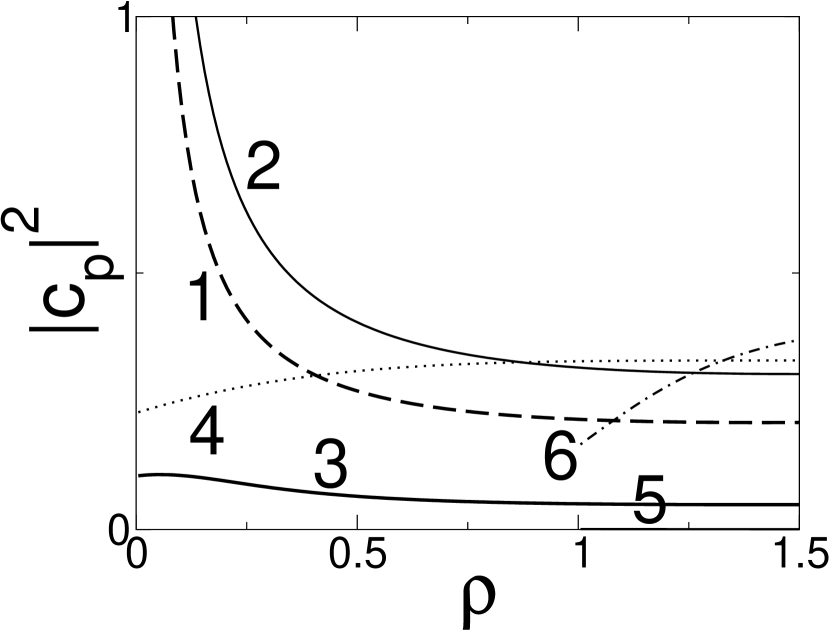
(b)

Figure 28: Amplitude of the orbits listed in Tab. 26 for the $(--)$ symmetry class following formula (9) (a) Semiclassical regime (i.e. no size effect taken into account). (b) Idem with curvature correction calculated for $kR=25$.

The length densities are calculated from the numerical spectra on a finite number of resonances (finite range of Re($kR$)), thus some finite size effects do play a role and must be taken into account evaluating the amplitudes of the periodic orbits. One of the main effect here comes from the curvature correction in the reflection coefficient. If the dielectric boundary is curved enough compared to the wavelength then there is a quite important correction to the standard Fresnel coefficients marthenn . We use the following formula to take into account the curvature correction:

$$R^{(c)}_{TM}=\frac{\sqrt{n^{2}-\dfrac{m^{2}}{x^{2}}}+\mathrm{i}\dfrac{H^{(1)\prime}_{m}}{H^{(1)}_{m}}(x)}{\sqrt{n^{2}-\dfrac{m^{2}}{x^{2}}}-\mathrm{i}\dfrac{H^{(1)\prime}_{m}}{H^{(1)}_{m}}(x)}$$ (24)

where $x=kR$ and $m=nx\cos\chi$. The Fresnel coefficient for a straight interface (10) is recovered for large $kR$, see Fig. 29. In Fig. 28b, the amplitudes of the periodic orbits are plotted taking into account this curvature correction. Notice the important differences with Fig. 28a.

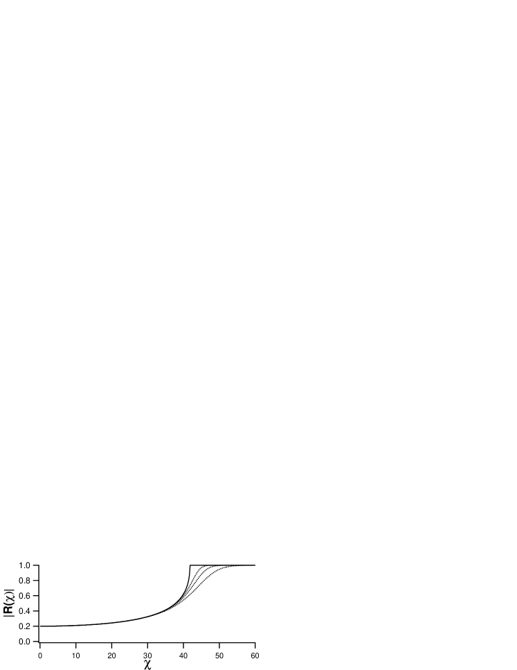
Figure 29: Modulus of the TM reflection coefficient as a function of the incidence angle (in degrees). Full line: Fresnel coefficient (10) for a straight boundary. Dotted lines: (24) for $kR=100,50,25$.

Using Fig. 28b we can give a quantitative estimate of the periodic orbits which mostly contribute to the length density. For $\rho=0.3$ (Fig. 25a), the length density is peaked around the orbits 3 ($l\simeq 3.28$) and 1 ($l\simeq 3.43$), and orbits 2 and 4 with respective length $l\simeq 3.6$ and $l\simeq 3.54$ cannot be separated. For $\rho=0.75$ (Fig. 25b), the orbits $1$ and $4$ with respective length $l\simeq 4.33$ and $l\simeq 4.40$ interfere. The line at $l\simeq 4.5$ stands for orbit $2$. Eventually for $\rho=1.25$ (Fig. 25c), the two orbits 1 and 4 ($l\simeq 5.33$ and $l\simeq 5.38$) interfere. Again we drew a line for orbit 2 at $l\simeq 5.5$. A peak can also be seen for orbit 6 ($l\simeq 6.04$). From these examples it appears that the agreement between theory and numerics is qualitatively good.

V.2 Experiments

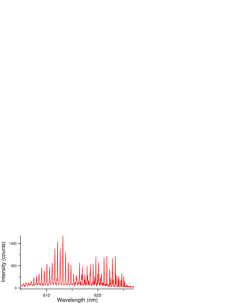
Figure 30: Experimental spectrum of a stadium micro-laser with $\rho=0.75$ and $R=50\,\mu m$. Its Fourier transform is plotted in Fig. 31b.

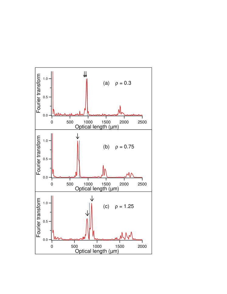
Figure 31: Normalized Fourier transform of experimental spectra from stadium micro-lasers with (a) $R=80\,\mu m$, (b) $R=50\,\mu m$, and (c) $R=45\,\mu m$. The vertical line corresponds to the position of the perimeter. The arrows indicate the expected positions of some orbits, for comparison: (a) orbits 1 and 2, (b) orbit 1, and (c) orbits 1 and 5 (numbering according to Fig. 26).

Spectra were recorded for the shape ratios used in numerical simulations and for various $R$ (see djellali2 for $\rho=0.5$). A typical experimental spectrum from an organic micro-stadium is plotted in Fig. 30 and typical Fourier transforms in Fig. 31. They look similar to those of the shapes studied in the previous sections. However the main difficulty to face when studying stadiums is the large number of orbits with close lengths. Would it be numerically or experimentally, it is thus difficult to assign peaks in the length density. Then, to check formula (9) against experiments, it was decided to compare the positions of the peaks to the length of the perimeter. Actually some crossing orbits like orbits 5 and 6 are longer than the perimeter and, due to geometrical constraints, do not exist for $\rho<1$. Moreover according to Fig. 28a, which corresponds to the semi-classical limit and so to experimental conditions, their amplitudes (9) are the highest when they appear. So we expect Fourier transforms peaked at positions shorter than the perimeter for $\rho<1$ and longer for $\rho\gtrsim 1$, and this is evidenced in Fig. 31.

VI Conclusion

In this paper we have shown numerical and experimental results concerning the trace formula for dielectric cavities. For convex cavities and TM polarization the resonance spectrum can be divided into two subsets. One of them, the Feschbach (inner) resonances which are relevant for experiments, is statistically well described by classical features: the periodic orbit with the shortest lifetime for the lower bound of the wave number imaginary parts, the Weyl’s law for the counting function, and the weighting coefficients of periodic orbits for the length density. The formulæ we derived, based on standard expressions used in quantum chaos and adapted to dielectric resonators, give an accurate description of these spectral properties.

Those formulæ have been checked for various resonator shapes. For ”regular shape” (i.e. the analogous billiard problem is separable) and for small index of refraction, the resonance spectrum presents a branch structure as if the dielectric problem was separable. When the corresponding billiard problem is not integrable, the usual Weyl’s law still occurs. The oscillating part can be also explained by taking into account the shortest periodic orbits. In the chaotic case the correspondence is however more difficult to claim quantitatively as finite size effects play a quite important role because of periodic orbits with close lengths.

The main result of the paper is the demonstration that dielectric cavities widely used in optics and photonics can be well described using generalizations of techniques from quantum chaos.

This study raises many open problems and we would like to mention some of them. The formulæ checked here gave accurate predictions for TM polarization. For TE polarization, due to the existence of the Brewster angle where the reflection coefficient vanishes dettmann , the situation is less clear and requires further investigations. The next step should be to treat carefully the diffraction on dielectric wedges, which is still an open problem burge . A related question is to improve the accuracy of the standard effective index theory, since the separation into TE and TM polarizations is precisely based on this 2D approximation. Experimental data (i.e. real 3D systems) indeed revealed departures from this model gozhyk ; bittner . These questions are related to the wave functions (see e.g. lebental ) and far field patterns, which are also of great interest, especially for applications.

Appendix A Weyl’s law

The Appendix deals with the derivation of formula (6) using an alternative method than in bogomolny . Start from the definition of the Green function $G$:

$$(\Delta_{\vec{x}}+n(\vec{x}\,)^{2}k^{2})\,G(\vec{x},\vec{y}\,)=\delta(\vec{x}-\vec{y}\,)$$ (25)

where $n(\vec{x}\,)$ is equal to $n$ (resp. $1$) when $\vec{x}$ is inside (resp. outside) the dielectric cavity. Moreover, for TM modes, $G(\vec{x},\vec{y}\,)$ and its normal derivative are continuous along the boundary of the domain. Taking the trace of it gives the density of states through the Krein formula (see bogomolny and references therein):

$$d_{all}(E)-d_{0}(E)=$$

$$- \frac{1}{\pi}\int\mathrm{Im}\ \left[n(\vec{x}\,)^{2}G(\vec{x},\vec{x}\,)-G_{0}(\vec{x},\vec{x}\,)\right]\mathrm{d}\vec{x}$$

where the integral runs over the whole 2D plane. $d_{0}(E)$ is the density of states of the free space and $G_{0}(\vec{x},\vec{y}\,)$ stands for the Green function of a free particle in the plane:

$$G_{0}(\vec{x},\vec{y}\,)=\frac{1}{4\mathrm{i}}\,H_{0}^{(1)}(k\left|\vec{x}-\vec{y}\,\right|)$$ (27)

$$=\frac{1}{4\pi\mathrm{i}}\int_{-\infty}^{+\infty}\frac{e^{\mathrm{i}p(x_{1}-y_{1})}}{\sqrt{k^{2}-p^{2}}}e^{\mathrm{i}\sqrt{k^{2}-p^{2}}\,|x_{2}-y_{2}|}\mathrm{d}p$$ (28)

with $\vec{x}=(x_{1},x_{2})$ and $\vec{y}=(y_{1},y_{2})$. $H_{0}^{(1)}(z)$ is the Hankel function of the first kind and Eq. (28) implicitly assumes that $k$ has a small positive imaginary part. It is worth noting that $d_{all}(E)$ is the Krein spectral shift function which is different from the spectral density $d(E)$ discussed in Eq. (5). It will be explained how to get it at the end of this Section.

A.1 Derivation of the first two terms

Figure 32: Plot of $\tilde{r}(n)$.

The leading term of the Weyl’s law is obtained when substituting $G_{0}$ to $G$ in Eq. (A) and using (27):

$$d_{all}(E)-d_{0}(E)\simeq(n^{2}-1)\frac{{\cal A}}{4\pi}$$ (29)

where ${\cal A}$ is the area of the domain filled with the dielectric material.

The first remaining term in (6) comes from the presence of the boundary. Thus it is first necessary to solve the elementary problem of a plane wave reflecting on an infinite straight dielectric boundary, which can be derived through standard methods. Then, using expression (28), the Green function for both $\vec{x}$ and $\vec{y}$ inside the dielectric can be written:

$$G(\vec{x},\vec{y}\,) = \frac{1}{4\pi\mathrm{i}}\int_{-\infty}^{+\infty}\frac{e^{\mathrm{i}p(x_{1}-y_{1})}}{\sqrt{n^{2}k^{2}-p^{2}}}[e^{\mathrm{i}\sqrt{n^{2}k^{2}-p^{2}}\ |x_{2}-y_{2}|}$$ (30)

$$+ R(p)\,e^{\mathrm{i}\sqrt{n^{2}k^{2}-p^{2}}\,|x_{2}+y_{2}|}]\,\mathrm{d}p$$

where $p$ is the tangential component of the momentum and

$$R(p)=\frac{\sqrt{n^{2}k^{2}-p^{2}}-\sqrt{k^{2}-p^{2}}}{\sqrt{n^{2}k^{2}-p^{2}}+\sqrt{k^{2}-p^{2}}}\ .$$ (31)

Similarly one gets the Green function when the arguments are outside the dielectric:

$$G(\vec{x},\vec{y}\,) = \frac{1}{4\pi\mathrm{i}}\int_{-\infty}^{+\infty}\frac{e^{\mathrm{i}p(x_{1}-y_{1})}}{\sqrt{k^{2}-p^{2}}}[e^{\mathrm{i}\sqrt{k^{2}-p^{2}}\ |x_{2}-y_{2}|}$$ (32)

$$- R(p)\,e^{\mathrm{i}\sqrt{k^{2}-p^{2}}\ |x_{2}+y_{2}|}]\,\mathrm{d}p\ .$$

As usual the trace of $G$ is computed using local coordinates. The surface term (29) is recovered from the first terms of (30) and (32), so we focus now on their second terms only. The integration along the boundary gives the length factor ${\cal L}$. For the transverse coordinate, the boundary is approximated locally by its tangent plane, and then (30) and (32) are used. After the convenient Wick rotation $p\to-itk$, the boundary contribution from inside is:

$$\alpha^{(in)}=\dfrac{n^{2}}{8\pi^{2}k}\displaystyle\int_{-\infty}^{+\infty}\frac{R(-\mathrm{i}tk)}{n^{2}+t^{2}}\mathrm{d}t\ .$$ (33)

Similarly from (32) the boundary contribution is:

$$\alpha^{(out)}=-\dfrac{1}{8\pi^{2}k}\displaystyle\int_{-\infty}^{+\infty}\frac{R(-\mathrm{i}tk)}{1+t^{2}}\mathrm{d}t\ .$$ (34)

Putting together (33) and (34) back to (A), one gets the first two terms of the Weyl expansion:

$$d_{all}(E)-d_{0}(E)\simeq(n^{2}-1)\frac{{\cal A}}{4\pi}+\frac{(\tilde{r}(n)-1){\cal L}}{8\pi k}\ ,$$ (35)

where, noting $R(t)$ instead of $R(-\mathrm{i}tk)$:

$$\tilde{r}(n)=1+\frac{n^{2}}{\pi}\int_{-\infty}^{+\infty}\frac{\mathrm{d}t}{t^{2}+n^{2}}R(t)-\frac{1}{\pi}\int_{-\infty}^{+\infty}\frac{\mathrm{d}t}{t^{2}+1}R(t)\ .$$ (36)

$\tilde{r}(n)$ is plotted in Fig. 32.

A.2 From the density of states to the count of Feschbach resonances

As mentioned above, the quantity entering the Krein formula is not exactly the spectral density (5), but they can be related heuristically. The spectral shift function, $d_{all}(E)$ in (A), is related with the determinant of the full $S$-matrix for the scattering on a cavity, while $d(E)$ in (5) is the spectral density of Feschbach (inner) resonances which are poles of this $S$-matrix. In addition to these poles, the determinant of the $S$-matrix may have poles associated with shape resonances (which we do not take into account) and then an additional phase factor $d_{s}(E)$:

$$d_{all}(E)=d(E)+d_{s}(E).$$ (37)

It is natural to assume (and can be checked for dielectric disk) that for all outside structures the corresponding wave functions are almost zero inside the cavity and on its boundary. Therefore the $S$-matrix phase, $d_{s}(E)$, associated with such functions in the leading order is the same as for the outside scattering on the same cavity but with the Dirichlet boundary conditions. The Weyl expansion for such scattering is known (see petkovpopov ; robert2 and references therein):

$$d_{s}(E)-d_{0}(E)\simeq-\frac{{\cal A}}{4\pi}-\frac{{\cal L}}{8\pi k}\ .$$ (38)

Subtracting (38) to (35) gives the desired result for the spectral density, taking into account only Feschbach resonances:

$$d(k)=2kd(E)\simeq n^{2}\frac{{\cal A}k}{2\pi}+\frac{\tilde{r}(n)}{4\pi}\,{\cal L}\ .$$ (39)

Then Eq. (6) is recovered by integration.

References

- (1) K. J. Vahala, Nature 424, 839 (2003)
- (2) A.B. Matsko, Practical applications of microresonators in optics and photonics, CRC Press (2009)
- (3) E. Bogomolny, R. Dubertrand, C. Schmit, Phys. Rev. E, 78, 056202 (2008)
- (4) P. Lax, R. S. Phillips, Scattering Theory, Springer NY (1963)
- (5) V. Petkov, G. Popov, Ann. Inst. Fourier 32, 111 (1982)
- (6) U. Smilansky and I. Ussishkin, J. Phys. A: Math. Gen. 29, 2587 (1996)
- (7) D. Robert, Partial differential equations and mathematical physics, Birkhäuser Boston (1996)
- (8) D. Robert, Helv. Phys. Acta 71, 44 (1998)
- (9) G. Popov, G. Vodev, Comm. in Math. Phys. 207, 411 (1999)
- (10) M. Lebental, N. Djellali, C. Arnaud, J.-S. Lauret, J. Zyss, R. Dubertrand, C. Schmit, E. Bogomolny, Phys. Rev. A, 76, 023830 (2007).
- (11) M. Lebental, E. Bogomolny, and J. Zyss, in Practical applications of microresonators in optics and photonics, A. Matsko, CRC Press (Boca Raton, 2009).
- (12) S. Bittner, B. Dietz, M. Miski-Oglu, Oria Iriarte, A. Richter, F. Schäfer, Phys. Rev. A 80, 023825 (2009).
- (13) J. Sjöstrand and M. Zworski, Acta Math. 183, 191 (1999).
- (14) M. Gutzwiller, Chaos in classical and quantum mechanics, Springer Berlin (1990).
- (15) R. Balian, C. Bloch, Ann. Phys. 60, 401 (1970); Ann. Phys. 64, 271 (1971); Ann. Phys. 69, 76 (1972).
- (16) R. K. Chang et A. J. Campillo eds., Optical processes in microcavities, World Scientific (1996).
- (17) D. Kajfez and P. Guillon, Dielectric resonators, Norwood MA (1986).
- (18) S. Preu, H. G. L. Schwefel, S. Malzer, G. H. Dhler, L. J. Wang, M. Hanson, J. D. Zimmerman, and A. C. Gossard, Optics Express, 16, 7336 (2008).
- (19) I. Gozhyk et al., to be published.
- (20) S. Lozenko, N. Djellali, J. Lautru, I. Gozhyk, D. Bouche, M. Lebental, C. Ulysse, and J. Zyss. Submitted.
- (21) M. Lebental, J.-S. Lauret, J. Zyss, C. Schmit, and E. Bogomolny, Phys. Rev. A75, 033806 (2007).
- (22) R. Dubertrand, E. Bogomolny, N. Djellali, M. Lebental, C. Schmit, Phys. Rev. A 77, 013804 (2008).
- (23) E. Bogomolny et al, to be published
- (24) P. J. Richens & M. V. Berry, Physica D 2, 495 (1981)
- (25) B. Dietz, U. Smilansky, Physica D 86, 34 (1995)
- (26) S. Bittner, E. Bogomolny, B. Dietz, M. Miski-Oglu, P. Iriarte, A. Richter, and F. Schäfer, Phys. Rev. E81, 066215 (2010).
- (27) E. Mathieu, J. Math. Pures et Appl. 13 (in French), 137 (1868)
- (28) E. Bogomolny, O. Giraud, C. Schmit, Comm. in Math. Phys. 222, 327 (2001)
- (29) M. Hentschel, H. Schomerus, Phys. Rev. E 65, 045603 (2002).
- (30) N. Djellali, I. Gozhyk, D. Owens, S. Lozenko, M. Lebental, J. Lautru, C. Ulysse, B. Kippelen, and J. Zyss, Appl. Phys. Lett. 95, 101108 (2009).
- (31) C. P. Dettmann, G. V. Morozov, M. Sieber, H. Waalkens, EPL 87, 34003 (2009).
- (32) R. Burge, X.-C. Yuan, B. Carroll, N. Fisher, T. Hall, G. Lester, N. Taket, and C. Oliver, IEEE Transactions on antennas and propagation, 47, 1515 (1999).