The structure of the $\beta$ Leonis Debris Disk

Abstract

We combine nulling interferometry at 10 $\mu$m using the MMT and Keck Telescopes with spectroscopy, imaging, and photometry from 3 to 100 $\mu$m using Spitzer to study the debris disk around $\beta$ Leo over a broad range of spatial scales, corresponding to radii of 0.1 to $\sim$100 AU. We have also measured the close binary star o Leo with both Keck and MMT interferometers to verify our procedures with these instruments. The $\beta$ Leo debris system has a complex structure: 1.) relatively little material within 1 AU; 2.) an inner component with a color temperature of $\sim$600 K, fitted by a dusty ring from about 2 to 3 AU; and 3.) a second component with a color temperature of $\sim$120 K fitted by a broad dusty emission zone extending from about $\sim$5 AU to $\sim$55 AU. Unlike many other A-type stars with debris disks, $\beta$ Leo lacks a dominant outer belt near 100 AU.

1. Introduction

The IRAS discovery of excess infrared radiation from many stars introduced a powerful new approach to study neighboring planetary systems. The dust that radiates in the infrared in these ”planetary debris systems” is cleared away on timescales much shorter than the lifetime of the host stars, through processes such as radiation pressure and Poynting-Robertson drag. Its presence indicates the existence of larger bodies that replenish it through cascades of collisions (Backman & Paresce, 1993). These bodies may be organized into large circumstellar structures analogous to the asteroid and Kuiper Belts in the Solar System. Like them, this extrasolar debris may be shepherded by the gravity of large planets. Moreover, the dust location is a tracer of the non-gravitational drag and ejection forces, as well as of other effects such as sublimation if the dust approaches the star too closely. The structure of a relatively easily detected planetary debris system therefore reveals clues about the nature of the undetectable planetary system that sustains the debris.

Although readily detected with cryogenic space infrared telescopes (e.g., IRAS, ISO, Spitzer, and Herschel), only a small fraction of debris systems have well-understood structures. The small apertures and long operating wavelengths of these infrared telescopes provide inadequate resolution to resolve the majority of known debris systems well. Scattered light imaging, particularly with HST, can only reach disks of high optical depth (Kalas et al., 2005; Wyatt, 2008). Ground-based imaging in the infrared can provide geometric information such as width, inclination and the presence of rings, warps or asymmetries (e.g., Telesco et al., 2005), but is sensitive only to high-surface-brightness structures. Spectral data can provide information on the chemical composition and temperature of a debris disk; however, it leaves the grain size and distance from the central star poorly determined, since both are derived from the grain optical properties. Combining infrared spectral and imaging data is necessary to decode the information that debris disks can provide about planetary systems.

Different spectral regions preferentially probe different radial zones around the central star. Simple arguments from the Wien Displacement Law and radiative equilibrium show, for example, that 2 $\mu$m measurements should be dominated by dust at $\sim$1500 K, which would lie at several tenths of AUs from a luminous A-type star. Similarly, observations at 10 $\mu$m will preferentially be sensitive to dust at a distance of 2–5 AU, those at 24 $\mu$m will be dominated by structures at 10–20 AU, and measurements at 70 $\mu$m are best suited to probe in the $\sim$100 AU region, which for most debris disks appears to be the outermost zone. A consistent combination of observations over the entire spectral range of 2 to 100 $\mu$m is required to build a reasonably comprehensive model of a debris system. Only a few systems have been modeled in this way, such as Vega (Su et al., 2005; Absil et al., 2006).

In this paper, we report observations of $\beta$ and o Leo with the Keck Interferometer Nuller (KIN), the Bracewell Infrared Nulling Cryostat (BLINC) on the MMT, and with Spitzer. Both KIN and BLINC are operated at 10 µm and trace material close to the star: KIN has a resolution of 0$\farcs$012 and field of view of $\sim$0$\farcs$5, which is complemented by BLINC observations at a resolution of 0$\farcs$2 and a field of view of 1$\farcs$5. Spitzer has a beam of 6″ at 24 µm and 18″ at 70 µm. Together these three facilities can search for extended dust emission from 0$\farcs$01 to $\sim$10″, corresponding to 0.1–100 AU.

We present the observations in Section 2 and general results in Section 3. In Section 4 we discuss and analyze all available data of $\beta$ Leo to set constraints on the circumstellar material. We then build a physical disk model based on these derived properties with assumed grain properties in Section 5, followed by discussion of the results and a conclusion in Section 6 and Section 7.

2. Observations And Data Reductions

2.1. BLINC

Details about the method of nulling interferometry employed by BLINC can be found in the appendix. Briefly, the method involves delaying a beam from one aperture by half a wavelength and then overlapping it with a beam from a second aperture. The destructive interference that results can be arranged to suppress the light coming from the central star, allowing faint, extended emission to be observed. Specifically, BLINC is sensitive between radii of $\sim$0$\farcs$12 and 0$\farcs$8.

Observations were carried out on 2008 March 27 at the 6.5 m MMT, located on Mount Hopkins, AZ. They consisted of taking ten 1-s frames on targets and calibrators with BLINC set to interfere the apertures destructively. These measurements were followed by nodding the telescope 15″ to take ten 1-s background frames. The process was then repeated with BLINC set to interfere the apertures constructively. To maximize observing efficiency, 40-frame sets of destructive images were occasionally taken for $\beta$ and o Leo, since these frames had low signal to noise, while constructive images were skipped. All of the observations reported here used an N-band filter, covering roughly 8 to 13 µm.

Table 1 lists the number of frames taken for each star in both destructive and constructive modes of BLINC, as well as the number of usable frames. We discarded the observed frames when the adaptive optics (AO) system broke lock in the middle of taking a dataset (often due to wind gusts), and when BLINC did not properly set the pathlength difference between beams. In addition, some frames taken at the end of observing $\beta$ and o Leo, as well as all the frames taken on the calibrator star $\alpha$ Boo were adversely affected by weather conditions and were discarded. The results of comparing the weather-affected $\beta$ and o Leo data with the $\alpha$ Boo data are consistent with the data presented here, but with substantially larger error bars.

Table 1Summary of Observations at MMT

Star	Total frames	Total frames	Used frames	Used frames
	destructive	constructive	destructive	constructive
$\beta$ Gem	160	150	79	80
$\beta$ Leo	480	200	260	70
o Leo	720	150	680	120
$\alpha$ Boo	50	50	0	0

2.2. KIN

Observations of $\beta$ Leo and o Leo were obtained with the Keck Interferometer Nuller (KIN) during runs on 2008 February 16–18 and 2008 April 14–16. The 85 m baseline on KIN provides the ability to detect circumstellar material in the N-band at angular separations of a few milliarcseconds from the primary star, within the KIN field of view defined as an elliptical Gaussian with FWHM of 0$\farcs$5x0$\farcs$44 (Colavita et al., 2009). Thus, the observations taken by KIN are spatially complementary to the shorter baseline of BLINC. Each primary aperture at Keck is further divided into two subapertures, with a baseline of 5 m, which are perpendicular to the long baseline. This results in a second, broader set of interference fringes, perpendicular to the primary fringes, which are modulated to take sky background measurements. A detailed description of this procedure can be found in Koresko et al. (2006).

Each individual observation of a star consists of about 10 minutes of data collection, made up of several hundred null/peak (i.e., destructive/constructive) measurements. These measurements are averaged to produce a final value for the null. Observations of science objects are alternated with observations of calibrator stars. Table 2 lists the observations taken at KIN. Further details of the KIN design, observation procedures, and data reduction can be found in Colavita et al. (2006), Koresko et al. (2006), Colavita et al. (2008) and Colavita et al. (2009)).

Table 2Summary of Observations at KIN

Target	Date	Start Time	# Scans	Total duration
		(UT)		(s)
$\beta$ Leo	18 Feb 2008	10:27	3	1827
$\beta$ Leo	16 Apr 2008	6:36	3	1827
o Leo	16 Feb 2008	10:51	2	1351
o Leo	17 Feb 2008	10:40	3	2157
o Leo	14 Apr 2008	7:10	3	1867

2.3. Spitzer

Table 3Spitzer Observations of $\beta$ Leo

AOR Key	Date	Instrument	Module	Integration
3921152	2004 May 17	IRAC Mapping	Ch 1-4	26.8 s $\times$ 5 dithers
18010112	2006 Dec 30	IRAC Mapping	Ch 2,4	26.8 s $\times$ 5 dithers
4929793	2005 Jan 3	IRS Staring	SL, LL	6 s $\times$ 1 cycle
14500608	2006 Jun 8	MIPS Photometry	24 µm, 5 cluster pos.	3 s $\times$ 4 cycles
14496768	2006 Jan 14	MIPS Photometry	24 µm, 5 cluster pos.	3 s $\times$ 4 cycles
9807616	2004 Jun 1	MIPS Photometry	70 µm, default scale	10 s $\times$ 3 cycles
4313856	2004 Jun 1	MIPS Photometry	70 µm, fine scale	3 s $\times$ 1 cycle
			(9 cluster pos.)
8935936	2004 Jun 1	MIPS Photometry	160 µm, 9 cluster pos.	3 s $\times$1 cycle
17325056	2006 Jun 12	MIPS SED-mode	1′ chop	10s $\times$10 cycles

$\beta$ Leo was observed using all three instruments on Spitzer : InfraRed Array Camera (IRAC, Fazio et al. 2004), InfraRed Spectrograph (IRS, Houck et al. 2004) and Multiband Imaging Photometer for Spitzer (MIPS, Rieke et al. 2004). Details about the observations are listed in Table 3. The observations at 24 µm were done at two epochs (2006 Jan 13 and 2006 Jun 08) in standard small-field photometry mode with four cycles with 3 s integrations at 5 sub-pixel-offset cluster positions, resulting in a total integration of 902 s on source for each epoch. The 70 µm observations were done in both default- and fine-scale modes on 2004 May 31 with a total on-source integration of 250 s for the default scale and 190 s for the fine scale. The MIPS SED-mode observations were obtained on 2006 Jun 12 with 10 cycles of 10 s integrations and a 1′ chop distance for background subtraction, resulting in a total of 600 s on source. The 160 µm observations were obtained with the original photometry mode with an effective exposure of $\sim$150 s near the source position. All of the MIPS data were processed using the Data Analysis Tool (Gordon et al., 2005) for basic reduction (e.g., dark subtraction, flat fielding/illumination corrections), with additional processing to minimize instrumental artifacts (Engelbracht et al., 2007; Gordon et al., 2007; Lu et al., 2008; Stansberry et al., 2007). After correcting these artifacts in individual exposures, the final mosaics were combined with pixels half the size of the physical pixel scale for photometry measurements. The calibration factors used to transfer the instrumental units to the physical units (mJy) are adopted from Engelbracht et al. (2007) for 24 µm; Gordon et al. (2007) for 70 µm; Lu et al. (2008) for MIPS-SED mode data, and Stansberry et al. (2007) for 160 µm.

The IRS spectral data were processed starting with the Basic Calibrated Data (BCD) products from the SSC IRS pipeline S18.7. To maximize the quality of the final spectrum, we adopted the extraction methods developed by the Formation and Evolution of Protoplanetary Systems (FEPS: Meyer et al. 2006) and Cores to Disks (C2D: Evans et al. 2003) Spitzer legacy science teams, and based in part on the SMART software package (Higdon et al., 2004). Full details of the process are presented in Bouwman et al. (2008) and Swain et al. (2008). Here we briefly summarize the important elements of the extraction technique.

We begin with the droopres intermediate BCD product. Background subtraction is accomplished by subtracting associated pairs of the 2D imaged spectra from the two nodded positions along the slit. This also eliminates stray light contamination and anomalous dark current signatures. Bad pixels were replaced by interpolating the values in the surrounding 8 pixels. A 6.0 pixel fixed-width aperture was used in the extraction. We optimized the position of the extraction aperture for each order by fitting a sinc profile to the collapsed and normalized source profile in the dispersion direction. The irsfringe package was used to remove low-level fringing for wavelengths $>$20 µm.

Our custom extraction relies on relative spectral response functions (RSRFs) derived independently using stars from the FEPS legacy program free of any thermal excess emission (Bouwman et al., 2008; Carpenter et al., 2008). This RSRF assumes that the object is perfectly centered in the slit, but slight order mismatches are evident in the extracted spectra suggesting that the object was not centered. Such an offset can induce a wavelength dependent curvature in the extracted spectra because of the fixed slit size and diffraction-limited PSF. We employed an algorithm developed by J. Bouwman & F. Lahuis (described in Swain et al. 2008) to correct for this offset. This process dramatically reduced the order offsets. However, a small residual offset remains between the SL1 and LL2 modules.

The final absolute flux density calibration is derived by processing the SSC primary IRS calibrators with the exact same algorithms as used for the FEPS stars (Carpenter et al., 2008) and our program star. The uncertainty in the final absolute calibration is estimated to be $\sim$10%.

$\beta$ Leo was observed with IRAC at two epochs: 2004 May 7 (AOR Key 3921152 and 4306176); and 2006 Dec. 30 (AOR Key 18010112). In both the 3921152 and 18010112 datasets, the star was observed in full-frame mode with 30 s frame times and a 5-position small-scale dither pattern, for a total of 134 s integration time on-source in each band. While the 3921152 dataset contains data in all IRAC bands, images only at 4.5 and 8.0 $\mu$m were acquired in 18010112. In the 4306176 dataset, the star was observed in all bands in full frame mode with a 12 s frame time, repeated twice and with no dithers. Due to the much shorter exposure and the absence of dithering (limiting the spatial sampling of the star on the IRAC arrays), we have discarded the 4306176 dataset. For the other two datasets we first created individual mosaics in each band starting from the BCD (pipeline version S18.5.0), using our custom post-BCD software IRACproc (Schuster et al., 2006), which is based on the SSC mosaiker MOPEX.

3. Results

3.1. BLINC

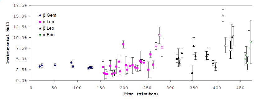
Figure 1.— Instrument nulls of individual datasets for calibrator stars $\beta$ Gem (diamonds) and $\alpha$ Boo (circles) as well as for science stars o Leo (squares) and $\beta$ Leo (triangles) as a function of time. Hollow points indicate sets not used in our analyses due to weather. Error bars are determined by variations of the null within the set.

As an initial test for dataset quality, a 16$\times$20 pixel box centered around the star (which corresponds to 0$\farcs$8$\times$1″ on the sky) is used to calculate the BLINC instrument null. An elongated box is used instead of a circular aperture because the aperture for BLINC is elliptical, making the PSF of a star elliptical as well. The 16$\times$20 pixel box size ensures most (though not necessarily all) of the flux from the system is measured. Figure 1 shows the average null for each set. Since each set contains either 10 or 40 frames, error bars are determined by the deviation of the nulls in individual frames from the average null of the whole set. A filled point is considered good data that is used for further analysis, while a hollow data point is rejected due to weather. Weather-rejected data occurred consistently for all stars when the telescope rotated into a substantial wind. This wind resulted in problems maintaining the telescope’s AO system stability and, consequently, the null.

For the good datasets, the calibration star $\beta$ Gem has only small variations both within a set (as indicated by the small error bars) and from set to set. The fact that $\beta$ Gem has a non-zero null demonstrates the necessity of having calibrator stars: minor movements of the star due to vibrations in the system and sky turbulence result in imperfect suppression (chromatic effects on the null are minimized by a ZnSe corrector in the non-shifted beam path). For the science stars, there is greater variation than is seen for $\beta$ Gem. This is primarily due to the science stars being much dimmer in the N-band, making them more sensitive to changes in background sky brightness. Using weighted means to combine all the good measurements for each star, $\beta$ Gem has an instrumental null of 3.19$\pm$0.09%, o Leo has 3.33$\pm$0.28% and $\beta$ Leo has 4.93$\pm$0.29%. Using the $\beta$ Gem instrumental null as a baseline, we find source nulls of 0.14$\pm$0.30% for o Leo and 1.74$\pm$0.30% for $\beta$ Leo. This indicates that, within errors, o Leo does not have resolved emission, while $\beta$ Leo has resolved emission at 5$\sigma$ significance.

Information pertaining to the variation of the null with respect to separation from the star can be gained by measuring the null within strips of increasing vertical separation from the center of the PSF. Due to the vertically changing transmission pattern of BLINC (illustrated in Figure Aa), such strips are more natural to use than circular annuli. Each dataset has its instrumental null calculated within 16$\times$3 pixel strips. For each separation, all good datasets for a star are combined via weighted means, which also provides the errors. The instrumental nulls for $\beta$ Gem, o Leo and $\beta$ Leo are shown in Figure 2a, while Figure 2b shows the source null for o Leo and $\beta$ Leo. The x-axis is expressed as an angular separation from the center of the system, since 1 pixel has a width of 0$\farcs$054.

In Figure 2a, both $\beta$ Gem and $\beta$ Leo show an increase in the instrumental null beyond $\sim$0$\farcs$5. This is likely caused by residuals from the adaptive optics systems, as well as imperfect beam alignment (both of which are also evident in the fact that the calibrator star has a non-zero null). Data for o Leo only extend to 0$\farcs$4 since beyond this separation, slow variations in sky background became comparable to the brightness of o Leo itself when being imaged destructively. As a result, the destructive signal became lost in the noise.

The source null of o Leo (Figure 2b) does not show evidence (at a 3 $\sigma$ confidence or greater) of any resolved emission within 0$\farcs$4. For $\beta$ Leo, however, an excess null is present out to a separation of at least 0$\farcs$6 (beyond which the error bars become too large to determine whether or not extended emission is present). It must be cautioned that while Figure 2 provides evidence of extended emission, it cannot be straightforwardly interpreted to be evidence for continuous emission from the inner limit of BLINC out to at least 0$\farcs$6: the measured excess is a result of the incoming excess multiplied by the interferometer transmission function and convolved with the PSF of the telescope aperture. Modeling is necessary to interpret the figure, and is presented in section 4.3.2.

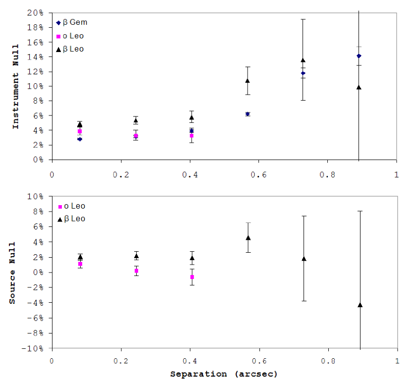
Figure 2.— Strip nulls as a function of separation from the center for $\beta$ Gem (diamonds), o Leo (squares) and $\beta$ Leo (triangles). (a) The instrument null. (b) The calibrator-subtracted source null. Values and errors are determined from weighted means.

3.2. KIN

Table 4 shows the calibrated nulls derived from the KIN observations. The nulls in the table are an average of the observations taken on each night, and are analogous to the ”source nulls” derived for the BLINC data, with both having been calibrated using a calibrator star. The quoted errors are taken to be the larger of the ’external’ error for that date, or the average of the ’formal’ errors for all the scans on that date. The ’formal’ error is defined to be the scatter in the null within a given scan, while the ’external’ error is calculated as the standard deviation among all scans on a given night, divided by the square root of the number of scans (additional information on these errors can be found in Colavita et al. (2009)).

Table 4Calibrated Nulls at KIN

Target	Date	Start Time (UT)	Null (%)	Err. (%)
$\beta$ Leo	18 Feb 2008	10:27	0.9	0.7
$\beta$ Leo	16 Apr 2008	6:36	-0.1	0.3
o Leo	16 Feb 2008	10:51	-0.4	1.0
o Leo	17 Feb 2008	10:40	3.6	0.3
o Leo	14 Apr 2008	7:10	1.7	1.0

3.2.1 $\beta$ Leo

We find that there is no significant nulled flux around $\beta$ Leo, in contrast to the MMT results. Implications of this result are discussed in Section 4.3. The quality of data taken in the 2008 February run was low compared to the data taken in the later run, resulting in larger errors. Due to the relatively low data quality, the 2008 February data were reduced ’manually’ (i.e., taking into account the relatively low percentage of data passing quality gates as well as some non-standard observing procedures), rather than using an automated pipeline. However, it should be noted that the result of both sets of reductions (manual and pipeline) agree within the errors. Furthermore, both the February and April data are consistent and suggest no resolved circumstellar emission within the KIN aperture.

3.2.2 o Leo

For o Leo, two of three sets of observations show evidence for resolved flux. The first set shows a negative null, which is non-physical, though the result is consistent with zero resolved emission within the errors. The last set of data, taken on 14 April, shows a non-zero null; however, large errors result in this detection being only at a level of 1.8 $\sigma$, which we do not consider to be significant. The observations taken on 2008 February 17 yield a detection of resolved emission that can be considered robust. This is in contrast to the MMT results which show no resolved emission. However, interpretation of the KIN resolved emission is more complicated as o Leo is a double-lined spectroscopic binary (Hummel et al., 2001). Detailed modeling (Appendix B) has determined that the resolved flux is consistent with emission from the stellar pair, which has a separation of about 4.5 mas (Hummel et al., 2001). Furthermore, the behavior of the null over time is consistent with the orbital solution calculated by Hummel et al. (2001). If binarity is indeed the source of the excess seen by KIN, this explains why it was not observed by BLINC as well: the separation between the stars is much too small to be detected by BLINC. Additional information on o Leo can be found in the appendix.

3.3. Spitzer Results

The photometry at 24 µm was obtained using aperture photometry on each of the five cluster data sets for both epochs. Two aperture settings were used (small: a radius of 6$\farcs$23 with sky annulus between 19$\farcs$92 and 29$\farcs$88 and an aperture correction of 1.699; large: a radius of 14$\farcs$94 with sky annulus between 29$\farcs$88 and 42$\farcs$33 and an aperture correction of 1.142). Such aperture-corrected MIPS photometry generally agrees to within $\sim$1% for a clean, non-saturated point source. The large aperture gives a total integrated flux density of 1623$\pm$33 mJy (2% error assumed), which is $\sim$2.5% higher than the small one (This behavior is similar to that of the resolved disk of $\gamma$ Oph at 24 µm (Su et al., 2008)). This result suggests $\beta$ Leo is slightly more extended than a true point source at 24 µm. Therefore, we adopt the large aperture result as the final photometry in the 24 µm band.

However, the FWHM measurements of the source at 70 µm are consistent with it being a point source as compared to calibration stars that have a similar brightness at this wavelength. The 70 µm photometry was extracted using PSF fitting, giving a total flux density of 711$\pm$50 mJy (7% error assumed) in the 70 µm band. The MIPS SED-mode data were extracted using an aperture of 5 native pixels ($\sim$50″) in the spatial direction. The final MIPS SED-mode spectrum was further smoothed to match the resolution at the long-wavelength portion of the spectrum (R=15).

The 160 µm observation needs additional attention to eliminate the filter leak contamination. The expected stellar photospheric brightness at 160 µm is $\sim$26 mJy, resulting in a leak strength of $\sim$390 mJy ($\sim$15 times) that is brighter than the expected disk brightness assuming its emission is blackbody-like. Visual inspection of the 160 µm data confirms that the $\beta$ Leo observation was mostly dominated by the ghost image (off position). We used the 160 µm observation (AOR Key 15572992 from PID 52) of Achernar (HD10144, B3Ve) for the leak subtraction as both 160 µm observations were obtained in the same way (dithered cluster position). A constant background value of 7.5 MJy sr^-1 for Achernar and of 10 MJy sr^-1 for beta Leo was taken out in each of the mosaics first. We then scaled the Achernar data by a factor of 0.34 for subtraction, and a faint source appeared in the expected position of $\beta$ Leo after the subtraction. Because the background (most due to instrument artifacts) is not very uniform, the source is only weakly detected. The pixel-to-pixel variation of the observation suggests a point source 1-$\sigma$ sensitivity of 30 mJy in this observation. We placed a 16″ radius aperture at the position of the source to estimate the source brightness. After proper aperture correction (Stansberry et al., 2007), a flux density of 90 mJy is estimated. Achernar is a nearby (42.75 pc; van Leeuwen 2007) fast rotating Be star with a close (0$\farcs$15) companion (Kervella & Domiciano de Souza, 2007). Kervella et al. (2008) estimated the companion has spectral type of A1V-A3V based on the near-infrared colors and contributes 3.3% of the combined photospheric emission. The color-corrected IRAS flux densities are consistent with the expected levels of the photosphere represented by the Kurucz model of $T_{\ast}\sim$15,000 K, $logg$=3.5, and solar metallicity (Kervella et al., 2009), scaled to match the distance of the star and stellar radius of 8.5 $R_{\sun}$. Using the same photospheric model, the expected 160 µm value for Achernar is 68 mJy. Part of Achernar’s photosphere is subtracted off from the $\beta$ Leo data for the leak subtraction. After correcting this, the faint source at the expected $\beta$ Leo position has a flux density of 114 mJy. However, this value is a lower limit due to the uncertainty in scaling the leak subtraction. Varying the scaling by $\pm$10% results in a 30% change in the photometry. Because of the difficulty of leak subtraction and low signal-to-noise of the data, we do not consider the source to be detected at 160 µm. The source brightness is likely within 114–217 mJy. Futhermore, Herschel has measured $\beta$ Leo with PACS at 100 and 160 µm with flux densities of 500$\pm$50 mJy and 230$\pm$46 mJy, respectively (Matthews et al., 2010). We then adopted the Herschel values to constrain the amount of cold dust in the $\beta$ Leo system in later analysis.

Since $\beta$ Leo is saturated in the IRAC observations at all bands, we extracted the photometry based on PSF fitting. We have derived its Vega magnitudes by fitting the unsaturated wings and diffraction spikes with a PSF derived from the observations of bright stars (Vega, Sirius, $\epsilon$ Eridani, Fomalhaut, and $\epsilon$ Indi). The construction of this PSF and the details of the adopted PSF-fitting technique are described in Marengo et al. (2009). The PSF files are available at the SSC web site. We estimated the magnitude uncertainty by bracketing the best fit with over- and under-subtracted fits in which the PSF-subtraction residuals were comparable to the background and sampling noise. The IRAC photometry for $\beta$ Leo based on the epoch 1 data is magnitudes (Vega) of 1.905 $\pm$ 0.011, 1.909 $\pm$ 0.011, 1.875 $\pm$ 0.011, and 1.927 $\pm$ 0.011 for the IRAC [3.6], [4.5], [5.6]. and [8.0] bands, respectively. The data quality in the second epoch is lower than in the first one, so we used it only as a rough confirmation of these results. We converted the PSF-fit magnitudes into fluxes by adopting the zero point (Vega) fluxes listed in the IRAC Data Handbook version 3.0 (2006). The resulting photometry and associated errors are listed in Table 5. The spatial extension of the $\beta$ Leo disk could not be constrained with the IRAC images because of the PSF core saturation. The measured photometry and spectra along with previous measurements from the literature are shown in the spectral energy distribution (SED) in Figure 3.

Table 5Broadband Phometry of $\beta$ Leo

$\lambda_{c}$ [µm]	Star $F_{\nu}$ [Jy]	Total $F_{\nu}$ [Jy]	Error $F_{\nu}$ [Jy]	$\chi$	Fraction [%]	Origin
$[3.6]$	47.967	48.435	1.085	0.4	1.0	IRAC
$[4.5]$	31.083	30.971	0.693	-0.2	-0.4	IRAC
$[5.8]$	19.731	20.450	0.458	1.6	3.6	IRAC
$[8.0]$	10.547	10.759	0.244	0.9	2.0	IRAC
23.675	1.189	1.647	0.033	13.9	38.5	MIPS
25.000	1.066	1.647	0.247	2.4	54.6	IRAS
71.419	0.128	0.743	0.052	11.8	481.6	MIPS

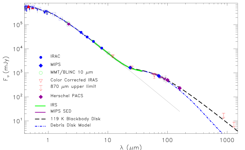
Figure 3.— The SED of the $\beta$ Leo system. Most of the symbols and lines used are shown on the plot except for the optical ground-based photometry (open squares from Johnson system, filled circles from Hipparcos Tycho system, filled triangle from Strömgen system). The 870 µm upper limit (3$\sigma$) is from Holmes et al. (2003).

4. Analyses

In this section, we use the measurements described above to characterize the infrared excess emission of $\beta$ Leo. We first establish the properties of the star, which we use to extrapolate the photospheric output from the near-infrared. This process lets us subtract the photospheric contribution to the mid-infrared measurements to reveal the excess due to circumstellar dust. We then consider the upper limit on the extended emission from the KIN. Finally, we simulate the BLINC data to determine the constraints it places on the disk structure at 10 $\mu$m.

4.1. Stellar Photospheric Emission

To determine the stellar photospheric emission, we fit all available optical to near-infrared photometry (Johnson $UBV$, Strömgen $uvby$ photometry, Hipparcos Tycho $BV$ photometry, 2MASS $JHK_{s}$ photometry) with the synthetic Kurucz model (Castelli & Kurucz, 2003) based on a $\chi^{2}$ goodness of fit test. Because of the star’s proximity, the 2MASS photometry is saturated and unusable. In addition, $\beta$ Leo has been found to have a hot $K$-band (2.14 µm) excess of 2.17$\pm$1.4 Jy (Akeson et al., 2009) ($\sim$2.5% above the photosphere). To overcome these difficulties, we tried to include other ground-based near-infrared photometry. $\beta$ Leo is a primary bright standard in the UKIRT/Mauna Kea System, with m_K = 1.98, $H-K$ = 0.01, and $J-K$ =0.04. Combining all the available data and transforming to the 2MASS system resulted in a $K_{s}$ of 1.93 mag for the photospheric fitting.

A value of $T_{eff}$=8500 K with a total stellar luminosity of 13.44 $L_{\sun}$ integrated over the Kurucz model spectrum at the given distance gives the best $\chi^{2}$ value. This suggests that the stellar radius is 1.7 $R_{\sun}$ using the Stefan-Boltzmann equation. In comparison, Akeson et al. (2009) estimate the stellar radius to be 1.54$\pm$0.021 $R_{\sun}$ based on the long-baseline interferometric observation from CHARA array. Their radius was derived including a fit with an incoherent flux (hot excess), while the early VLTI interferometric observation by Di Folco et al. (2004) derived a much larger radius (1.728$\pm$0.037 $R_{\sun}$) without including the incoherent flux. Additionally, Decin et al. (2003) use various methods to determine a stellar radius in the range of 1.68 – 1.82 $R_{\sun}$ for $\beta$ Leo, consistent with a spectral type of A3V. A stellar radius of 1.5 $R_{\sun}$ is the nominal value for a F0V star with an expected effective temperature of 7300 K, making it too cool to fit the observed photometry for $\beta$ Leo. We do not attempt to solve the mystery of stellar radius for $\beta$ Leo. However, we use 1.7 $R_{\sun}$ as the stellar radius in the thermal models for computing dust temperatures in order to be consistent with the stellar radiation field. (The difference in stellar radius produces a $\sim$22% difference in input stellar luminosity). Using a stellar mass of 2.0 $M_{\sun}$ and the derived stellar luminosity, the blowout size ($a_{bl}$ in radius) is $\sim$3 µm for astronomical silicate grains (Laor & Draine, 1993).

Based on the best-fit Kurucz model, we then estimate the stellar photospheric flux densities at the wavelengths or bands of interest. For MIPS observations, the expected photospheric flux densities are computed based on the monochromatic wavelength of each band, while the expected photospheric fluxes are integrated over the bandpasses for the IRAC observations. The additional 2% errors of the photosphere determination (mostly limited by the K-band photometry accuracy) have been added to the IRAC measurements. The broadband phometry obtained by this work and their corresponding photospheric flux densities are listed in Table 5.

4.2. Infrared Excess around $\beta$ Leo

4.2.1 Near Infrared

The colors of beta Leo in the UKIRT/Mauna Kea System are $H-K$ = 0.01, and $J-K$ = 0.04 with estimated errors of 1%. They agree nearly perfectly with expectations for the spectral type of the star, A3V (e.g., Tokunaga, 2000). The IRAC measurements at [3.6] and [4.5] are also in agreement with those for an A3V star, to within their errors of $\sim$ 1%. Thus, there is no evidence for an excess at the 2.5% level as suggested by the results of Akeson et al. (2009), unless the excess has near infrared colors identical to those for $\beta$ Leo itself. Nevertheless, these photometry results cannot rule out any hot 2 µm excess at the 1% level. New observations obtained with CHARA/FLUOR suggest that the K-band excess around $\beta$ Leo could be smaller than what was reported in Akeson et al. (2009) (O. Absil priv. comm.).

4.2.2 Spitzer Mid- and Far-Infrared Photometry

The expected photospheric contribution in the MIPS 24 µm band is 1190 mJy, indicating that the flux seen at 24 µm is dominated by the star and that the excess emission is 433 mJy (before color correction). However, the flux seen in the 70 µm band is dominated by the excess emission (583 mJy before color correction) compared to the stellar photosphere. This suggests that the dust emitting at MIPS wavelengths has a color temperature of $\sim$120 K. Therefore, color correction factors of 1.055 and 1.054 are applied to the excess emission at 24 and 70 µm, respectively. The infrared excess flux densities are then 457 and 615 mJy in the 24 and 70 µm bands with assumed calibration errors of 2% and 7%, respectively.

At 24 µm, the stellar photosphere was subtracted from the data by scaling an observed point spread function (PSF) to the expected photospheric flux density of $\beta$ Leo and to 1.25 times this value. This over-subtraction technique has been applied to other 24 µm resolved disks like $\gamma$ Oph (Su et al., 2008) and Fomalhaut (Stapelfeldt et al., 2004) to reveal excess emission lying close to the star. The results are shown in Figure 4. The FWHM of the 24 µm image is 5$\farcs$77$\times$5$\farcs$75 before the photospheric subtraction, but is 6$\farcs$88$\times$6$\farcs$61 after the subtraction, which is considerably larger than a typical red PSF (for example, the $\zeta$ Lep disk has a FWHM of 5$\farcs$61$\times$5$\farcs$55, Su et al. 2008). The resolved core emission at 24 µm is best shown in the average radial surface brightness profile (Figure 5). It is evident that the first dark Airy ring (between radii of 5$\farcs$5–7$\farcs$5) in the $\beta$ Leo profile is filled in compared to a true point source, and the profile matches well with that of a point source at larger radii. The position angle of the disk (after photospheric subtraction) is 118° with an error of 3° estimated from two epochs of data. The ratio (1.041) between the semi-major and semi-minor radii in the FWHM suggests the disk is viewed at 20° $\pm$10° , close to face-on (a ratio of 1.011 is expected for a point source while a ratio of $\sim$1.115 is derived from the $\gamma$ Oph disk with inclination of $\sim$50°). The low inclination angle of the disk is consistent with the star being inclined at 21.5° from pole-on (Akeson et al., 2009).

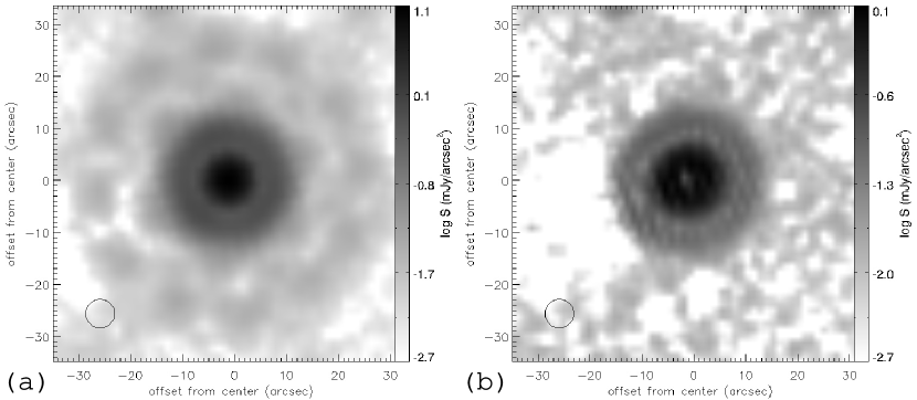
Figure 4.— MIPS 24 µm images of the $\beta$ Leo disk with N up and E toward the left. The nominal beam size (FWHM) is indicated as black circles on the images. The surface brightness scale is to the right of each image. (a) 24 µm image after photospheric subtraction. (b) 24 µm image after over-subtraction of the model stellar photosphere.

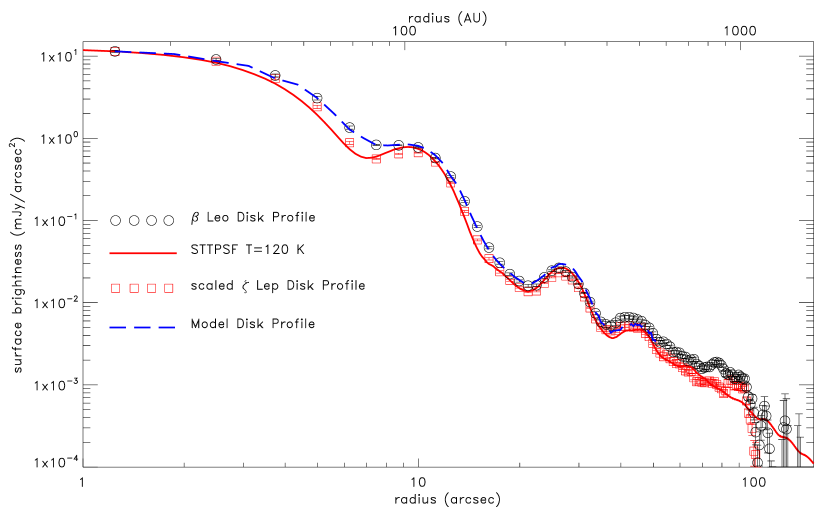
Figure 5.— The azimuthally averaged radial profile of the $\beta$ Leo disk at 24 µm shown in open circles compared to the model profile (blue long-dashed line). For comparison, the profiles made from point sources (STinyTim PSF and unresolved $\zeta$ Lep disk) are shown as the red solid line and open squares, respectively.

The excess flux densities at 24 and 70 µm suggest a color temperature of 119 K. A blackbody emission of 119 K represents the excess emission (from the spectral shape of both the IRS and MIPS-SED data) reasonably well, although the emission at 15–20 µm is a bit low (see Fig. 6). For blackbody-like grains, a dust temperature of $\sim$119 K corresponds to a radial distance of $\sim$20 AU in the stellar radiation field of $\beta$ Leo, consistent with the disk being marginally resolved at 24 µm but not at 70 µm. The total dust luminosity is 1.2$\times$10³⁰ ergs s^-1 based on the 119 K blackbody radiation at the given distance of 11 pc, suggesting a dust fractional luminosity ($f_{d}$) of 2.4$\times$10^-5.

4.2.3 IRS Spectra

As described in Section 2.3, the flux offset between the IRS SL and LL modules due to pointing was corrected using the automatic IRS pipeline. A small residual offset is still evident when comparing the slope of the observed SL spectrum with the slope of the expected photosphere from the Kurucz model. We, therefore, scaled down the extracted SL spectrum by 2.7% so that the join points ($\sim$14.3 µm) between SL and LL modules are smooth. The excess IRS spectrum after photospheric subtraction is shown in Figure 6. At 12 µm, the excess is $\sim$1.3% above the stellar photosphere, but $>$10% for wavelengths longward of 18 µm.

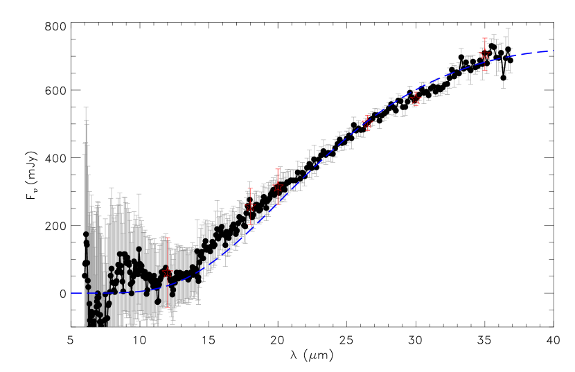
Figure 6.— Spitzer IRS spectrum of the excess emission around $\beta$ Leo (after stellar photospheric subtraction). The error bars include additional 2% errors from the photosphere determination. For comparison, the long-dashed line is the blackbody emission of 119 K normalized to the excesses at 24 and 70 µm. The star-symbols show the 6 fiducial points chosen in our model fitting (see Sec 5.2 for details).

4.3. Interferometric Analysis for $\beta$ Leo

Using the interferometric observations of o Leo, we were able to put constraints on any dust that may be present in the o Leo system and confirm the calibration that was used in the analysis of the $\beta$ Leo system. Details on the interferometric analysis of o Leo are presented in Appendix B.

4.3.1 KIN

The KIN observations of $\beta$ Leo suggest that there is no significant resolved emission at 10 µm in the KIN beam. Limited by its small field of view, our KIN observations are unable to detect extended structures beyond a radius of $\sim$ 3 AU at the distance of $\beta$ Leo (11 pc). Moreover, due to its complex transmission function, KIN observations are most sensitive to extended structures with a radius of less than $\sim$1 AU. From the errors during the April 2008 run, we adopt a 3 $\sigma$ upper limit of 0.9% for the 10 $\mu$m resolved emission, relative to the stellar photosphere. However, due to the complex transmission function of KIN (illustrated in Figure Ab in the appendix), this limit cannot be directly converted into a flux. Instead, we use the Visibility Modeling Tool (VMT) provided by the NASA Exoplanet Science Institute to test different excess configurations and determine how their simulated excesses compare to our limit.

One possible component to any excess detected by KIN is the partially resolved photosphere of $\beta$ Leo itself. If we take the stellar radius to be 1.7 $R_{\sun}$ and assume the star to be uniformly bright, this excess only amounts to 0.2%. While this is well below our detection threshold, it is a constant source of excess that needs to be considered when evaluating models that exceed our 0.9% upper limit.

KIN is most sensitive to emission between $\sim$ 0.05 AU and 1 AU. A disk extending from 0 to 0.05 AU would produce a null above the 0.9% limit only if it were brighter than 645 mJy, whereas a ring between 0.05 and 0.1 AU would be detected if its flux is above 145 mJy at 10 $\mu$m. A uniform disk model extending from 0 to 1 AU will produce an excess greater than 0.9% for 10 µm fluxes above 110 mJy. However, because the sensitivity drops rapidly at AU scales, a similar model extending from 0 to 2 AU will only surpass our 3 $\sigma$ limit if it is at least 240 mJy in brightness. For a 1 to 2 AU ring, the threshold becomes 370 mJy.

The hot excess of $\beta$ Leo detected by Akeson et al. (2009) at 2 $\mu$m is taken to be evidence for a hot inner ring. While there are several models presented in Akeson et al. (2009) that can fit the hot excess, they focus on a ring model extending from 0.13 to 0.43 AU. Such a ring would be above KIN’s 3 $\sigma$ limit if it has a 10 µm excess greater than 96 mJy. Based on their 2 µm excess of 2.7 $\pm$ 1.4 Jy, a normal Rayleigh-Jeans falloff from this point would yield 108 mJy, which is somewhat above our 3 $\sigma$ limit. Thus, the KIN null detection is not consistent with the Akeson et al. (2009) result. There are several possibilities that could explain the discrepancy. It is possible that the excess is more compact than the suggested model. However, to avoid being detected in KIN, the excess would have to be closer to the star than 0.1 AU (if it is located within a narrow ring) or 0.15 AU (if it is part of a continuous disk extending into the star). In either case, much of the disk would be located within the sublimation radius for amorphous grains of 0.12 AU (Akeson et al., 2009), making the possibility of such a compact disk unlikely. More likely, the disagreement between KIN and Akeson et al. (2009) suggests that the source of this hot emission is variable, has a color bluer than a normal star (Rayleigh-Jeans), or the emission level is smaller than the reported value.

4.3.2 BLINC

To compare physical models of the $\beta$ Leo disk to the BLINC data (shown in Figure 2), a program was created to take an input disk geometry, interfere it, convolve it with the aperture PSF and pass it through the same data reduction pipeline used on real images. Because of the limited datapoints, these calculations assumed an optically and geometrically thin disk composed of blackbody grains. The dust in the disk was given an optical depth of the form

$$\tau(r)=Cr^{p},$$ (1)

where $C$ is a brightness scaling constant and $p$ is the power law index. Assuming a sharp inner ($R_{in}$) and outer ($R_{out}$) cutoff beyond which $\tau$ is zero, there were four variables: $R_{in}$, $R_{out}$, $C$ and $p$.

We first compare the possible disk geometries from the interferometry, using the integrated excess from the Spitzer observations as an additional constraint. Figure 7 shows a set of disk geometries compared to the source null of $\beta$ Leo. In this and similar figures it should be noted that the hump located near 0$\farcs$8 does not correspond to a physical excess at that separation from the star; rather, it is a feature relating to the PSF of the aperture. The disk geometries in Figure 7 use different brightness scaling constants, $C$, and all assume a uniform ($p$=0) disk that extends from 0 AU to 10 AU. For a uniform disk, the values of $C$ are equivalent to the optical depth of the disk. Disk geometries with $R_{out}>10$ AU do not differ significantly from these simulations, since the BLINC data are not sensitive outside this radius. These models are thus good approximations of continuous disks that extend into the outer regions imaged by Spitzer. The best fit for such a ’continuous disk’ simulation is given as a dotted line in Figure 7, and corresponds to an optical depth of 2.25$\times 10^{-5}$. This geometry has a reduced $\chi$² of 4.2, making it a relatively poor fit. More importantly, such a disk is required to have a flux density of 0.515 Jy at 10.5 µm (or $\sim$9% excess emission above the stellar photosphere). This is inconsistent with the SED-measured excess shown in Figure 3 and the IRS excess spectrum in Figure 6. We therefore rule out a continuous disk extending from 0 AU to 10 AU or beyond as being the source of the excesses measured by BLINC.

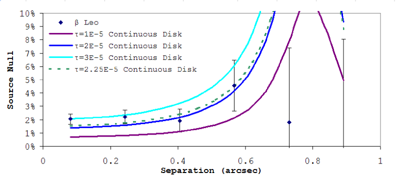
Figure 7.— Continuous disk models for varying brightness constants plotted with $\beta$ Leo strip datapoints as a function of separation from the center. The best fit continuous disk is indicated with a dotted line.

Better fits can be achieved by varying the inner and outer radii. The best possible fits for both a uniform and an inverse ($p=-1$) disk are with a ring extending from 1 to 2 AU. In both models there is a reduced $\chi$² of around 0.7. However, these models require the disk to be even brighter at 10.5 µm than the best fit continuous disk models, and thus are also inconsistent with our other observations. In order to bring the models more in line with the IRS data, we consider only those that are at most 0.30 Jy in brightness ($\sim$5% of the photosphere). Doing so, we find the best fit models to have reduced $\chi$² of around 2. The models are shown in Figure 8. One model assumes a uniform disk and the other assumes an inverse disk. Both of these model disks have an inner radius of 2 AU and a width of less than 1 AU (although the best fit uniform disk is slightly more extended than the best fit inverse disk). Both disks have a flux of 0.30 Jy at 10.5 µm  with the uniform disk having a slightly better reduced $\chi$² ($\chi$² = 1.9) than the inverse disk ($\chi$² = 2.0). The uniform disk has an optical depth of 1.04$\times 10^{-4}$ while the inverse disk has an optical depth of 1.50$\times 10^{-4}$ at $R_{in}$.

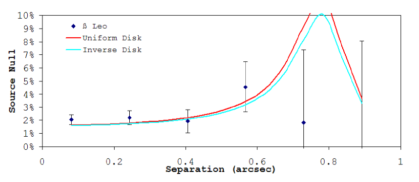
Figure 8.— Best fit models for a uniform disk and an inverse power law disk, given a maximum flux of 0.3 Jy at 10.5 µm. Also plotted are $\beta$ Leo datapoints, as a function of separation from the center.

Overall, both uniform and inverse models are similar with regards to their quality of fit. The similarity of these two cases shows that the best fit is insensitive to the power law index when considering thin rings. Also, as noted above, better fits can be found if we allow for higher fluxes; however, such brighter disks would be inconsistent with other data.

While the above models are the best fits to the BLINC data, $R_{in}$ and $R_{out}$ have some flexibility: $R_{out}$ can be extended to 4 AU before the reduced $\chi$² exceeds 3. Similarly, disks that have brightness less than 0.30 Jy and reduced $\chi$² less than 3 exist for models with $R_{in}$ as small as 1 AU. Reducing $R_{in}$ to less than this extends the disk to regions where BLINC strongly suppresses emission and is thus insensitive, resulting in a rapidly increasing disk brightness while minimally affecting the quality of fit. However, KIN becomes increasingly sensitive to regions inside of $\sim$2 AU, which restricts the amount of excess that can be there and still result in a null detection by KIN. Disk widths larger than 1.5 AU result in poor fits ($\chi$² greater than 3). However, disks narrower than 1 AU do not strongly degrade the fit; at widths less than $\sim$0.5 AU, the resolution of BLINC makes the models degenerate in brightness and width.

With these possible geometries, we look in more detail at the flux constraints from the interferometry. Based on the null analysis in Section 3.1, the excess was found to be 1.74$\pm$0.30% over the photosphere. If we take the photosphere to be 6.3 Jy at 10.5 µm, this excess would be 0.11$\pm$0.02 Jy. However, for a near face-on disk, the interference pattern will suppress at least half of the light, and possibly more depending on the location of the dust, which sets a lower limit of 0.22 $\pm$ 0.04 Jy on the dust emission in this ring. This is consistent with our uniform and inverse model simulations that find that any disk with a flux fainter than 0.2 Jy would result in poor fits. Taking into consideration the IRAC 8 $\mu$m and IRS data, the maximum brightness for this BLINC component is 0.3 Jy.

We have used the VMT to model what level of signal, if any, KIN would see from this belt. We find that a 0.3 Jy belt extending from 2 to 3 AU creates a null in KIN of -0.2%. This negative null is likely due to the complex transmission pattern of KIN (see Figure Ab in the appendix) and the fact that the belt would lie in the sidelobes of this pattern. Combined with the partially resolved photosphere of $\beta$ Leo, the net signal from the system is 0%. For a belt that is less than 0.3 Jy in brightness, the combined null approaches 0.2% (as we would expect). For a belt that has an inner radius as small as 1 AU, the predicted null would still not be large enough to exceed the 0.9% limit that has been established. So, for belts less than 0.3 Jy, the resulting nulls predicted by the VMT are fully consistent with our KIN data. In summary, using the simple models outlined above we then conclude that the excess component detected by BLINC is consistent with a narrow ring of 2–3 AU with a brightness of 0.25$\pm$0.05 Jy at 10.5 $\mu$m.

5. Physical Models of the $\beta$ Leo Debris Disk

We now build a physical model to probe the disk properties (such as the extension and total dust mass) based on all the information derived from interferometric and Spitzer excesses, with assumed grain properties. We start with a simple disk with one component in order to minimize the free parameters being fit to the global excess SED; we then add an additional component required by the spatial constraint provided by the interferometric data.

5.1. Basic SED Model Description

We assume a simple, geometrically-thin (1-D) debris disk where the central star is the only heating source in the system (optically thin). The dust is distributed radially from the inner radius ($R_{in}$) to the outer radius ($R_{out}$), and governed by a power law of radius $r$ for the surface number density with an index $p$ ($\Sigma(r)\sim r^{p}$, $p$ = 0 is a disk with constant surface density expected from a Poynting-Robertson drag dominated disk; while $p$ = –1 is a disk expected from grains ejected out of the system by radiation pressure). We further assume that the grains in the disk have a uniform size distribution at all radii, following a power-law with minimum cutoff radius of $a_{min}$, maximum cutoff radius of $a_{max}$, and a power index of $q$ = –3.5 ($n(a)\sim a^{-3.5}$), consistent with grains generated in theoretical collisional equilibrium. No obvious dust mineralogical features are seen in the IRS spectrum to favor a specific dust composition; therefore, we adopt the grain properties (size-dependent absorption $Q_{abs}$ and scattering $Q_{scat}$) of astronomical silicates (Laor & Draine, 1993) with an assumed grain density of 2.5 g cm^-3. We then compute the dust temperature as a function of the grain size, the incident stellar radiation (best-fit Kurucz model), and the distance $r$ based on balancing the energy between absorption and emission by the dust (scattering is ignored in this simple model). The final SED is then integrated over the grain size and density distribution.

5.2. Main Planetesimal Belt

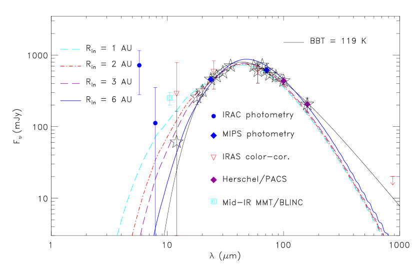
Figure 9.— The excess SED of the $\beta$ Leo disk. Most of the symbols and lines used are defined on the plot, except for the open-star symbols which are the 15 fiducial points used in the $\chi^{2}$ computation.

Figure 9 shows the excess SED of the $\beta$ Leo system. We find that a 119 K blackbody emission matches the excess emission for wavelengths longward of 20 µm. We refer to this excess component as dust from the main planetesimal belt, and try to set constraints using our simple SED model. We first start to fit the SED with $a_{min}\sim a_{bl}$, the smallest grains that are bound to the system against the radiation pressure force, and $a_{max}\sim$1000 µm, the largest grain size in our opacity function. In the case of $\beta$ Leo, $a_{bl}\sim$ 3 µm. Note that grains with sizes larger than 1000 µm contribute insignificantly to the infrared output due to the combination of the grain properties and the steep size distribution. In addition to the MIPS, color-corrected IRAS 60 µm and Herschel PACS broadband photometry, six fiducial points (12, 18, 20, 26.5, 30 and 35 µm as shown in Figure 6) from the IRS spectrum and four points (55.4, 65.6, 75.8 and 86.0 µm) from the MIPS-SED data are selected to compute $\chi^{2}$ in order to determine the best-fit debris disk model (Table 6). We tried both $p$ = 0 and $p$ = –1 cases with various combinations of $R_{in}$ and $R_{out}$. The resultant model emission has a wrong spectral slope in the regions of 15–25 and 55–95 µm. We then tried to relax $a_{min}$ to be larger or smaller than $a_{bl}$ in the fit, and found that the $a_{min}\sim$5 µm with $p$ = 0 case gives the best $\chi^{2}$ value ($\chi_{\nu}^{2}$=0.4). Using the same parameters but with $a_{min}$= 3 µm gives a $\chi_{\nu}^{2}$ value of 2.8. By fixing these parameters ($a_{min}$ = 5 µm, $a_{max}$ = 1000 µm, and $p$ = 0), we can then derive the best-fit inner and outer radii to be 3$\pm$2 AU and 55$\pm$8 AU, respectively, with a total dust mass of (1.9$\pm$0.3)$\times$10^-4 $M_{\earth}$. The SED using these best-fit parameters is shown in Figure 9.

Table 6Excess flux densities used in the SED model

$\lambda$	Flux Density	Error	Source
µm	mJy	mJy
12.00	60.98	102.86	IRS
18.00	256.26	53.73	IRS
20.00	314.69	52.34	IRS
23.68	457.83	40.68	MIPS
26.50	502.92	22.57	IRS
30.00	573.74	20.23	IRS
35.00	705.96	47.58	IRS
55.36	699.79	39.58	MIPS-SED
60.00	598.31	195.11	IRAS
65.56	718.21	66.14	MIPS-SED
71.42	615.25	52.06	MIPS
75.76	531.73	38.21	MIPS-SED
85.96	502.83	75.40	MIPS-SED
100.00	435.58	50.02	PACS
160.00	205.27	46.00	PACS

Based on these parameters from the excess SED, we also construct a model image at 24 µm to compare with the observations. We assume the disk mid-plane is aligned with the stellar equator, inclined by 21.5°. The model image was projected to the inclination angle, and then convolved with model STinyTim PSFs. The azimuthally averaged radial profile computed from the model image is also shown in Figure 5, and matches well with the observed profile at 24 µm. This is consistent with the $\beta$ Leo disk being marginally resolved with a disk radius less than 80 AU.

5.3. Inner Warm Belt

The next step is to see whether the model we construct for the main planetesimal belt is consistent with the resolved structure detected by BLINC. The model excess flux from the main planetesimal belt is $\sim$57 mJy at 10.5 µm, which is lower by a factor of 5 compared to the required level (0.25$\pm$0.05 Jy) to fit the null level derived from the BLINC data. Reducing the inner radius of the main planetesimal belt will increase the flux contribution at 10.5 µm (up to $\sim$130 mJy for $R_{in}=$1 AU); however, it also increases the flux levels in 12–15 µm range, making poor matches with the observed IRS excess (see Figure 9). We also generated high-resolution model images at 10.5 µm given the various inner radii and used them as input to compute the BLINC null levels. The resultant null levels are shown in Figure 11, and they all fail to provide satisfactory fits inside of 0$\farcs$6. Therefore, a surface brightness deficit (gap) in the disk structure is required to explain both the BLINC and Spitzer data.

We then explore the possibility of an inner warm belt separated from the main planetesimal belt. Judging from the amount of excess emission in the range of 5.8–10.5 µm, the typical dust temperature for this emission is $\sim$600 K. From the constraints derived from the BLINC data, we know this warm component is located at 2–3 AU. Figure 10 shows the thermal equilibrium dust temperature distribution around $\beta$ Leo. For astronomical silicate grains with sizes smaller than 1 µm, the thermal equilibrium temperatures are generally lower than 500 K at distances of 2–3 AU from $\beta$ Leo. Only sub-micron-size silicates can reach such a high temperature at a distance of a few AUs. In addition, sub-micron silicate grains have prominent features near 10 and 20 µm. Alternatively, sub-micron carbonaceous grains have equilibrium temperatures of $\sim$600 K, but produce featureless emission spectrum in the infrared.

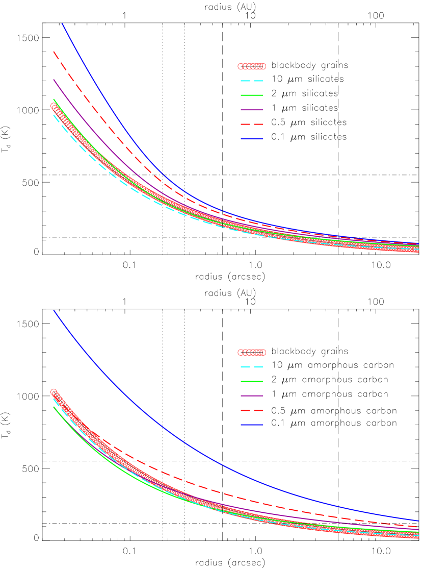
Figure 10.— Thermal equilibrium dust temperature distribution around $\beta$ Leo using grain properties of astronomical silicates (upper panel) and amorphous carbon grains (lower panel).

Due to the uncertainty in the exact amount of excess emission for wavelengths shortward of $\sim$11 µm, we cannot put real constraints on grain compositions and sizes. Our goal is to have the simplest model for the warm belt that can fit the global SED when combined with the emission from the main belt, and with a null level computed from the model image that matches the BLINC data. Given the high dust temperatures in the 2–3 AU belt, we adopted grain properties for amorphous carbon grains (density of 1.85 g cm^-3, Zubko et al. 1996) with a radius of 0.5 µm. The surface density in this warm belt is assumed to be constant (uniform distribution at all radii between 2 and 3 AU). With these assumed parameters, we find that we need very little dust ($M_{d}\sim$2.6$\times$10${}^{-8}M_{\earth}$ or $f_{d}\sim 7.9\times$10^-5) to produce the emission shortward of $\sim$11 µm. Since this warm belt will contribute some fraction of the emission longward of $\sim$11 µm, we have to adjust the inner radius of the main planetesimal belt to 5 AU so the resultant combined excess SED fits the observed IRS spectrum within the errors. The final two-component excess SED is shown in Figure 12, and its corresponding null level is shown in Figure 11 as well. The final parameters for the disk are summarized in Table 7.

Table 7Parameters in the two-component model

Parameters	Inner Warm Disk	Planetesimal Disk
Adopted Grains	Carbonaceous	Silicate
Grain density (g cm-3)	1.85	2.5
Surface density	$\sim r^{0}$	$\sim r^{0}$
$R_{in}$ (AU)	$\sim$2	$\sim$5
$R_{out}$ (AU)	$\sim$3	$\sim$55
$a_{min}$ (µm)	$\sim$0.5	$\sim$5
$a_{max}$ (µm)	$\sim$0.5	1000
$M_{d}$ ($M_{\earth}$)	2.6$\times$10-8	2.2$\times$10-4
$f_{d}=L_{IR}/L_{\ast}$	7.9$\times$10-5	2.6$\times$10-5

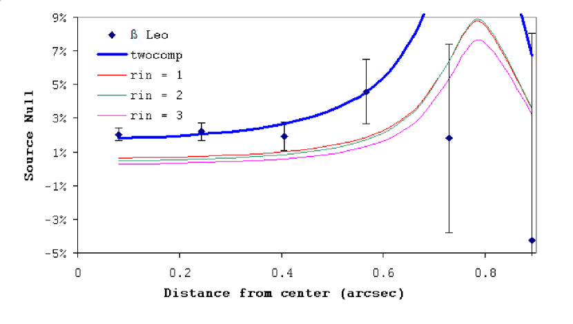
Figure 11.— The computed null levels based on the model images for $\beta$ Leo. Models based on one main planetesimal belt with various inner radii are shown as thin solid lines. Compared to the observed null data points (diamonds), these one-component models do not provide good fits. The computed null level based on the two-component model (main planetesimal belt plus a separate warm belt) is shown as the thick solid line, which provides a better fit to the observed data.

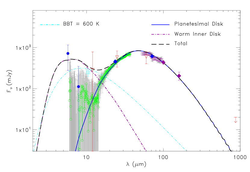
Figure 12.— The SED for the final, two-component disk model. Symbols used are the same as in Figure 9

6. Discussion

From the infrared excesses detected from the ground-based interferometric and Spitzer data, the debris disk around $\beta$ Leo has two distinct dust components: a main planetesimal belt distributed from $\sim$5–55 AU that contains second generation dust grains produced by collisional cascades from large parent bodies residing in this main belt, and a thin warm belt confined mostly to $\sim$2–3 AU. Our simple model (having uniform density distributions in both the inner and outer components) suggests that the debris disk around $\beta$ Leo has a physical gap ($\sim$3–5 AU) separating the two components. Since the gap is not near the ice sublimation regions of $\beta$ Leo ($\sim$10 AU), sublimation is unlikely to be the cause for the absence of a measured excess. Because the resolved excess emission is only detected at a single wavelength (N band), we cannot rule out the possibility that the gap is due to a combination of disk density variations and the resultant temperature structure, which could cause a surface brightness deficit at 10 $\mu$m, rather than a real physical gap. Nevertheless, we believe the gap is most likely due to the presence of an unseen planetary body. This kind of gap is known to exist in Saturn’s ring, created by the embedded moons directly or by the orbital resonances of the moons.

It is instructive to compare the detected emission at 10 µm  to the emission from the zodiacal dust disk. Indeed, this comparison is often used to gauge the level of difficulty in direct imaging of planets, either via a coronagraph, or an infrared interferometer (Beichman et al., 2006). A model of the solar zodiacal dust provided by Kelsall et al. (1998) accurately predicts the emission seen in the DIRBE observations. For this comparison, the dust is assumed to be a continuous distribution, defined by the Kelsall model, with an inner radius due to dust sublimation ($\sim$0.03 AU for the sun, $\sim$0.15 AU for $\beta$ Leo) and an outer radius that is defined so as not to affect the amount of infrared emission (3 AU for the sun, 10 AU for $\beta$ Leo) measured in the nulled output.

For the BLINC observations a null of 1.7$\pm 0.3$% is fit by a Kelsall model which is 380$\pm$70 times as dense as the solar zodiacal dust disk, or 380 zodies. If the disk were similar in distribution to the solar zodiacal disk, we would expect KIN to measure a similar null level (since the disk is well-resolved by both interferometers). However, the KIN 3 sigma upper limit of 0.9%, when compared to the Kelsall model, suggests that $<$ 130 zodies of material is present. The measurements indicate the current level of knowledge we can obtain for zodiacal dust around nearby stars for direct imaging, and highlight the potential danger of using a single ”zody” measurement in characterizing the dust around stars of interest.

The extension of the main dust belt (radius of $\sim$55 AU) around $\beta$ Leo seems to be small compared to other A-type debris disks at similar age ($\sim$100 AU scale such as the narrow rings around HR4796A (Schneider et al., 2009) and Fomalhaut (Kalas et al., 2005), or a few 100 AU scale for the large disks around Vega (Su et al., 2005) and HR8799 (Su et al., 2009)). The dust mass (summed up to 1000 µm) is $\sim$10 times less massive than the debris disks around the A-stars Vega and Fomalhaut, and $\sim$100 times less than the HR 8799 disk, suggesting that the $\beta$ Leo disk was either born with a low-mass disk or has been through major dynamical events that have depleted most of the parent bodies.

Akeson et al. (2009) also reported imaging of $\beta$ Leo using the Mid-Infrared Echelle Spectrometer (MICHELLE; Glasse & Atad-Ettedgui 1993) on the Gemini North telescope, and found the disk is unresolved at 18.5 µm. Based on our model image at 18.5 µm (after being convolved with a proper instrumental PSF), the brightest part of the disk is $\sim$0.55 mJy pixel^-1 at $r\sim$0$\farcs$6 ($\sim$FWHM of a point source) from the star and 0.2 mJy pixel^-1 at $r\sim$1$\farcs$2 ($\sim$2 FWHM of a point source). Given the observational depth ($\sim$0.55 mJy pixel^-1 on background), it is not surprising that the disk is not resolved at 18.5 µm.

Since the longest wavelength that has a sound infrared excess around $\beta$ Leo is at 160 µm, our observations are not sensitive to very cold grains that emit mostly in the sub-millimeter and millimeter wavelengths. Nevertheless, we can set some constraints based on the Herschel 160 µm data and the 870 µm and 1.3 mm upper limits from Holmes et al. (2003). These upper limits suggest that $\lesssim$37 K dust can hide in the system without being detected, which corresponds to a location $>$200 AU for blackbody-like grains. For a simple uniform-density ring from 200–250 AU consisting of silicate grains of 100–1000 µm  a total dust mass less than $\sim$3$\times 10^{-3}M_{\earth}$ (3-$\sigma$) can exist in this outer part of the $\beta$ Leo disk. Such a cold ring, if it exists, would have a clear separation from the main planetesimal belt ($<$80 AU).

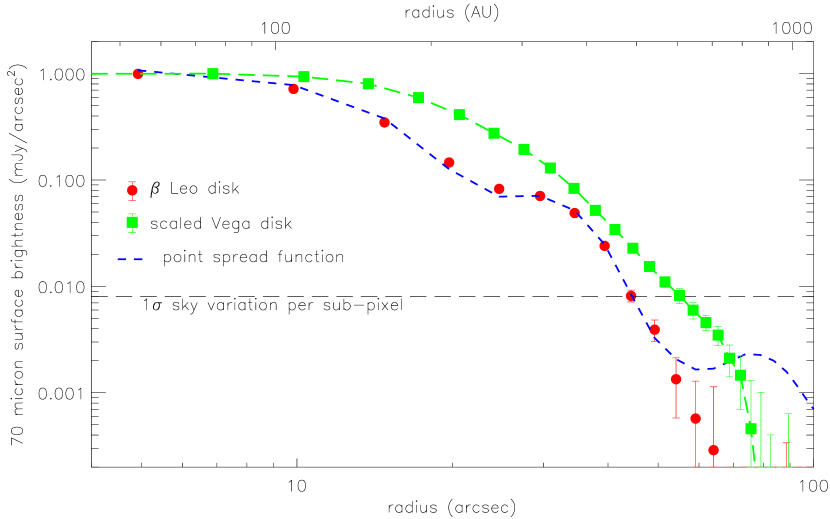
Figure 13.— The azimuthally averaged radial profile of the $\beta$ Leo disk at 70 µm shown in circles compared to the PSF (dashed line). For comparison, we also show the Vega disk profile (squares) that has been scaled to match the same distance and the peak surface brightness as the $\beta$ Leo disk.

There are 12 A-type debris disks, selected from Su et al. (2006), which have ages between 150 and 400 Myr, spectral types between A0 V and A3V, and $f_{d}$ between 10^-5 and 10^-4 (for details see Su et al. 2008). Only the disks around Vega (Su et al., 2005) and $\gamma$ Oph (Su et al., 2008) show large disk extension at 70 µm (radius $\sim$800 AU for Vega and $\sim$520 AU for $\gamma$ Oph), while the rest of them have outer disk radii within 200 AU (Su et al. 2010, in prep.). For a direct comparison, we have rescaled the Vega disk to the same distance as $\beta$ Leo, matched the peak surface brightnesses in the disks at 70 µm, and compared the radial surface brightness profiles (see Fig. 13). If the $\beta$ Leo disk had a halo similar to the Vega disk, we would have detected it at $>$10 $\sigma$ levels (at radii of 200–300 AU) around $\beta$ Leo. This suggests that the mechanism that is responsible for creating such a large halo around Vega does not operate in $\beta$ Leo.

7. Conclusion

Using an array of instruments on Spitzer (imaging, photometry and spectroscopy) as well as 10 µm nulling interferometry on AU and sub-AU scales with the MMT and Keck, we have examined the $\beta$ Leonis system and characterized its debris disk. We have found the system to have at least two distinct components: a warm, narrow ring located near 2 AU and a broad, cooler ring extending from 5 to 55 AU. We also find the system to lack any significant belt beyond 80 AU, which is in contrast to many other A-stars with debris disks. Although not examined in detail here, the truncation of the outer disk may be indicative of disruption at some point in its history or the presence of larger planetary bodies, while the existence of a two-component debris disk may similarly indicate the presence of planets in the inner parts of the system.

Appendix A Nulling Interferometry with BLINC

Nulling interferometry allows light from a central source to be suppressed, while not affecting surrounding, extended emission. Consequently, fainter sources surrounding a central source can be more easily observed.

Nulling interferometry using BLINC on the MMT operates by splitting the incoming light into two subapertures. By requiring light from one subaperture to travel an additional distance of half a wavelength and then recombining the two lightpaths, a transmission pattern is created with the form

$$T(\theta)=\sin{}^{2}(\frac{\pi b\theta}{\lambda})$$ (A1)

where $b$ is the interferometer baseline, $\lambda$ is the wavelength of light and $\theta$ is the vertical angular distance from the central null. Figure Aa shows the transmission pattern created by BLINC for the simplified case of uniform contribution from 8 to 13 µm. Using this pattern, the flux from the central star is strongly suppressed while extended structures, such as debris disks, are much less affected (Hinz et al., 2000). With a baseline of 4m (which is the separation of the subapertures used on the MMT), the first constructive peak occurs at 0$\farcs$25; however, BLINC is sensitive to emission outwards of 0$\farcs$12, where the transmission is neither destructive nor constructive. This system is ideal for probing regions containing warm disks around nearby main sequence stars. Moreover, using the adaptive optics systems on the MMT, we can obtain stable, diffraction limited images. This allows the pathlength between beams to remain fixed instead of varying randomly. Such random variations would require less efficient techniques, such as ’lucky imaging,’ to extract useful data (Hinz et al., 2001).

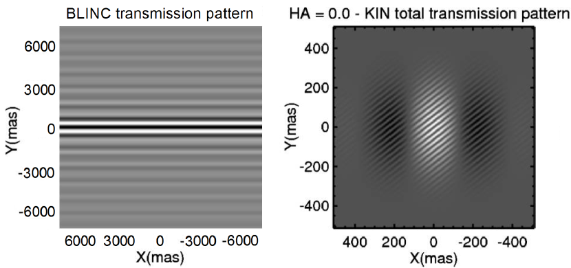
Figure A.— (a) The combined N-band transmission pattern for BLINC on the detector. (b) The 10 µm transmission pattern for KIN, combining the pupil transmission, long baseline fringes and cross-combiner fringes for 0 hour angle and +20 degrees declination. From Colavita et al. (2009).

To set the appropriate pathlength difference between beams that will achieve destructive or constructive interference, prior to each dataset a pair of calibrator frames is taken. A calibrator frame consists of changing the pathlength to an intermediate distance (neither constructive nor destructive). For each calibrator pair, one frame is taken on the shortward side of the optimal pathlength and the other on the longward side. The observed brightness of the star for these calibrator frames is directly proportional to the transmissive efficiency; when BLINC is properly set to destructive interference, the brightness of the star will be the same for both calibrator frames ($I_{1}$ = $I_{2}$). If the pathlength difference is not properly set for destructive interference, the calibrator frames will be different brightnesses. To correct BLINC, the optimal pathlength can be approximated using

$$Correction=g\frac{I_{1}-I_{2}}{I_{1}+I_{2}}$$ (A2)

where $g$ is a constant gain factor which has been set experimentally using an artificial source. While this procedure will set BLINC to optimal destructive interference for moderate offsets, if the initial offset is too large, BLINC may settle into a side null. These nulls are 15-20% worse than the central null while variations from dataset to dataset are much smaller (typically several percent, see Figure 1). Consequently, data taken at the incorrect null are easily identified and removed from the overall dataset.

In order to extract meaningful information, sky subtracted constructive and destructive images of both the science star and a calibrator star need to be obtained. The ”instrumental null” is the null measured by the instrument and is the ratio of a destructive image to a constructive image for a given target. The constructive image allows for the normalization of destructive images to a baseline, in this case the brightness of the central star. For a monochromatic point source perfectly centered in the image, this ratio would be zero, since the target would be perfectly nulled; however, in actual observations, stars will only be incompletely suppressed, typically yielding a ratio of $\sim$ 3% , with some amount of variation from frame to frame. Thus a calibrator star is needed to set a baseline with which to compare a science star (in this case, $\beta$ and o Leo). For such science stars, the ”source null” refers to the instrument null of the science star subtracted by the instrument null of a calibrator star. If the science star is unresolved (i.e. a point source), then the source null will be zero within the error bars. If the star is resolved, then the source null will be positive. By calculating the source null at different size scales, spatial information on the object can be gained.

Appendix B Interferometric Analysis for o Leo

B.1. KIN

We use a simple model, created with the Visibility Modeling Tool (VMT) provided by the NASA Exoplanet Science Institute. The tool allows one to create a hypothetical system, consisting of any number of point sources, disks and rings that may be either uniform or Gaussian, and predicts the observational signature if the hypothetical system were to be observed by KIN. We used the model to test whether the variation in null detected can be explained solely by the stellar components of the binary system. Hummel et al. (2001) determine the necessary stellar parameters and orbital data necessary to model the system with two point sources. We adopt a difference in N-band magnitude between the primary and secondary of $\delta m_{N}=1.5$. Given an orbital period of 14.5 days for the stellar pair, we can use the date of the observations to estimate the relative positions of the primary and secondary to determine a hypothetical observational signature. Values calculated for the expected and observed nulls are shown in Table 8. Comparing the two, we can say that the predicted and actual data are marginally consistent, indicating little evidence for additional extended emission.

Table 8Observed and Expected Nulls for o Leonis

Date	Obs. Null (%)	Expect. Null (%)1
16 Feb 2008	$-0.4\pm 1.0$	$0.87\pm 0.63$
17 Feb 2008	$3.6\pm 0.3$	$1.35\pm 0.98$
14 Apr 2008	$1.7\pm 1.0$	$0.83\pm 0.60$

Note. — 1 - The errors quoted are estimates, incorporating the effects of: 1) the change in interferometer baseline orientation relative to the sky over the time of observation (typically about 1 hour); 2) uncertainty in the calculated relative positions of the stellar components; 3) the error in the N-band flux ratio between the stellar components.

Given the behavior of the null with respect to time as compared to the detailed orbital parameters determined by Hummel et al. (2001), we can conclude that the non-zero nulls detected by our KIN observations are likely due to the stellar components being resolved, with no evidence for excess emission from warm dust. A conservative 3 $\sigma$ upper limit for 10 $\mu$m emission from hot dust in the system can be taken to be 3%.

B.2. BLINC

Although there was no significant excess emission around o Leo, we can set constraints on what dust might be present there. o Leo is a spectroscopic binary located at a distance of 41.5 pc with a separation of 0.21 AU (making the semi-major axis 5 mas). The orbit has a 57.6 degree inclination from face on (Hummel et al., 2001), and we will make the assumption that any circumbinary debris disk will have a similar inclination to us.

If we assume blackbody grains and the above parameters for the system, we can calculate the radius where we would expect to find 300K grains. This is the temperature at which the blackbody emission peaks around 10 µm. The physical parameters for the host stars are derived to be 5.9R_⊙ and 6000 K for the first star and 2.2R_⊙ and 7600 K for the second star (Hummel et al., 2001). For spherical blackbody grains,

$$T_{g}=(\frac{T_{1}^{4}R_{1}^{2}+T_{2}^{4}R_{2}^{2}}{2r^{2}})^{.25}$$ (B1)

So $T_{g}$ = 300 K when $r$ = 9 AU, which for o Leo is at an angular separation of 0$\farcs$22 along the semi-major axis. Assuming the disk is oriented vertically on the detector (and thus perpendicular to the interference pattern), this would put such a ring close to the constructive peak, making BLINC especially sensitive to any dust located in that region.

Figure B shows the source null of several ring models plotted along with the o Leo datapoints. The models assume the orientation of the disk is perpendicular to the interference pattern of the interferometer. The optical depth of each model is listed in the legend, and the rings extend from 8 to 10 AU, directly through the 300 K region around the star. Plotted as a dotted line is the 2 $\sigma$ limit (based on the error bars of each datapoint) above which we would have a marginal detection. Thus, if there were a dust ring equivalent to the 3.75$\times 10^{-4}$ model in Figure B, we would not expect to have a positive detection, whereas we would expect to have gotten a marginal detection if the dust ring had an optical depth of 5$\times 10^{-4}$. Since models that are brighter than $\sim$3.75$\times 10^{-4}$ begin to lie above the 2 $\sigma$ threshold, this model marks the upper limit we can place on dust in such a ring, which corresponds to a flux of 0.17 Jy at 12 µm.

If, on the other hand, the disk were oriented parallel to the interference pattern, a brighter disk could be present without being detected. For this sub-optimal orientation, an upper limit of 0.31 Jy can be placed on the disk.

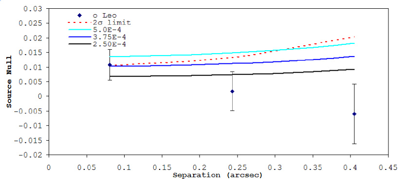
Figure B.— Ring models (8–10 AU) of varying optical depth for o Leo. The semi-major axis is aligned perpendicular to the interference pattern. The dotted line represents the 2 $\sigma$ detection limit based on our observations. Also shown is the source null for o Leo, originally plotted in Figure 2b.

B.3. Comparison to previous measurements

o Leo has previously been identified as having a very hot excess by Trilling et al. (2007) using MIPS on Spitzer. Trilling et al. (2007) reported a 24 and 70 $\mu$m excess ratios for o Leo of 1.23 and 1.30 respectively, suggesting the presence of circumbinary dust. They derived a dust temperature of 815 K with a minimum radius of 0.85 AU (0$\farcs$02). Although too concentrated to be detectable by BLINC, such a disk would be odds with the lack of detection by KIN. However, Trilling et al’s analysis appears to be based on saturated 2MASS measurements for o Leo, from which they derive a K-band magnitude of 2.58 $\pm$ 0.15. If instead we use Johnson K-band photometry (Johnson et al., 1966) converted to a 2MASS K_S magnitude, we find that o Leo is 2.39 $\pm$ $<$0.07, 0.19 magnitudes brighter than calculated by Trilling et al. Since the 2MASS data is saturated for o Leo, we believe this Johnson K-magnitude to be a better measurement. Using this magnitude, our model fitting predicts flux densities of 816 and 89.5 mJy (or ratios of 1.00 and 1.06 to the stellar photosphere) respectively at 24 and 70 µm. The MIPS measurements reported by Trilling et al. (2007) then indicate no excess at 24 $\mu$m above the $\sim$ 6% (2-$\sigma$) level (and above 15% at 70 $\mu$m). The new ratios indicate that the system harbors little, if any, dust. The lack of excess detections at longer wavelengths is then consistent with the null detections by BLINC and KIN at 10 µm.

References

- Absil et al. (2006) Absil, O. et al. 2006, A&A, 452, 237
- Akeson et al. (2009) Akeson, R. L., et al. 2009, ApJ, 691, 1896
- Aumann (1985) Aumann, H. H. 1985, PASP, 97, 885
- Backman & Paresce (1993) Backman & Paresce 1993, Protostars and Planets III, p1253
- Beichman et al. (2006) Beichman, C. A., et al. 2006, ApJ, 652, 1674
- Bouwman et al. (2008) Bouwman, J., et al. 2008, ApJ, 683, 479
- Carpenter et al. (2008) Carpenter, J. M., et al. 2008, ApJS, 179, 423
- Castelli & Kurucz (2003) Castelli, F., & Kurucz, R. L. 2003, IAU Symposium, 210, 20P
- Colavita et al. (2009) Colavita, M. M., et al. 2009, PASP, 121, 1120
- Colavita et al. (2008) Colavita, M. M., et al. 2008, Proc. SPIE, 7013,
- Colavita et al. (2006) Colavita, M. M., Serabyn, G., Wizinowich, P. L., & Akeson, R. L. 2006, Proc. SPIE, 6268,
- Decin et al. (2003) Decin, L., Vandenbussche, B., Waelkens, K., Eriksson, C., Gustafsson, B., Plez, B., & Sauval, 2003, A&A, 400, 695
- Dent et al. (1995) Dent, W. R. F., Greaves, J. S., Mannings, V., Coulson, I. M., & Walther, D. M. 1995, MNRAS, 277, L25
- Di Folco et al. (2004) Di Folco, E., Thévenin, F., Kervella, P., Domiciano de Souza, A., Coudé du Foresto, V., Ségransan, D., & Morel, P. 2004, A&A, 426, 601
- Engelbracht et al. (2007) Engelbracht, C. W., et al. 2007, PASP,119, 994
- Evans et al. (2003) Evans, N. J., II, et al. 2003, PASP, 115, 965
- Fazio et al. (2004) Fazio, G. G., et al. 2004, ApJS, 154, 10
- Glasse & Atad-Ettedgui (1993) Glasse, A. C., & Atad-Ettedgui, E. I. 1993, Proc. SPIE, 1946, 629
- Gordon et al. (2005) Gordon, K. D., et al. 2005, PASP, 117, 503
- Gordon et al. (2007) Gordon, K. D., et al. 2007, PASP, 119, 1019
- Higdon et al. (2004) Higdon, S. J. U., et al. 2004, PASP, 116, 975
- Hinz et al. (2000) Hinz, et al. 2000, Proc. SPIE, 4006, 349
- Hinz et al. (2001) Hinz, et al. 2001, ApJL 561, 131
- Holmes et al. (2003) Holmes, E. K., Butner, H. M., Fajardo-Acosta, S. B., & Rebull, L. M. 2003, AJ, 125, 3334
- Houck et al. (2004) Houck, J. R., et al. 2004, ApJS, 154, 18
- Hummel et al. (2001) Hummel, et al. 2001, ApJ 121, 1623
- Jayawardhana et al. (2001) Jayawardhana, R., Fisher, R. S., Telesco, C. M., Piña, R. K., Barrado y Navascués, D., Hartmann, L. W., & Fazio, G. G. 2001, AJ, 122, 2047
- Johnson et al. (1966) Johnson, H. L., Iriarte, B., Mitchell, R. I., & Wisniewski, W. Z. 2006, Comm. LPL, 4, 99
- Kalas et al. (2005) Kalas, et al. 2005, Nature 435 1067
- Kelsall et al. (1998) Kelsall, et al. 1998, ApJ, 508, 44
- Kervella & Domiciano de Souza (2007) Kervella, P., & Domiciano de Souza, A. 2007, A&A, 474, L49
- Kervella et al. (2008) Kervella, P., Domiciano de Souza, A., & Bendjoya, P. 2008, A&A, 484, L13
- Kervella et al. (2009) Kervella, P., Domiciano de Souza, A., Kanaan, S., Meilland, A., Spang, A., & Stee, P. 2009, A&A, 493, L53
- Koresko et al. (2006) Koresko, C., Colavita, M. M., Serabyn, E., Booth, A., & Garcia, J. 2006, Proc. SPIE, 6268,
- Laor & Draine (1993) Laor, A. & Draine, B. T. 1993, ApJ, 402, 441
- Lowrance et al. (2005) Lowrance, P. J., et al. 2005, AJ, 130, 1845
- Lu et al. (2008) Lu, N., et al. 2008, PASP, 120, 328
- Marengo et al. (2009) Marengo, M. et al. 2009, ApJ, 700, 1647
- Matthews et al. (2010) Matthews, B. C. et al. 2010, A&A, in press.
- Meyer et al. (2006) Meyer, M. R., et al. 2006, PASP, 118, 1690
- Moshir (1989) Moshir, M. 1989, IRAS Faint Source Catalog, , Version 2.0 (Pasadena: IPAC)
- Rieke et al. (2004) Rieke, G. H., et al. 2004, ApJS, 154, 25
- Rieke et al. (2005) Rieke, G. H., et al. 2005, ApJ, 620, 1010
- Schneider et al. (2009) Schneider, G., Weinberger, A. J., Becklin, E. E., Debes, J. H., & Smith, B. A. 2009, AJ, 137, 53
- Schuster et al. (2006) Schuster, M. T., Marengo, M., & Patten, B. M. 2006, Proc. SPIE, 6270
- Sokolov (1995) Sokolov, N. A. 1995, A&AS, 110, 553
- Song et al. (2001) Song, I., Caillault, J.-P., Barrado y Navascués, D., & Stauffer, J. R. 2001, ApJ, 546, 352
- Stansberry et al. (2007) Stansberry, J. A., et al. 2007, PASP, 119, 1038
- Stapelfeldt et al. (2004) Stapelfeldt et al. 2004, ApJL, 154, 458
- Su et al. (2005) Su, K. Y. L., et al. 2005, ApJ, 628, 487
- Su et al. (2006) Su, et al. 2006, ApJ, 653, 675
- Su et al. (2008) Su, et al. 2008 ApJ, 679, L125
- Su et al. (2009) Su, K. Y. L., et al. 2009, ApJ, 705, 314
- Swain et al. (2008) Swain, M. R., et al. 2008, ApJ, 674, 482
- Telesco et al. (2005) Telesco, C. M. et al. 2005, Nature, 433, 133
- Tokunaga (2000) Tokunaga, A. T. 2000, Allen’s Astrophysical Quantities, 143
- Trilling et al. (2007) Trilling, et al. 2007, ApJ 658, 1289
- van Leeuwen (2007) van Leeuwen, F. 2007, A&A, 474, 653
- Weintraub & Stern (1994) Weintraub, D. A., & Stern, S. A. 1994, AJ, 108, 701
- Wyatt (2008) Wyatt, M. C. 2008, ARAA, 46, 339
- Zubko et al. (1996) Zubko, V. G., Mennella, V., Colangeli, L., & Bussoletti, E. 1996, MNRAS, 282, 1321