Resistivity-driven State Changes in Vertically Stratified Accretion Disks

Abstract

We investigate the effect of shear viscosity, $\nu$, and Ohmic resistivity, $\eta$ on the magnetorotational instability (MRI) in vertically stratified accretion disks through a series of local simulations with the Athena code. First, we use a series of unstratified simulations to calibrate physical dissipation as a function of resolution and background field strength; the effect of the magnetic Prandtl number, $P_{\rm m}=\nu/\eta$, on the turbulence is captured by $\sim 32$ grid zones per disk scale height, $H$. In agreement with previous results, our stratified disk calculations are characterized by a subthermal, predominately toroidal magnetic field that produces MRI-driven turbulence for $|z|\lesssim 2H$. Above $|z|\sim 2H$, magnetic pressure dominates and the field is buoyantly unstable. Large scale radial and toroidal fields are also generated near the mid-plane and subsequently rise through the disk. The polarity of this mean field switches on a roughly 10 orbit period in a process that is well-modeled by an $\alpha$–$\Omega$ dynamo. Turbulent stress increases with $P_{\rm m}$ but with a shallower dependence compared to unstratified simulations. For sufficiently large resistivity, $\eta\sim c_{\rm s}H/1000$ where $c_{\rm s}$ is the sound speed, MRI turbulence within $2H$ of the mid-plane undergoes periods of resistive decay followed by regrowth. This regrowth is caused by amplification of toroidal field via the dynamo. This process results in large amplitude variability in the stress on 10 to 100 orbital timescales, which may have relevance for partially ionized disks that are observed to have high and low accretion states.

¹ jbsimon@jila.colorado.edu, JILA, University of Colorado, 440 UCB, Boulder, CO 80309-0440
Department of Astronomy, University of Virginia, P.O. Box 400325, Charlottesville, VA 22904-4325
² jh8h@virginia.edu, Department of Astronomy, University of Virginia, P.O. Box 400325
Charlottesville, VA 22904-4325
³ kris.beckwith@jila.colorado.edu, JILA, University of Colorado, 440 UCB, Boulder, CO 80309-0440

1 Introduction

Disk accretion is a fundamental astrophysical process, responsible for such diverse phenomena as the immensely luminous, distant quasars and the formation and evolution of protostellar systems. This process requires removing angular momentum from the orbiting gas, and from the beginnings of disk theory it has been clear that microphysical viscosity is orders of magnitude too small to account for observed accretion rates. It is now understood that accretion is driven by magnetohydrodynamic (MHD) turbulent stresses arising from a robust and powerful instability known as the magnetorotational instability (MRI) Balbus & Hawley (1991, 1998).

Analytic investigations of the MRI have proven to be very insightful (e.g., Balbus & Hawley, 1991; Goodman & Xu, 1994), but they can offer only limited guidance to the behavior of the MRI in the fully turbulent saturated state. Numerical simulations have become the essential tool for investigating how the MRI operates in accretion disks, and in particular, local shearing box simulations (see Hawley et al., 1995) have proven to be especially useful in such studies. The shearing box system solves the equations of MHD in a local, co-rotating patch of an accretion disk. The size of this patch is assumed to be small compared to its radial distance from the central star, allowing one to use Cartesian geometry while retaining the essential dynamics of differential rotation. Shearing box simulations have led to an improved understanding of MRI turbulence while addressing some basic questions about accretion disks.

One such question is, what sets the saturation level of MRI-driven turbulence and the angular momentum transport rate? This is usually phrased as “What is $\alpha$?” following Shakura & Syunyaev (1973) who made the ansatz that the $r\phi$ component of the turbulent stress, $\tau_{r\phi}$, is proportional to the pressure, $\tau_{r\phi}=\alpha P$. Previous shearing box simulations have found substantial evidence that MRI-driven stress does not behave in a manner consistent with how $\alpha$ is often applied in disk theory. The early studies of Hawley et al. (1995) showed that the stress is proportional to the magnetic pressure, but the magnetic pressure is not itself directly determined by the gas pressure, a result that holds over a wide range of shearing box simulations (Blackman et al., 2008). Sano et al. (2004) performed an extensive survey and observed, at best, only a very weak gas pressure dependence for turbulent stress. More recently, vertically stratified local simulations of radiation-dominated disks Hirose et al. (2009) have shown that while there is a correlation between the MRI stress and total (gas plus radiation) pressure, it has the opposite causal relationship from that normally assumed in the $\alpha$ model: the stress determines the pressure, not the other way around. Increased stress can lead to increased pressure through turbulent heating, but an increase in pressure does not feed back into the stress.

What then does determine the saturation level of the MRI? We know that viscosity and resistivity can significantly affect the properties of the linear MRI by reducing growth rates and altering the stability limits. Recently, the influence of the viscous and Ohmic dissipation on MRI-induced turbulence has become a focus of shearing box simulations. Previous investigations into the effect of Ohmic resistivity on the saturated state Hawley et al. (1996); Sano et al. (1998); Fleming et al. (2000); Sano & Inutsuka (2001); Ziegler & Rüdiger (2001); Sano & Stone (2002b) found that angular momentum transport decreases as the resistivity is increased, but it was not until the very recent work of Fromang & Papaloizou (2007), Pessah et al. (2007), and Fromang et al. (2007) that the influence of physical dissipation in numerical simulations was fully appreciated. Fromang & Papaloizou (2007) and Pessah et al. (2007) found that for shearing box simulations without a net magnetic flux and without explicit dissipation terms, the turbulent saturation level decreases with increasing numerical resolution without any sign of convergence. This surprising result was subsequently confirmed with different numerical codes (e.g., Simon et al., 2009; Guan et al., 2009). In a second paper, Fromang et al. (2007) demonstrated that the saturation level of the MRI in shearing boxes depends strongly on the magnetic Prandtl number, i.e., the ratio of viscosity to resistivity ($P_{\rm m}=\nu/\eta$). Specifically, for local simulations without a net magnetic flux, the turbulent stresses increase nearly linearly with $P_{\rm m}$ and for $P_{\rm m}\lesssim 1$, the turbulence decays. Fromang (2010) subsequently showed that at a fixed $P_{\rm m}$, the presence of even a small viscosity and resistivity is sufficient to provide convergence in the zero-net field case. The increase in stress with $P_{\rm m}$ is also present for net vertical fields Lesur & Longaretti (2007) and net toroidal fields Simon & Hawley (2009); for these field geometries, the $P_{\rm m}$ dependence is weaker and turbulence is maintained even for $P_{\rm m}<1$. For the net toroidal field model, only a sufficiently high resistivity could actually kill the turbulence completely Simon & Hawley (2009).

Most of these viscosity and resistivity studies used the unstratified shearing box model where vertical gravity is ignored and periodic boundary conditions are assumed for the vertical direction. Shearing box models that include vertical stratification are more realistic however, and interesting new effects arise when vertical gravity is included. For example, in most such simulations, net toroidal field is generated near the mid-plane via MRI turbulence, buoyantly rises upwards, and is replaced with a field of the opposite sign in the mid-plane region. This behavior happens on a timescale of $\sim 10$ orbits and appears to be indicative of an MHD dynamo operating within the disk (e.g., Brandenburg et al., 1995; Stone et al., 1996; Hirose et al., 2006; Guan & Gammie, 2010; Shi et al., 2010; Gressel, 2010; Davis et al., 2010). Furthermore, the vertical structure of the disk consists of MRI-turbulent gas that is marginally stable to buoyancy within $|z|\sim 2H$, whereas outside of this region, the gas is magnetically dominated, significantly less turbulent, and buoyantly unstable (e.g., Guan & Gammie, 2010; Shi et al., 2010).

The effects of resistivity on the MRI in vertically stratified shearing boxes has been studied (e.g., Miller & Stone, 2000), but many of these calculations are designed with protostellar systems in mind and employ a very large resistivity to completely quench the MRI and create a “dead zone” near the midplane (e.g., Gammie, 1996; Fleming & Stone, 2003; Fromang & Papaloizou, 2006; Oishi et al., 2007; Turner & Sano, 2008; Ilgner & Nelson, 2008; Oishi & Low, 2009; Turner et al., 2010). The effects of smaller resistivities and of $\nu$ and $P_{\rm m}$ on vertically stratified turbulence has barely been examined. Recently, however, Davis et al. (2010) investigated how the results of Fromang & Papaloizou (2007) and Fromang et al. (2007) might change in the presence of vertical stratification. Davis et al. (2010) considered the zero-net magnetic flux case and employed vertically periodic boundary conditions to ensure that zero net flux was maintained throughout the simulation. They found that without physical dissipation, the volume-averaged stress level reaches a constant value as numerical resolution is increased, in contrast to unstratified simulations where the stress declines. They further examined three $\nu$ and $\eta$ values that lead to a decay of turbulence in unstratified boxes. With vertical gravity, however, these $\nu$ and $\eta$ values lead to large, long timescale fluctuations in the volume averaged stress level; the turbulence saturates at a relatively high level for $\sim$ 100 orbits, then decreases to a lower saturation level for another $\sim$ 100 orbits, and then increases again.

The primary goal of this work is to extend these first results and investigate in more detail how $\nu$ and $\eta$ affect MRI turbulence in vertically stratified shearing boxes. In particular, we consider the origin of the long-term fluctuations seen in Davis et al. (2010), and whether that effect might be relevant to real accretion disks. Since stratification can alter the saturation levels of MRI-induced turbulence, we also investigate whether increasing $P_{\rm m}$ still leads to increased stress levels and how $P_{\rm m}$ affects the dynamo process previously observed in stratified simulations. Finally, these simulations will also serve as an essential starting point for future studies that include more realistic physics, such as temperature- and density-dependent $\nu$ and $\eta$.

The structure of this paper is as follows. In § 2, we describe our evolution equations, parameters, and initial conditions. In § 3, we present a series of unstratified shearing box simulations to calibrate the effects of physical dissipation and serve as controls for the vertically stratified shearing boxes with constant $\nu$ and $\eta$. We discuss our vertically stratified simulations in § 4, which are the primary focus of this paper. The first set of these simulations contain no physical dissipation, and we carry out several analyses to improve our understanding of vertically stratified MRI turbulence. The second set of simulations then includes physical dissipation to study the $P_{\rm m}$ effect. We wrap up with a discussion and our general conclusions in § 5. We also present a detailed description of our numerical algorithm in an Appendix.

2 Method

In this study, we use Athena, a second-order accurate Godunov flux-conservative code for solving the equations of MHD. Athena uses the dimensionally unsplit corner transport upwind (CTU) method of Colella (1990) coupled with the third-order in space piecewise parabolic method (PPM) of Colella & Woodward (1984) and a constrained transport (CT; Evans & Hawley, 1988) algorithm for preserving the ${\bf\nabla}\cdot{\mbox{\boldmath{$B$}}}$ = 0 constraint. We use the HLLD Riemann solver to calculate the numerical fluxes Miyoshi & Kusano (2005); Mignone (2007). A detailed description of the Athena algorithm and the results of various test problems are given in Gardiner & Stone (2005), Gardiner & Stone (2008), and Stone et al. (2008).

Our simulations utilize the shearing box approximation, a model for a local co-rotating disk patch whose size is small compared to the radial distance from the central object, $R_{o}$. We construct a local Cartesian frame, $x=(R-R_{o})$, $y=R_{o}\phi$, and $z$, co-rotating with an angular velocity $\Omega$ corresponding to the orbital frequency at $R_{o}$, the center of the box. In this frame, the equations of motion become (Hawley et al., 1995):

$$\frac{\partial\rho}{\partial t}+{\bf\nabla}\cdot(\rho{\mbox{\boldmath{$v$}}})=0,$$ (1)

$$\frac{\partial\rho{\mbox{\boldmath{$v$}}}}{\partial t}+{\bf\nabla}\cdot\left(\rho{\mbox{\boldmath{$v$}}}{\mbox{\boldmath{$v$}}}-{\mbox{\boldmath{$B$}}}{\mbox{\boldmath{$B$}}}\right)+{\bf\nabla}\left(P+\frac{1}{2}B^{2}\right)=2q\rho\Omega^{2}{\mbox{\boldmath{$x$}}}-\rho\Omega^{2}{\mbox{\boldmath{$z$}}}-2{\mbox{\boldmath{$\Omega$}}}\times\rho{\mbox{\boldmath{$v$}}}+{\bf\nabla}\cdot{\mbox{\boldmath{$T$}}},$$ (2)

$$\frac{\partial{\mbox{\boldmath{$B$}}}}{\partial t}-{\bf\nabla}\times\left({\mbox{\boldmath{$v$}}}\times{\mbox{\boldmath{$B$}}}\right)=-{\bf\nabla}\times\left(\eta{\bf\nabla}\times{\mbox{\boldmath{$B$}}}\right).$$ (3)

where $\rho$ is the mass density, $\rho{\mbox{\boldmath{$v$}}}$ is the momentum density, $B$ is the magnetic field, $P$ is the gas pressure, and $q$ is the shear parameter, defined as $q=-d$ln$\Omega/d$ln$R$. We use $q=3/2$, appropriate for a Keplerian disk. We assume an isothermal equation of state $P=\rho c_{\rm s}^{2}$, where $c_{\rm s}$ is the isothermal sound speed. From left to right, the source terms in equation (2) correspond to radial tidal forces (gravity and centrifugal), vertical gravity, the Coriolis force, and the divergence of the viscous stress tensor, $T$, defined as

$$T_{ij}=\rho\nu\left(\frac{\partial v_{i}}{\partial x_{j}}+\frac{\partial v_{j}}{\partial x_{i}}-\frac{2}{3}\delta_{ij}{\bf\nabla}\cdot{\mbox{\boldmath{$v$}}}\right),$$ (4)

where the indices refer to the spatial components Landau & Lifshitz (1959), and $\nu$ is the shear viscosity. We neglect bulk viscosity. The source term in equation (3) is the effect of Ohmic resistivity, $\eta$, on the magnetic field evolution. Note that our system of units has the magnetic permeability $\mu=1$. Details about the numerical integration of these equations are presented in the Appendix.

For unstratified shearing box simulations, the boundary conditions are periodic for $y$ and $z$, and shearing-periodic for $x$. In stratified simulations, the periodic $z$ boundary conditions are replaced with outflow boundary conditions. The specifics are described in the Appendix.

2.1 Dissipation Parameters

In all of our simulations, $\nu$ and $\eta$ are parameterized in terms of Reynolds numbers. At a scale height, $H$, away from the radial center of the shearing box, the fluid velocity is $|v_{y}|\sim qH\Omega\sim c_{\rm s}$. Thus, the sound speed is a representative velocity for the fluid, and we define the Reynolds numbers as

$$Re\equiv\frac{c_{\rm s}H}{\nu}.$$ (5)

Similarly we define the magnetic Reynolds number,

$$Rm\equiv\frac{c_{\rm s}H}{\eta},$$ (6)

and their ratio, the magnetic Prandtl number,

$$P_{\rm m}\equiv\frac{\nu}{\eta}=\frac{Rm}{Re}.$$ (7)

Because resistivity affects the MRI directly, another useful dimensionless quantity is the Elsasser number

$$\Lambda\equiv\frac{v_{\rm A}^{2}}{\eta\Omega}.$$ (8)

$\Lambda$ can be computed on a zone-by-zone basis, but it is also helpful to calculate an average $\Lambda$ for a simulation. Thus, we can write the characteristic ${\rm Alfv\acute{e}n}$ speed in direction $i$ via the averaged magnetic field in that direction,

$$v_{{\rm A}i}=\sqrt{\frac{\langle B_{i}^{2}\rangle}{\langle\rho\rangle}},$$ (9)

where the angled brackets denote a volume average, and the subscript $i=(x,y,z)$ depending on the direction of interest. In the above definition of $\Lambda$, all three components are used in calculating the ${\rm Alfv\acute{e}n}$ speed. As the Elsasser number approaches unity, resistivity becomes more dominant, stabilizing the MRI. Simon & Hawley (2009) found that turbulence decayed in net toroidal field, unstratified shearing boxes when the Elsasser number was $\lesssim 100$.

Although we focus on physical dissipation, there is numerical dissipation as well. One way to characterize the effects of finite resolution is to compare the characteristic MRI wavelength, $\lambda_{\rm MRI}=2\pi v_{\rm A}/\Omega$ to the grid zone size. Noble et al. (2010) defined this “quality factor” $Q$ as

$$Q_{i}\equiv\frac{\lambda_{{\rm MRI},i}}{\Delta x_{i}}=\frac{2\pi v_{{\rm A}i}}{\Omega\Delta x_{i}}$$ (10)

Again, $v_{{\rm A}i}$ is defined via equation (9). For $Q_{i}\lesssim 6$, the growth of the MRI can be reduced Sano et al. (2004) and the MRI is under-resolved, although this number has some uncertainty and should be taken only as an estimate.

One can also calculate a volume-averaged ${\rm Alfv\acute{e}n}$ speed rather than an ${\rm Alfv\acute{e}n}$ speed determined by the averaged field, i.e.,

$$v_{{\rm A}i}=\left\langle\frac{|B_{i}|}{\sqrt{\rho}}\right\rangle.$$ (11)

For convenience, most of our analysis uses equation (9), as the volume-averaged history data and the one-dimensional, horizontally averaged quantities are routinely computed at high time resolution for use in creating, e.g., space-time plots. As a check, we have calculated the volume-averaged ${\rm Alfv\acute{e}n}$ speed via equation (11) for several hundreds of orbits in a few of our vertically stratified simulations (the volume average is done within $2H$ of the mid-plane). We found that $v_{\rm A}$ from equation (11) is roughly 1-1.5 times larger than that from equation (9).

2.2 Parameters and Initial Conditions

We have run shearing box simulations with different field geometries, dissipation values and resolutions, both with and without vertical gravity. Here, we describe the parameters and initial conditions used in these two types of simulations. The results from the unstratified simulations are presented in § 3 and the results from the stratified simulations are in § 4.

2.2.1 Sine Z Unstratified Simulations

The first set of simulations are unstratified, zero net magnetic flux shearing boxes. This is the same type of problem as investigated in Fromang et al. (2007) and Simon & Hawley (2009). The initial magnetic field is

$${\mbox{\boldmath{$B$}}}=\sqrt{2P_{o}/\beta}~{}{\rm sin}(2\pi x/L_{x})~{}\hat{\mbox{\boldmath{$z$}}}$$ (12)

with $\beta=400$. The isothermal sound speed is $c_{\rm s}=0.001$, corresponding to an initial gas pressure $P_{o}=10^{-6}$ with initial density $\rho_{o}=1$. The orbital velocity of the local domain is $\Omega=0.001$. For these simulations, we define the scale height to be

$$H\equiv\frac{c_{\rm s}}{\Omega}=1,$$ (13)

which is a slightly different definition than that in the stratified box (by a factor of $\sqrt{2}$). The size of the box is $L_{x}=1H$, $L_{y}=4H$, and $L_{z}=1H$. We run several resolutions in order to study convergence, and at each resolution, we study four different cases of $Rm$ and $P_{\rm m}$ values. See Table 1 for the parameters of these runs. The labeling scheme of the runs refers to resolution, field geometry, and dissipation values; e.g.,16SZRm12800Pm16 corresponds to 16 zones per $H$, “SZ” for the “Sine Z” geometry, and $Rm=12800$, $P_{\rm m}=16$. Since, as we will see, $Rm$ is the critical parameter in many of our simulations, we choose to include it as part of the run label, differing from the convention of related works (e.g., Fromang et al., 2007; Simon & Hawley, 2009).

The MRI is seeded with random perturbations to the density and the velocity components introduced at the grid scale. The amplitude of the density perturbations is $\delta\rho=0.01$ and the amplitude of the velocity perturbations is $(1/5)\delta\rho c_{\rm s}$ for each component (a different perturbation is applied for each component). We do not employ orbital advection in these simulations (see Appendix). All simulations are run to 400 orbits, except for the runs in which the turbulence decays and also 32SZRm12800Pm16 and 32SZRe12500Pm4, which were run to 289 orbits and 246 orbits, respectively. We also include the results from previous, higher resolution simulations (Simon & Hawley, 2009) in our analysis.

2.2.2 Flux Tube Unstratified Simulations

The second set of unstratified simulations contain a net toroidal field and are initialized with the twisted azimuthal flux tube of Hirose et al. (2006), with minor modifications to the dimensions and $\beta$ values. The initial conditions are designed to match those used in the vertically stratified simulations of § 2.2.3, so we define $H$ to be that of a stratified, isothermal disk,

$$H=\frac{\sqrt{2}c_{\rm s}}{\Omega}.$$ (14)

The isothermal sound speed, $c_{\rm s}=7.07\times 10^{-4}$, corresponding to an initial value for the gas pressure of $P_{o}=5\times 10^{-7}$. With $\Omega=0.001$, the value for the scale height is $H=1$. As in the SZ simulations, random perturbations are added to the density and velocity components.

The initial toroidal field, $B_{y}$, is given by

$$B_{y}=\left\{\begin{array}[]{ll}\sqrt{\frac{2P_{o}}{\beta_{y}}-\left(B_{x}^{2}+B_{z}^{2}\right)}&\quad\mbox{if $B_{x}^{2}+B_{z}^{2}\neq 0$}\\ 0&\quad\mbox{if $B_{x}^{2}+B_{z}^{2}=0$}\end{array}\right.$$ (15)

and we have run simulations with a toroidal field $\beta$ of $\beta_{y}=$ 100, 1000, and 10000. The poloidal field components, $B_{x}$ and $B_{z}$, are calculated from the $y$ component of the vector potential,

$$A_{y}=\left\{\begin{array}[]{ll}-\sqrt{\frac{2P_{o}}{\beta_{p}}}\frac{H}{2\pi}\left[1+{\rm cos}\left(\frac{2\pi r}{H}\right)\right]&\quad\mbox{if $r<\frac{H}{2}$}\\ 0&\quad\mbox{if $r\geq\frac{H}{2}$}\end{array}\right.$$ (16)

where $r=\sqrt{x^{2}+z^{2}}$ and $\beta_{p}=1600$ is the poloidal field $\beta$ value.

The labeling convention is the same as in § 2.2.1, but with “FT” for “Flux Tube” (see Table 1). We run simulations both with and without physical dissipation. Those simulations with no physical dissipation are labeled with “Num” for “Numerical dissipation”, and for the $\beta_{y}=1000$ (10000) cases, we append $\beta 1000$ ($\beta 10000$) on the end of the run label. The domain size is $L_{x}=2H$, $L_{y}=4H$, and $L_{z}=1H$, and the resolution is 32 zones per $H$. Orbital advection is employed in these calculations (see Appendix). 32FTNum was run to 150 orbits, and both 32FTNum$\beta 1000$ and 32FTNum$\beta 10000$ were run to 110 orbits.

The runs with physical dissipation are initiated from the turbulent state (at $t=100$ orbits) of the corresponding $\beta_{y}$ value run with only numerical dissipation. These simulations were all run out to 220 orbits.

Table 1: Unstratified Simulations

Label	$Re$	$Rm$	$P_{\rm m}$	Resolution	$\alpha$	Description
				(zones per $H$)
16SZRm12800Pm16	800	12800	16	16	0.011	zero net flux
32SZRm12800Pm16	800	12800	16	32	0.033	zero net flux
64SZRm12800Pm16	800	12800	16	64	0.042	zero net flux
128SZRm12800Pm16	800	12800	16	128	0.046	zero net flux
16SZRm12500Pm4	3125	12500	4	16	0.0043	zero net flux
32SZRm12500Pm4	3125	12500	4	32	0.013	zero net flux
64SZRm12500Pm4	3125	12500	4	64	0.015	zero net flux
128SZRm12500Pm4	3125	12500	4	128	0.013	zero net flux
16SZRm6250Pm1	6250	6250	1	16	decay	zero net flux
32SZRm6250Pm1	6250	6250	1	32	decay	zero net flux
64SZRm6250Pm1	6250	6250	1	64	decay	zero net flux
16SZRm25600Pm2	12800	25600	2	16	0.0077	zero net flux
32SZRm25600Pm2	12800	25600	2	32	0.010	zero net flux
64SZRm25600Pm2	12800	25600	2	64	0.0078	zero net flux
32FTNum	–	–	–	32	0.021	flux tube, num. dissipation, $\beta=100$
32FTNum$\beta$1000	–	–	–	32	0.020	flux tube, num. dissipation, $\beta=1000$
32FTNum$\beta$10000	–	–	–	32	0.018	flux tube, num. dissipation, $\beta=10000$
32FTRm800Pm0.5	1600	800	0.5	32	decay	restarted from 32FTNum
32FTRm3200Pm0.5	6400	3200	0.5	32	0.0094	restarted from 32FTNum
32FTRm3200Pm2	1600	3200	2	32	0.018	restarted from 32FTNum
32FTRm3200Pm4	800	3200	4	32	0.028	restarted from 32FTNum
32FTRm6400Pm4	1600	6400	4	32	0.029	restarted from 32FTNum
32FTRm6400Pm8	800	6400	8	32	0.041	restarted from 32FTNum
32FTRm1600Pm1$\beta$1000	1600	1600	1	32	decay	restarted from 32FTNum$\beta$1000
32FTRm3200Pm2$\beta$1000	1600	3200	2	32	0.015	restarted from 32FTNum$\beta$1000
32FTRm3200Pm2$\beta$10000	1600	3200	2	32	decay	restarted from 32FTNum$\beta$10000

2.2.3 Vertically Stratified Simulations

In vertically stratified shearing boxes, the initial density corresponds to an isothermal hydrostatic equilibrium

$$\rho(x,y,z)=\rho_{o}{\rm exp}\left(-\frac{z^{2}}{H^{2}}\right),$$ (17)

where $\rho_{o}=1$ is the mid-plane density, and $H$ is the scale height in the disk, as defined in § 2.2.2. A density floor of $10^{-4}$ is applied to the physical domain as too small a density leads to a large ${\rm Alfv\acute{e}n}$ speed and a very small timestep. Furthermore, numerical errors in energy make it difficult to evolve regions of very small plasma $\beta$. All other parameters and initial conditions are identical to the corresponding FT runs of § 2.2.2. All the stratified runs use $\beta_{y}=100$ for the initial toroidal field strength.

The domain size for all vertically stratified simulations is $L_{x}=2H$, $L_{y}=4H$, and $L_{z}=8H$, and we have run most simulations at 32 grid zones per $H$, with a few at 64 zones per $H$. Orbital advection is employed in all of these runs (see Appendix). The runs are listed in Table 2. The labeling scheme is the same as for the unstratified simulations, but we omit the “FT” label as all the stratified runs use the flux tube initial conditions. We study the effect of physical dissipation by restarting the equivalent resolution, numerical-dissipation-only run at $t=100$ orbits.

Table 2: Vertically Stratified Simulations

Label	$Re$	$Rm$	$P_{\rm m}$	Resolution	Integration time	Description
				(zones per $H$)	$t_{\rm stop}-t_{\rm start}$ (orbits)
32Num	–	–	–	32	1058	num. dissipation
32Rm800Pm0.5	1600	800	0.5	32	263	–
32Rm3200Pm0.5	6400	3200	0.5	32	863	–
32Rm3200Pm2	1600	3200	2	32	1082	–
32Rm3200Pm4	800	3200	4	32	487	–
32Rm6250Pm1	6250	6250	1	32	337	–
32Rm6400Pm8	800	6400	8	32	325	–
32Rm6400Pm4	1600	6400	4	32	488	–
32Rm3200Pm2_By+	1600	3200	2	32	584	$B_{y}$ added at 150 orbits
32ShearBx	–	–	–	32	45	net $B_{x}$ within midplane
64Num	–	–	–	64	159	num. dissipation
64Rm800Pm0.5	1600	800	0.5	64	108	–
64Rm3200Pm0.5	6400	3200	0.5	64	83	–
64Rm3200Pm2	1600	3200	2	64	80	–
64Rm3200Pm4	800	3200	4	64	84	–
64Rm6400Pm4	1600	6400	4	64	80	–

3 Calibration of Physical Dissipation in Unstratified Disks

While our focus is on the effects of physical dissipation on MRI-driven turbulence in stratified disks, we have carried out a series of unstratified shearing box simulations to address several points. First, what resolution is needed to capture the influence of physical dissipation, and how does a given resolution influence the effects due to dissipation terms? Second, what is the effect of physical dissipation on different initial background toroidal field strengths? As we will see, this last question has direct relevance to our stratified simulations, in which the net toroidal field within a given region changes in time via shear and buoyancy.

Table 1 is a list of the unstratified shearing box simulations. The column labeled “Resolution” lists $N_{x}$, the number of zones in one $H$. The column labeled $\alpha$ gives the averaged stress normalized by the averaged gas pressure,

$$\alpha\equiv\frac{\langle\langle\rho v_{x}\delta v_{y}-B_{x}B_{y}\rangle\rangle}{\langle\langle P\rangle\rangle},$$ (18)

where the double brackets denote a time and volume average, the volume average is calculated over the entire simulation domain, and the time average is calculated from orbit 20 to the end of the run. Since the gas is isothermal, $\langle P\rangle=\langle\rho\rangle c_{\rm s}^{2}$.

3.1 Resolving Physical Dissipation

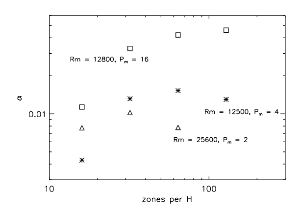
Figure 1: Time- and volume-averaged stress parameter $\alpha$ as a function of grid zones per $H$ in the unstratified SZ simulations; $\alpha\equiv\langle\langle\rho v_{x}\delta v_{y}-B_{x}B_{y}\rangle\rangle/\langle\langle P\rangle\rangle$, where the average is calculated over the entire simulation domain and from 20 orbits to the end of the simulation. Only simulations with sustained turbulence are plotted. The squares are runs with $Rm=12800$, $P_{\rm m}=16$; asterisks are $Rm=12500$, $P_{\rm m}=4$; and triangles are $Rm=25600$, $P_{\rm m}=2$. By 32 zones per $H$, the $\alpha$ values appear to be relatively close to the higher resolution values.

We begin with a resolution study of unstratified simulations with physical dissipation. Figure 1 shows $\alpha$ as a function of resolution for three different $P_{\rm m}$ values in the SZ simulations. The $N_{x}=128$ data listed in the table and plotted in the figure were taken from Simon & Hawley (2009). Note that those runs were similar to, but not the same as those done for this paper. Here, the grid zone size is equal in all directions, $\Delta x=\Delta y=\Delta z$, whereas the Simon & Hawley (2009) runs had $\Delta x=\Delta z=0.4\Delta y$. Furthermore, the calculations done in Simon & Hawley (2009) were performed with the Roe method for the Riemann solver, in contrast to the HLLD solver used here.

For the SZ simulations that have sustained turbulence, $\alpha$ appears to be converging with resolution. More specifically, by 32 grid zones per $H$, $\alpha$ is within a factor of $\sim 1.4$ of the corresponding value at 128 zones per $H$. In contrast, $\alpha$ in the $P_{\rm m}=16$ and $P_{\rm m}=4$ runs increases by about a factor of 3 going from 16 to 32 zones per $H$. The $P_{\rm m}=2$ case shows a much smaller change and the turbulence dies out for all resolutions with $Re=6250$ and $P_{\rm m}=1$ in agreement with the higher resolution simulations of Fromang et al. (2007).

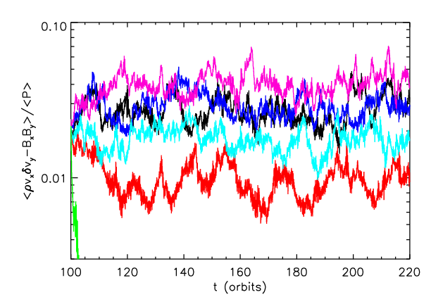
Figure 2: Volume-averaged total stress normalized by the the volume-averaged gas pressure as a function of time in orbits in the unstratified, toroidal field FT simulations. The black line corresponds to $Rm=3200$ and $P_{\rm m}=4$, magenta is $Rm=6400$ and $P_{\rm m}=8$, green is $Rm=800$ and $P_{\rm m}=0.5$, light blue is $Rm=3200$ and $P_{\rm m}=2$, dark blue is $Rm=6400$ and $P_{\rm m}=4$, and red is $Rm=3200$ and $P_{\rm m}=0.5$. There is a clear increase in stress with increasing $P_{\rm m}$. For sufficiently low $Rm$, the turbulence decays.

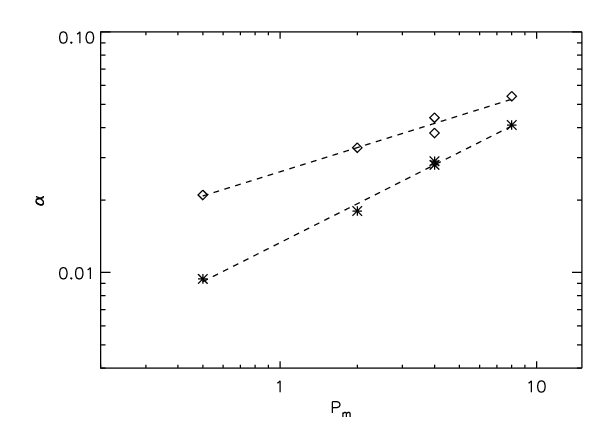
Figure 3: Time- and volume-averaged stress parameter $\alpha$ as a function of $P_{\rm m}$ in the unstratified FT simulations (asterisks) and the higher resolution, net toroidal field simulations of Simon & Hawley (2009) (diamonds). In the FT simulations, $\alpha\equiv\langle\langle\rho v_{x}\delta v_{y}-B_{x}B_{y}\rangle\rangle/\langle\langle P\rangle\rangle$, whereas in the higher resolution simulations, $\alpha\equiv\langle\langle\rho v_{x}\delta v_{y}-B_{x}B_{y}\rangle\rangle/P_{o}$; see Simon & Hawley (2009). These definitions are roughly equivalent since $\langle P\rangle\approx P_{o}$. For the FT simulations, the average is calculated over the entire simulation domain and from 120 orbits to the end of the simulation. Only simulations with sustained turbulence are plotted. The dashed lines are linear fits to the data in log-log space. Both resolutions show a clear $P_{\rm m}$ dependence, but this dependence is steeper at the lower resolution.

Next, we explore the influence of physical dissipation terms on the FT initial field configuration, using 32 zones per $H$. The time history of the volume-averaged stress for these runs is displayed in Fig. 2. There is a clear dependence on the dissipation parameters and on $P_{\rm m}$ in particular. For large enough resistivity (i.e., low $Rm$), the turbulence decays; the critical $Rm$ value is $\sim 1000$, in agreement with the higher resolution simulations of Simon & Hawley (2009). In Fig. 3, we plot the time-averaged $\alpha$ values, averaged from orbit 120 to the end of the simulation, versus $P_{\rm m}$ for these runs (asterisks). Note that 32FTRm3200Pm4 and 32FTRm6400Pm4 have different $Rm$ values, but the same $P_{\rm m}$ and nearly the same saturation level. We also plot $\alpha$ from the higher resolution simulations of Simon & Hawley (2009) (see their Table 3). The dashed lines are linear fits to the data in log-log space. Assuming $\delta$ in $\alpha\propto P_{\rm m}^{\delta}$ we find $\delta=0.54$ for 32 grid zones per $H$, and $\delta=0.33$ for 128 grid zones per $H$; the $P_{\rm m}$ dependence is steeper at the lower resolution. Furthermore, all of the $\alpha$ values for the higher resolution simulations are larger than the corresponding lower resolution simulations.

Both the zero net flux and net toroidal flux results suggest that moderate resolutions, i.e., 32 grid zones per $H$, may be sufficient to capture the general effects of changing $\nu$ and $\eta$, at least for the range of $Re$, $Rm$, and $P_{\rm m}$ values considered here. This is not to say that everything is converged at this resolution. Indeed, Fig. 3 shows a noticeable resolution effect. Full convergence likely requires a sufficiently high resolution to ensure that the effective numerical dissipation scale is below the viscous and resistive dissipation scales (see e.g., Fromang et al., 2007; Simon et al., 2009; Simon & Hawley, 2009), but the general dependence of $\alpha$ on dissipation parameters appears to be captured even at 32 zones per $H$. This conclusion is also supported by the recent results of Flaig et al. (2010), which show that $\sim 30$ zones per $H$ in the vertical direction may be sufficient to characterize the turbulence in their stratified shearing box simulations. This is an important point, as available computational resources limit us to this resolution in carrying out the comprehensive study of physical dissipation effects presented in this work.

3.2 Dissipation and Initial Field Strength

Because the fastest growing MRI wavelength is proportional to $v_{\rm A}$, the background field strength can play a significant role in the outcome of a shearing box simulation. For example, Longaretti & Lesur (2010) found that the dependence of angular momentum transport on $Rm$ and $P_{\rm m}$ becomes steeper for weaker background (vertical) fields in unstratified shearing boxes.

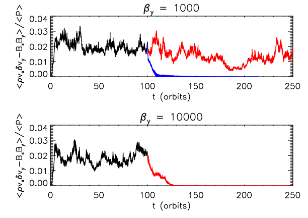
Figure 4: Volume-averaged total stress normalized by the volume-averaged gas pressure as a function of time in orbits for a series of unstratified shearing box simulations. The volume-average is done over the entire simulation domain. In each plot, the black line is from a simulation with only numerical dissipation. The colored lines are simulations with physical dissipation, initiated from the numerical dissipation run at orbit 100. The red lines correspond to $Rm=3200$, $P_{\rm m}=2$ and the blue line is $Rm=1600$, $P_{\rm m}=1$. The top panel is initiated with a background toroidal field characterized by $\beta=1000$, and the bottom panel has $\beta=10000$. The weaker toroidal field appears to be killed off at a lower resistivity compared to the stronger background field.

Here we consider the effects of different toroidal field strengths on the FT initial condition in the unstratified shearing box. We consider $\beta_{y}=1000$ and $\beta_{y}=10000$ runs both with and without physical dissipation (see Table 1 and § 2). The time history of the volume-averaged stresses for these simulations is shown in Fig. 4. For $\beta_{y}=1000$, the turbulence survives at $Rm=3200$ but dies at $Rm=1600$, whereas for $\beta_{y}=10000$, the turbulence dies at $Rm=3200$. It would seem that for each increase in $\beta_{y}$ by a factor of 10, the critical $Rm$ value increases by roughly a factor of 2; it becomes easier to kill off the MRI with a lower resistivity as the background toroidal field is weakened.

The time- and volume-averaged Elsasser numbers, calculated via equation (8), are 2.3 and 137 for the $\beta=1000$, $Rm=1600$ and 3200 models respectively. The time average is from orbit 140 to the end of the calculation, and since the turbulence decays, the average $\Lambda$ for $Rm=1600$ agrees with that given by the initial toroidal field value. For the $\beta=10000$, $Rm=3200$ model, the Elsasser number is 0.45, again, calculated from either the initial toroidal field strength or from equation (8) after the turbulence has completely decayed. In both cases the initial poloidal field has $\beta_{p}=1600$, corresponding to an initial poloidal $\Lambda$ on order unity for these $Rm$ values. These results are consistent with the $\Lambda$ values calculated in Simon & Hawley (2009); $\Lambda\lesssim 100$ leads to decay.

The time- and volume-averaged $Q_{y}$ values are $Q_{y}=34$ and $Q_{y}=33$ for 32FTNum$\beta$1000 and 32FTNum$\beta$10000, respectively. The time average is done from orbit 20 to 110. The toroidal field MRI appears to be quite well-resolved in both simulations. Averaging over the same time interval, we find that $Q_{z}=7.3$ for 32FTNum$\beta$1000 and $Q_{z}=6.9$ for 32FTNum$\beta$10000; the vertical field MRI is marginally resolved. Note that these $Q$ values are calculated via the saturated state of these runs. Indeed, the initial $Q$ values are substantially lower and either marginally or under-resolved. It is not clear which $Q$ values are a better representation of how well-resolved the MRI actually is; the initial values correspond to the background field which ultimately drives the MRI, but other modes may become important in driving the MRI in the fully nonlinear state. In any case, despite the low initial $Q$ values, sustained turbulence develops when explicit dissipation terms are not included, suggesting that at least some MRI modes are resolved. It is only when resistivity is turned on that decaying turbulence is observed. The initial low $Q$ values may introduce uncertainty for the specific values of the critical resistivity, but the relationship between critical resistivity and initial field strength is likely to hold nevertheless.

4 Vertically Stratified Simulations

4.1 Baseline Simulations

We now turn to a series of simulations that investigate the effects of physical dissipation in vertically stratified, isothermal disks. The various combinations of runs are summarized in Table 2. Some time- and volume-averaged values of various quantities are given in Table 3. The baseline calculations without physical dissipation are done at two resolutions: 32Num which uses 32 grid zones per $H$, and 64Num which uses 64. 32Num is run to a total integration time of 1058 orbits. It has sustained turbulence at a level of $\alpha=0.028$, calculated via equation (18), time-averaging from orbit 20 until the end of the calculation, and volume-averaging over all $x$ and $y$ and for $|z|\leq 2H$. In Model 64Num, $\alpha=0.022$, where the time average is from orbit 20 until the end of the simulation at 159 orbits.

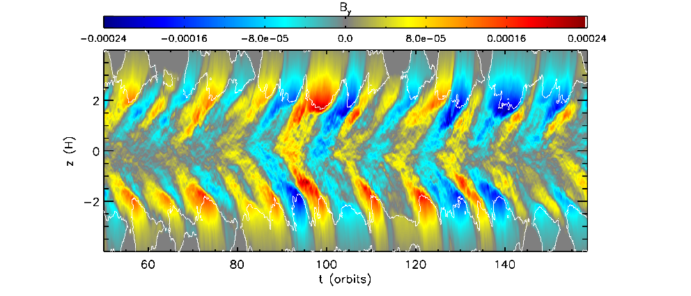
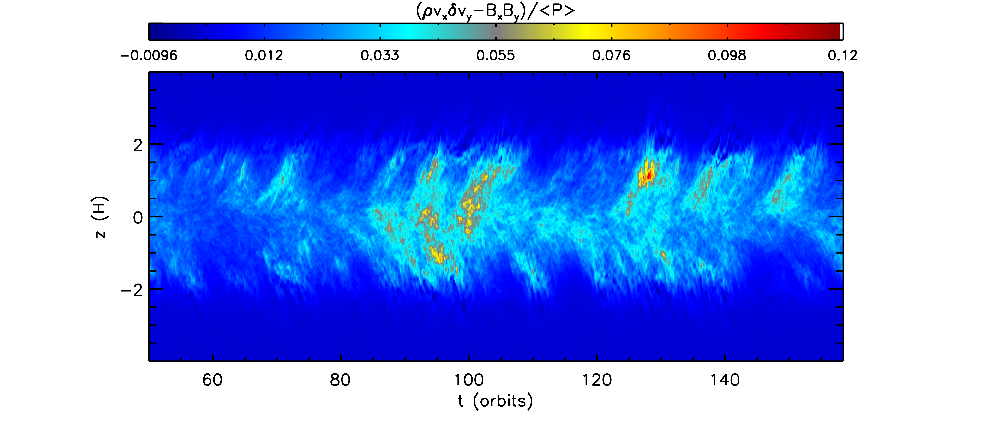
Figure 5: Space-time diagram of the horizontally averaged $B_{y}$ (top panel) and total stress normalized by the volume-averaged gas pressure (bottom panel). The volume-average is done for all $x$ and $y$ and for $|z|\leq 2H$. The white contours on the top panel denote where $\beta$ goes from greater to less than unity. The horizontally averaged $B_{y}$ appears to rise vertically into the upper $z$ layers, being replaced in the mid-plane region by $B_{y}$ of the opposite sign. The rise speed of the field increases after $|z|\sim 2H$ is reached. The sign flipping in $B_{y}$ has a period of $\sim 10$ orbits.

One particularly useful diagnostic is the space-time diagram of horizontally averaged quantities. Figure 5 shows space-time plots of horizontally averaged $B_{y}$ and pressure-normalized total stress for a 100 orbit period in the 64Num simulation. From this, we see that $B_{y}$ changes sign periodically and rises above the equatorial plane. The behavior of $B_{y}$ is roughly mirror symmetric around the equator and has a period of $\sim 10$ orbits at both resolutions. This has been seen in previous vertically stratified shearing boxes (e.g., Brandenburg et al., 1995; Stone et al., 1996; Hirose et al., 2006; Guan & Gammie, 2010; Shi et al., 2010; Gressel, 2010; Davis et al., 2010), with a variety of initial fields, numerical resolutions and codes, and it has even been observed in global simulations (e.g., Fromang & Nelson, 2006; Dzyurkevich et al., 2010; O’Neill et al., 2010). It is apparently a generic property of MRI-driven turbulence in the presence of vertical gravity.

The white contours in the top panel of Fig. 5 indicate where the gas $\beta$ value switches from greater than to less than unity. For $|z|\gtrsim 2-2.5H$, $\beta<1$, except for some regions very near the vertical boundaries where $\beta>1$ as a result of the absence of magnetic field. The region around $|z|=2H$ is also where the fluid becomes completely buoyantly unstable. Using the criterion of Newcomb (1961) as outlined in Guan & Gammie (2010), the gas is buoyantly stable if

$$\left|\frac{d\rho}{dz}\right|>\left|\frac{\rho^{2}g}{\gamma P}\right|$$ (19)

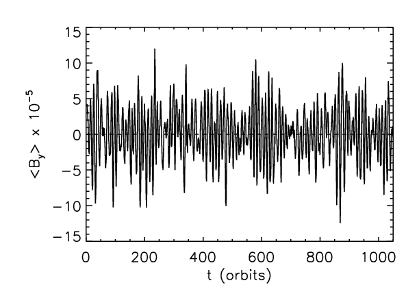
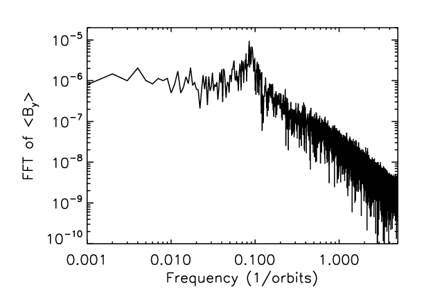
Figure 6: Left: Time evolution of volume-averaged $B_{y}$ in 32Num. The volume average is done for all $x$ and $y$ and for $|z|\leq 0.5H$. The dashed line corresponds to $\langle B_{x,y}\rangle=0$. Right: Temporal power spectrum of $\langle B_{y}\rangle$ from the left plot, calculated from orbit 50 to 1050. The 10 orbit period oscillations in $\langle B_{y}\rangle$ are immediately apparent in both plots, particularly as the peak in the power spectrum. The 10 orbit oscillations are modulated on longer timescales, ranging from tens to hundreds of orbits.

where $\gamma=1$ because the gas is isothermal. According to this criterion applied to the simulation data, the fluid is buoyantly unstable for $|z|\gtrsim 2H$. Consistent with this, the space-time plot shows that the field rises faster for $|z|\gtrsim 2H$. For $|z|\lesssim 2H$, there are regions of instability as well as stability, and it is within this region that the MRI is active as indicated by the presence of significant stress. Indeed, the total stress drops off rapidly near $|z|\sim 2H$. It appears that the marginal buoyancy stability coupled with the MRI-induced turbulence leads to a slower rise of magnetic field until $|z|\sim 1.5$–$2H$, where the gas then becomes completely buoyantly unstable. These results are consistent with the recent ZEUS calculations of Guan & Gammie (2010) with large radial extent as well as with Shi et al. (2010) using a version of ZEUS that includes radiation physics and total energy conservation. Compare, e.g., the top panel of Fig. 5 to Fig. 6 in Shi et al. (2010).

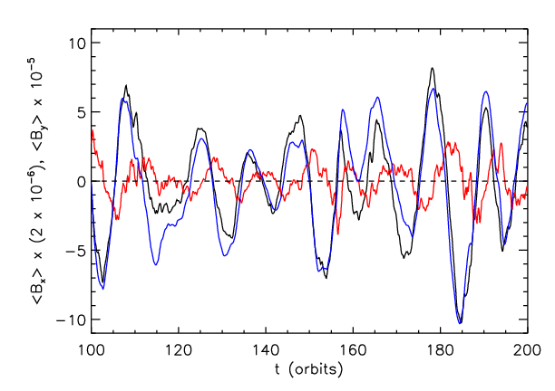
Figure 7: Time evolution of volume-averaged field components for part of 32Num. Red is $\langle B_{x}\rangle$, black is $\langle B_{y}\rangle$, and blue is $\langle B_{y}\rangle$ as calculated from $\langle B_{x}\rangle$ using a simple $\alpha$–$\Omega$ dynamo model discussed in the text. The volume average is done for all $x$ and $y$ and for $|z|\leq 0.5H$. The dashed line corresponds to $\langle B_{x,y}\rangle=0$. $\langle B_{x}\rangle$ has been multiplied by a factor of 5 relative to $\langle B_{y}\rangle$ to make a more direct comparison possible. The variations in $\langle B_{x}\rangle$ are accompanied by variations in $\langle B_{y}\rangle$, which are offset in time, and the dynamo model shows that the evolution of $\langle B_{y}\rangle$ is controlled by shear of radial field and buoyant removal of toroidal field.

Figure 6 shows the volume-averaged toroidal field within $|z|\leq 0.5H$ as a function of time. The RMS field fluctuations averaged within this region are roughly a factor of $\sim 4$ times larger; the turbulent fluctuations dominate over the mean, but not significantly so. The temporal oscillations in the mean field are apparent. The right figure shows the temporal power spectrum, revealing the dominant $\sim 10$ orbit period. The oscillation amplitude appears to be modulated on longer timescales, ranging from tens to hundreds of orbits. Furthermore, the averaged radial field appears to exhibit the same 10 orbit cyclic behavior as the toroidal field, but with a slight temporal lag, as shown in Fig. 7. The behavior of the mean radial and toroidal fields resembles the $\alpha$–$\Omega$ dynamo model derived in Guan & Gammie (2010). Specifically, they write simplified evolution equations for volume-averaged field components,

$$\frac{d\langle B_{y}\rangle}{dt}=-q\Omega\langle B_{x}\rangle-\frac{|v_{\rm A}|}{2H}\langle B_{y}\rangle+\frac{\alpha_{1}}{2H}\langle B_{x}\rangle,$$ (20)

$$\frac{d\langle B_{x}\rangle}{dt}=-\frac{|v_{\rm A}|}{2H}\langle B_{x}\rangle-\frac{\alpha_{2}}{2H}\langle B_{y}\rangle.$$ (21)

The first term on the right hand side of equation (20) is the background shear acting on the radial field. The second term is the loss of toroidal field due to buoyant rise, estimated to have a characteristic buoyant velocity equal to the toroidal field ${\rm Alfv\acute{e}n}$ speed. The third term is the $\alpha$-dynamo term coupling $B_{x}$ to the evolution of $B_{y}$. Equation (21) is similar except there is no shear term and the toroidal and radial field components have been flipped with respect to equation (20). Also, in general, $\alpha_{1}\neq\alpha_{2}$. Note that while we follow the notation and general approach of Guan & Gammie (2010) here, Gressel (2010) has also constructed an $\alpha$–$\Omega$ model, which incorporates a helicity-based dynamo mechanism and reproduces the observed behavior of the horizontally averaged field components.

Guan & Gammie (2010) numerically integrated this set of equations and found a solution that looks strikingly similar to the red and black curves in Fig. 7. The value of $\alpha_{1,2}$ sets the oscillation frequency in the mean field; $\alpha_{1}=\alpha_{2}=-0.01\Omega H$ reproduces the 10 orbit variability observed in stratified shearing boxes. Here we numerically integrate equation (20) using the simulation data for $\langle B_{x}\rangle$ (the red curve) and the initial condition for $\langle B_{y}\rangle$ taken from $\langle B_{y}\rangle$ at $t=0$. We have set $\alpha_{1}=0$ so that the $\langle B_{y}\rangle$ evolution is controlled entirely by shear and buoyancy. The result is the blue curve in the figure. The agreement between the actual evolution of $\langle B_{y}\rangle$ and the $\alpha$–$\Omega$ dynamo model suggests that the evolution of the mean toroidal field within the mid-plane region is almost completely controlled by the shearing of radial field and the buoyant removal of the generated toroidal field.

The remaining question then is, what creates the mean radial field? In the dynamo model, the $\alpha_{2}$ term is essential, but what mechanism is responsible for $\alpha_{2}\neq 0$? The most likely candidate is MRI turbulence; turbulent fluctuations create EMFs that generate poloidal field (e.g., Brandenburg et al., 1995; Davis et al., 2010; Gressel, 2010), but the details of this are still not well understood.

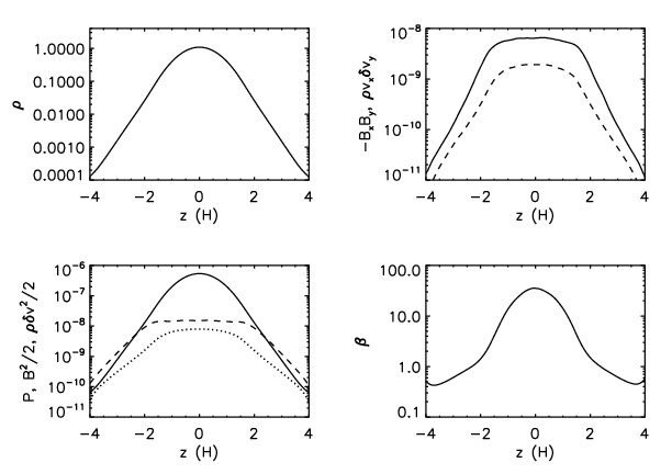
Figure 8: Time- and horizontally-averaged vertical distributions for various quantities in 32Num. Upper left: gas density; upper right: Maxwell (solid) and Reynolds (dashed) stresses; lower left: gas pressure (solid), magnetic energy (dashed), and kinetic energy (dotted); lower right: gas $\beta$ defined as the time- and horizontally-averaged gas pressure divided by the time- and horizontally-averaged magnetic energy density. The time average is done from orbit 100 to the end of the simulation. The stress and magnetic energy are relatively flat for $|z|\lesssim 1.5H$ but drop off substantially for larger $|z|$. Outside of $|z|\sim 2H$, the magnetic energy dominates over gas pressure.

In Fig. 8, we plot the time- and horizontally-averaged vertical distributions for various quantities in 32Num. The time average runs from orbit 100 to the end of the calculation. The figure shows that the stress drops off rapidly near $|z|\sim 1.5H$. The shape of the distribution is generally the same for both Maxwell and Reynolds stresses, with the Maxwell stress always greater than the Reynolds stress by a factor that varies from 2.3 to 5.6 depending on $z$; this factor is $\sim 4$ when averaged over all $z$, in agreement with unstratified simulations (e.g., Hawley et al., 1995). The gas pressure maintains an approximately Gaussian distribution consistent with hydrostatic equilibrium, while the magnetic pressure is subthermal and relatively flat for all $|z|\lesssim 2H$. The magnetic field becomes superthermal for $|z|>2H$, although its magnitude continues to decrease with height. These results are consistent with previous studies of isothermal disks (e.g., Stone et al., 1996; Miller & Stone, 2000; Guan & Gammie, 2010). Interestingly, the vertical structure of the turbulence is also consistent with local simulations containing radiation physics Hirose et al. (2006); Krolik et al. (2007); Hirose et al. (2009); Flaig et al. (2010) and global simulations Hawley et al. (2001); Fromang & Nelson (2006), though we do not observe the double peak profile in the stress as seen in the simulations of Hirose et al. (2009) and Flaig et al. (2010).

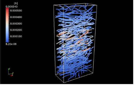
Figure 9: Magnetic field structure at $t=100$ orbits in 32Num, produced via a stream line integration. The field strength (in code units) is displayed via color and not the density of the field lines. The magnetic field has a primarily toroidal structure but has a smaller, tangled structure in the $x$ and $z$ directions.

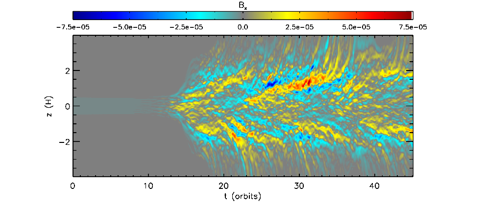
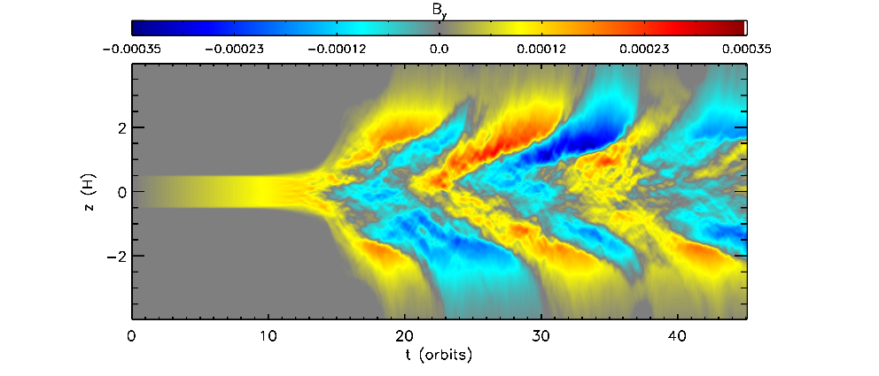
Figure 16: Space-time diagram of the horizontally averaged $B_{x}$ (top panel) and $B_{y}$ (bottom panel) for 32ShearBx. The uniform radial field that is present initially shears into toroidal field, which eventually becomes strong enough to launch the MRI.

Figure 9 examines the three-dimensional structure of the magnetic field in the fully turbulent gas using streamline integration for 32Num at $t=100$ orbits. The field strength is denoted by color rather than field line density. Within $|z|\lesssim 2H$, the field is primarily toroidal but has a smaller scale, tangled structure in the $x$ and $z$ directions. Very near the vertical boundaries, however, the field appears to develop larger poloidal components. Utilizing snapshots taken throughout the evolution of 32Num, we find that this is typical of the saturated state, except for at $t=550$ orbits, in which the field near the boundaries is primarily vertical. Figure 16 of Hirose et al. (2006) shows the field in a shearing box with a vertical domain twice as large as 32Num. In their simulation, the field at $|z|=4H$ is mainly toroidal while the field structure at $|z|=4H$ in 32Num resembles the field structure near $|z|=8H$ in their simulation. This suggests that the vertical outflow boundary conditions are influencing the field structure very near the boundaries. Away from the vertical boundaries, however, the magnetic field in 32Num appears to have a very similar structure to that in Hirose et al. (2006).

Table 3: Saturation Characteristics for Sustained Turbulence Runs

Quantity	32Num	32Rm3200Pm4	32Rm6250Pm1	32Rm6400Pm4	32Rm6400Pm8	64Num	64Rm3200Pm2	64Rm6400Pm4
$\langle\langle-B_{x}B_{y}\rangle\rangle/\langle\langle P\rangle\rangle$	0.022	0.023	0.018	0.025	0.033	0.018	0.027	0.025
$\langle\langle\rho v_{x}\delta v_{y}\rangle\rangle/\langle\langle P\rangle\rangle$	0.0058	0.0051	0.0046	0.0061	0.0071	0.0044	0.0060	0.0055
$\langle\langle B^{2}/2\rangle\rangle/\langle\langle P\rangle\rangle$	0.059	0.069	0.050	0.069	0.089	0.045	0.074	0.063
$\langle\langle B_{x}^{2}/2\rangle\rangle/\langle\langle P\rangle\rangle$	0.0066	0.0059	0.0051	0.0069	0.0084	0.0061	0.0079	0.0072
$\langle\langle B_{y}^{2}/2\rangle\rangle/\langle\langle P\rangle\rangle$	0.049	0.060	0.043	0.058	0.077	0.036	0.062	0.052
$\langle\langle B_{z}^{2}/2\rangle\rangle/\langle\langle P\rangle\rangle$	0.0031	0.0028	0.0024	0.0032	0.0039	0.0030	0.0040	0.0035
$\langle\langle\rho\delta v^{2}/2\rangle\rangle/\langle\langle P\rangle\rangle$	0.024	0.021	0.020	0.024	0.027	0.020	0.025	0.022
$\langle\langle\rho v_{x}^{2}/2\rangle\rangle/\langle\langle P\rangle\rangle$	0.010	0.0088	0.0085	0.010	0.011	0.0079	0.010	0.0094
$\langle\langle\rho\delta v_{y}^{2}/2\rangle\rangle/\langle\langle P\rangle\rangle$	0.0079	0.0066	0.0062	0.0078	0.0089	0.0070	0.0084	0.0075
$\langle\langle\rho v_{z}^{2}/2\rangle\rangle/\langle\langle P\rangle\rangle$	0.0059	0.0057	0.0052	0.0061	0.0068	0.0047	0.0065	0.0055
$\langle\langle-B_{x}B_{y}\rangle\rangle/\langle\langle\rho v_{x}\delta v_{y}\rangle\rangle$	3.77	4.55	3.87	4.18	4.58	4.03	4.47	4.60
$\langle\langle-B_{x}B_{y}\rangle\rangle/\langle\langle B^{2}/2\rangle\rangle$	0.37	0.34	0.36	0.37	0.37	0.40	0.36	0.40

4.2 High and Low Turbulence States

Having established the baseline simulations without physical dissipation, we now turn to the main focus of our present work: the effect of $\nu$ and $\eta$ on vertically stratified MRI turbulence.

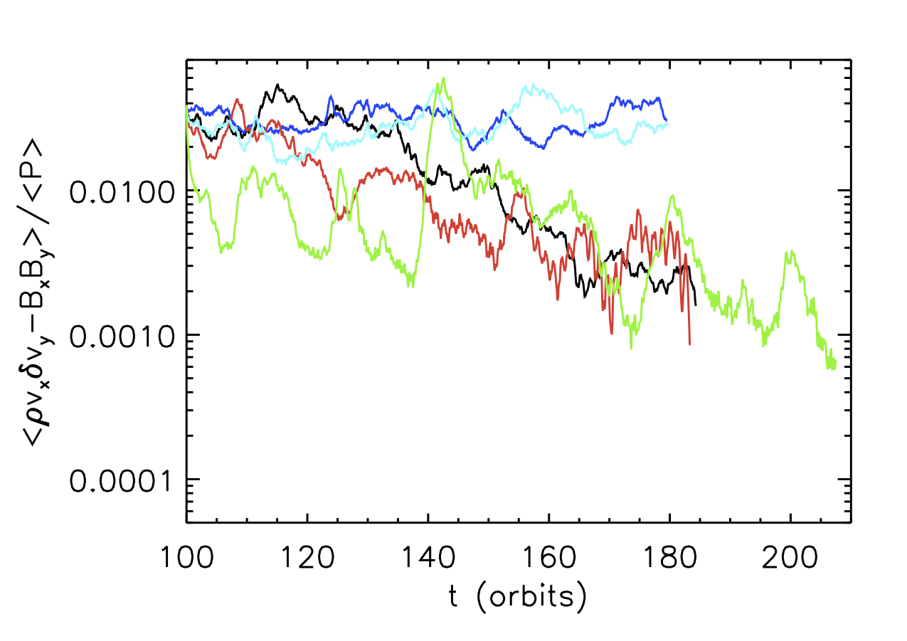
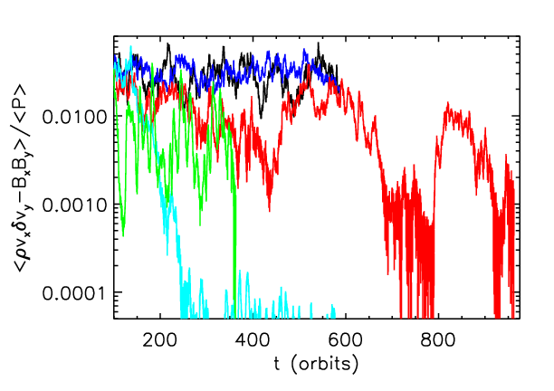
Figure 10: Volume-averaged total stress normalized by the volume-averaged gas pressure as a function of time in orbits in the vertically stratified simulations at 64 (left) and 32 (right) grid zones per $H$. The volume-average is done for all $x$ and $y$ and for $|z|\leq 2H$. The black line corresponds to $Rm=3200$ and $P_{\rm m}=4$, green is $Rm=800$ and $P_{\rm m}=0.5$, light blue is $Rm=3200$ and $P_{\rm m}=2$, dark blue is $Rm=6400$ and $P_{\rm m}=4$, and red is $Rm=3200$ and $P_{\rm m}=0.5$. Some of the simulations appear to undergo periods of low stress followed by higher stress, occurring on very long timescales of $\sim 100$ orbits in some cases.

The Maxwell and Reynolds stress time evolution for the simulations performed with 64 zones per $H$ is shown in the left panel of Fig. 10. Runs 64Rm3200Pm0.5, 64Rm800Pm0.5, and 64Rm3200Pm4 have decreasing turbulence levels, while turbulence is sustained at a statistically constant value in the remaining simulations. Furthermore, 64Rm800Pm0.5 undergoes alternating periods of low and high stress, though the overall trend is downward with time.

The right panel of Fig. 10 is the stress evolution for the equivalent simulations with 32 zones per $H$, shown for a much longer time period than the 64 zone runs. There is considerable variability on long timescales. 32Rm3200Pm0.5 in particular exhibits alternating periods of low and high stress levels, occurring on $\sim 100-200$ orbit timescales. The more viscous and resistive run, 32Rm800Pm0.5, shows similar variability but on a much shorter timescale of $\gtrsim 10$ orbits. Turbulence in 32Rm3200Pm2 appears to have leveled off at a smaller value without any indication of regrowth to the higher state. Both 32Rm6400Pm4 and 32Rm3200Pm4 remain at relatively high stress levels, which are very similar between the two runs, likely a result of having the same $P_{\rm m}$.

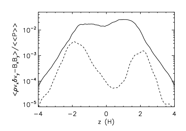
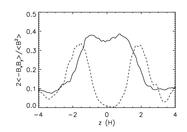
Figure 11: Left: Time- and horizontally-averaged total stress as a function of $z$ for 32Rm3200Pm0.5. The stress is normalized by the time- and volume-averaged gas pressure, where the volume average is done for all $x$ and $y$ and for $|z|\leq 2H$. Right: Ratio of time- and horizontally-averaged Maxwell stress to time- and horizontally-averaged magnetic energy in 32Rm3200Pm0.5. In both plots, the solid line corresponds to a time average from 500 to 570 orbits, which is a state of high turbulence, and the dashed line is a time average from 700 to 770 orbits, a low turbulence state. During the high state, the stress is relatively flat for $|z|\leq 2H$. In the low state, the stress is smaller within the mid-plane region and peaks near $|z|\sim 2H$.

Turning to the high and low states in 32Rm3200Pm0.5, the left panel of Fig. 11 shows the vertical profile for the horizontally averaged total stress during a high turbulence state (solid line, time averaged from 500 to 570 orbits) and a low turbulence state (dashed line, time averaged from 700 to 770 orbits). The high state has considerable stress within the mid-plane region ($|z|\lesssim 2H$), whereas in the low state, the stress is peaked near $|z|\sim 2H$. Note that there is still a nonzero stress in the mid-plane region even during the low state. The Reynolds stress is nonzero and relatively flat throughout the mid-plane, whereas the Maxwell stress drops off dramatically at the mid-plane. What Maxwell stress is present in the low states seems to derive from the presence of residual radial and toroidal field. (This effect was also noted by Turner et al. (2007) in the dead zone regions of their shearing box calculations). One characteristic of MRI turbulence is the ratio of the Maxwell stress to the magnetic pressure, which is typically on order 0.4 (Hawley et al., 1995; Blackman et al., 2008, and Table 3). The vertical profile of this ratio is shown in the right panel of Fig. 11. This ratio is between 0.3 and 0.4 for $|z|\lesssim 1.5H$ in the high state and near $|z|\sim 2H$ in the low state; in the mid-plane region during the low state, the ratio is much smaller and approaches zero.

These differences between the high and low states are seen in the other simulations that exhibit this variability (except for 32Rm800Pm0.5, in which the variability occurs on such a short timescale that temporal averaging becomes difficult). In summary, during the high state, the MRI is fully active, producing turbulent stresses for $|z|\lesssim 2H$. In the low state, the turbulence in the mid-plane region has died down, leaving weaker Reynolds stresses. MRI-driven turbulence is present, however, in narrow regions near $|z|\sim 2H$. This is similar to the behavior seen in Fleming & Stone (2003) where active layers above and below the mid-plane drive Reynolds stresses in the equatorial dead zone.

Is the variability between high and low turbulence an artifact of using a relatively low resolution in these calculations? Several pieces of evidence suggest this is not the case. First of all, both resolutions for $Re=1600$, $P_{\rm m}=0.5$ show the same variable stress behavior on $\gtrsim 10$ orbit timescales. Secondly, even at 32 zones per $H$, dissipation coefficients play a significant role in determining the stress level, as shown above. The fact that the low resolution, unstratified simulations show constant saturation levels for sufficiently small $\eta$ whereas vertically stratified simulations exhibit this variability for the same parameters suggests that the variability is a direct result of adding in vertical gravity. Thirdly, this variability was seen in the simulations of Davis et al. (2010), which were run at a higher resolution of 64 zones per $H$. We note, however, that while Davis et al. (2010) used the same numerical algorithm as in this work, they used a different initial magnetic field configuration and vertical boundary conditions.

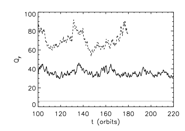
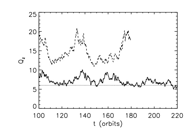
Figure 12: Quantitative measurement of how well resolved the MRI is in the toroidal ($Q_{y}$; left plot) and vertical ($Q_{z}$; right plot) directions as a function of time. The solid line corresponds to run 32Rm6400Pm4 and the dashed line is 64Rm6400pm4. The dotted horizontal line corresponds to $Q=6$, below which the MRI is considered to be under-resolved Sano et al. (2004). $Q_{i}$ is calculated using the volume average of the magnetic energy and gas density for all $x$ and $y$ and for $|z|\leq 0.5H$ (see text). The toroidal field MRI at both resolutions as well as the vertical field MRI at the higher resolution appear to be reasonably well-resolved. However, at the lower resolution, the vertical field MRI is only marginally resolved.

Finally, we examine the $Q$ values (10) using an ${\rm Alfv\acute{e}n}$ speed defined by (9) and a volume average for all $x$ and $y$ and for $|z|\leq 0.5H$. Figure 12 shows $Q_{y}$ and $Q_{z}$ as a function of time for 32Rm6400Pm4 and 64Rm6400pm4. The results suggest that the toroidal field MRI is quite well-resolved, but that the vertical field MRI may be only marginally resolved for the lower resolution simulation. The higher resolution $Q$ values are roughly a factor of 2 larger than the lower resolution $Q$ values, which is simply a result of the change in the grid zone size; the turbulent saturation level is roughly the same between the two resolutions. This result, coupled with the somewhat low $Q_{z}$ value, suggests that the vertical field MRI may not be playing a particularly significant role in setting the saturation level in these simulations.

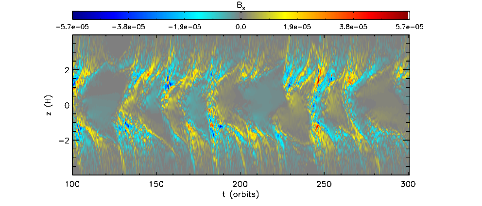
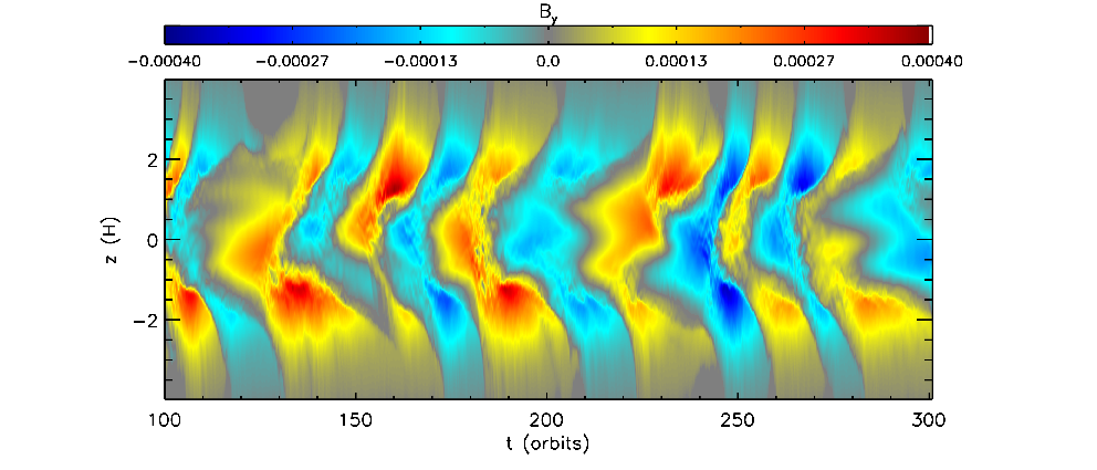
Figure 13: Space-time diagram of the horizontally averaged $B_{x}$ (top panel) and $B_{y}$ (bottom panel) for the first 200 orbits of 32Rm800Pm0.5. The turbulence initially decays, leaving a net $B_{x}$ within the mid-plane region, which shears into toroidal field. This appears to eventually reenergize the MRI, but the large resistivity quickly quenches the turbulence again.

If this high-low variability is indeed a physical effect, what is its origin? First, consider the space-time diagram of the horizontally averaged $B_{x}$ and $B_{y}$ for several simulations. Figure 13 shows the first 200 orbits of 32Rm800Pm0.5. The turbulence level decreases dramatically from the beginning (see also Fig. 10). This is not too surprising considering that the same $Rm$, $P_{\rm m}$ values cause rapid decay of the turbulence in the unstratified case; the resistivity is large enough to damp the MRI. The space-time plots show that after this decay, there is a residual magnetic field left within the mid-plane region of the disk. In particular, within $|z|\lesssim 0.5H$, there is a net horizontally averaged $B_{x}<0$ and $B_{y}<0$ around $t=110$ orbits. The average $B_{x}$ within this region remains constant for awhile, and $B_{y}$ increases due to the shear of $B_{x}$, eventually flipping to $B_{y}>0$. By $t\sim 130$ orbits, the turbulence has re-emerged, and the average $B_{y}$ rises to larger $|z|$. The resistivity then kills off the MRI again, leading to another period of $B_{x}$ shearing into $B_{y}$ before the next period of increased turbulence.

Model 32Rm3200Pm0.5 also experiences alternating high and low turbulence states, but it is not immediately clear why the turbulence within the mid-plane region should decay since the unstratified run with the same dissipation terms has sustained turbulence. As noted earlier and in Simon & Hawley (2009), the critical $Rm$ value below which the turbulence decays in unstratified shearing boxes is $\sim 1000$, but here $Rm=3200$. The major difference between the stratified and unstratified simulations is that with vertical gravity, the net magnetic field within a localized region of the domain can change due to buoyancy, whereas with unstratified boxes the net toroidal field remains constant. Loss of flux can raise the critical $Rm$ value (numerical resolution is also likely to have an effect); indeed, the unstratified simulations initialized with $\beta=1000$ and $\beta=10000$ fields have demonstrated that the critical $Rm$ depends upon the background field strength. The loss of net flux in a stratified box could similarly change the critical $Rm$ value.

In this simulation, the average toroidal field within the mid-plane region, $\langle B_{y}\rangle$, oscillates around zero with a period of 10 orbits. Thus, every 10 orbits or so, $\langle B_{y}\rangle$ is conceivably weak enough for resistivity to kill the turbulence. However, the turbulence remains for many of these 10 orbit periods. Furthermore, averaging $B_{y}$ within some vertical distance from the mid-plane erases information about the field structure there; e.g., $\langle B_{y}\rangle$ might be small but there could still be strong toroidal fields of opposite polarity close to $z=0$. The point is, one cannot necessarily expect the turbulence to decay away strictly whenever $\langle B_{y}\rangle$ drops below a certain (small) value.

The $\langle B_{y}\rangle$ oscillation amplitude appears to be modulated by a longer timescale, more on the order of $\sim 100$ orbits (see, e.g., Fig. 6). This behavior is present in all simulations with and without physical dissipation. This is also roughly the same timescale over which the system switches between low and high states in the $Rm=3200$ simulations. Comparing the time evolution of $\langle B_{y}\rangle$ for $|z|\leq 0.5H$ with the evolution of the total stress shows that the minima in the oscillation amplitude are generally correlated with the decay of mid-plane turbulence. One exception is near 200 orbits in 32Rm3200Pm0.5 in which $\langle B_{y}\rangle$ becomes rather small, but the turbulence remains active, though relatively weak compared to the fully active state. This correlation implies that if the mean toroidal field near the mid-plane remains sufficiently small for some time, resistivity can overwhelm the MRI and cause decay.

Evidently, there exists a critical $Rm$ below which the turbulence experiences long-timescale variability; this critical value is $Rm<6000$. We carry out two more stratified simulations with $Rm\sim 6000$ but different $P_{\rm m}$ values in order to further test this hypothesis. The first simulation is 32Rm6400Pm8; thus, $Rm=6400$, and $P_{\rm m}$ is relatively large. The mid-plane turbulence is sustained over a long time, nearly 330 orbits, without any sign of decay. The dissipation coefficients of the second simulation, 32Rm6250Pm1, are chosen to match the relatively high $Rm$, low $P_{\rm m}$ simulation that decays in the zero net flux shearing box (see Fromang et al., 2007; Simon & Hawley, 2009). This simulation also remains in the high state for nearly 330 orbits.

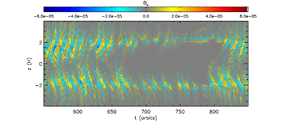
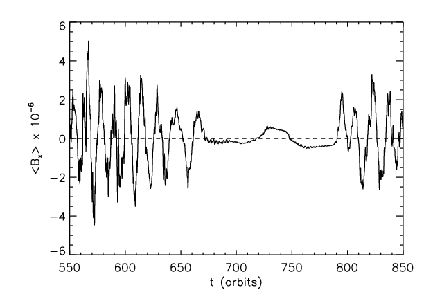
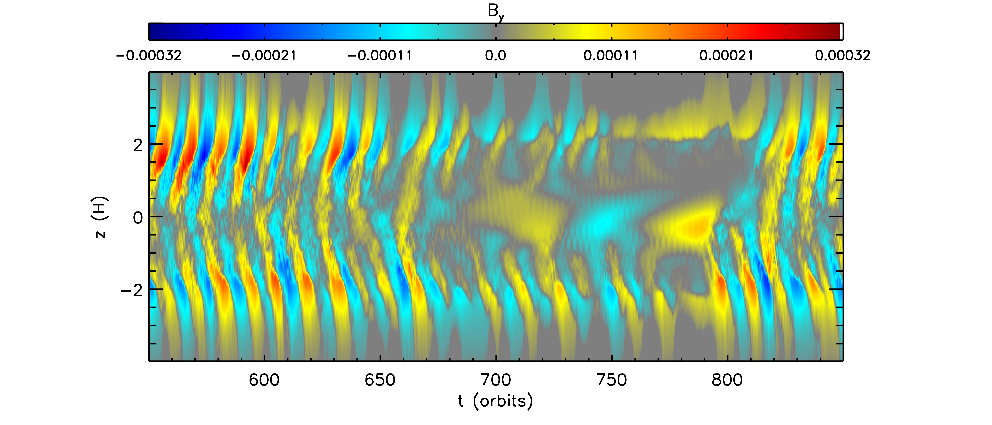
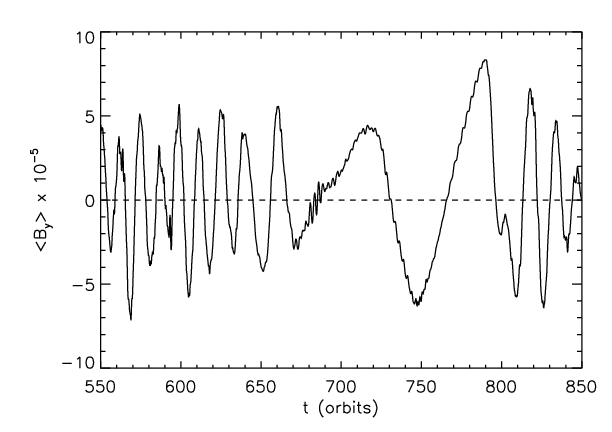
Figure 14: Space-time diagram of the horizontally averaged $B_{x}$ (top left) and $B_{y}$ (bottom left) for a 300 orbit period in 32Rm3200Pm0.5, and the average of $B_{x}$ (top right) and $B_{y}$ (bottom right) over all $x$ and $y$ and for $|z|\leq 0.5H$ as a function of time in orbits for the same 300 orbit period. During the period of no MRI turbulence, a net radial field still exists within the mid-plane region. This field appears to flip signs occasionally, leading to corresponding flips in $B_{y}$ due to shear.

If the dissipation is large enough to cause MRI-driven turbulence to decay, what leads to its reactivation after $\gtrsim 100$ orbits of time? Figure 14 shows the space-time plot of $B_{x}$ and $B_{y}$ for a 300 orbit period in 32Rm3200Pm0.5 during which the mid-plane turbulence dies out and eventually returns. For clarity, we also plot the volume-averaged horizontal field, $\langle B_{x}\rangle$ and $\langle B_{y}\rangle$, where the average is done for all $x$ and $y$ and for $|z|\leq 0.5H$. During the low state, there is a small net radial field that remains in the mid-plane region and generates $B_{y}$ through shear. The sign of the net $\langle B_{x}\rangle$ reverses and with it the sign of $\partial\langle B_{y}\rangle/\partial t$. The last such switch in the low state occurs around 750 orbits after which $\langle B_{y}\rangle$ continues to grow up until 790 orbits. At this point, the 10 orbit period oscillations resume.

Figures 13 and 14 suggest that it is the growth of $B_{y}$ due to shear that periodically reactivates the MRI in the mid-plane. Indeed, during the low states, the poloidal fields are sufficiently weak that the most unstable wavelengths of the radial and vertical field MRI are very under-resolved; $Q_{x}\lesssim 1$ and $Q_{z}\lesssim 1$ for both 32Rm800Pm0.5 and 32Rm3200Pm0.5. ($Q$ was calculated as a function of time using equations (9) and (10).) Considering the toroidal field, however, we find that $Q_{y}$ is well above the marginal resolution limit when the mid-plane turbulence starts to decay. In the low states of 32Rm800Pm0.5, $Q_{y}\sim 10-20$ occasionally dropping to $Q_{y}=6$. The typical $Q_{y}$ values for the low states of 32Rm3200Pm0.5 are similar but somewhat smaller. Of course when studying the behavior of the MRI in a situation where the $Q$ values are small, one is in a regime where numerical resolution is likely to matter. The specific behavior of the disk in the low state might be different at higher resolution, but shearing of radial into toroidal field is itself not so dependent on resolution. Thus, $Q$ may well play a role in determining when the MRI is reactivated, but not how it is reactivated.

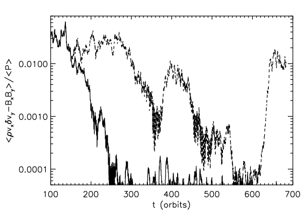
Figure 15: Volume-averaged total stress normalized by the volume-averaged gas pressure as a function of time in orbits in 32Rm3200Pm2 (solid line) and 32Rm3200Pm2_By+ (dashed line). The volume average is done over all $x$ and $y$ and for $|z|\leq 2H$. The run in which a net $B_{y}$ is added into the mid-plane region (dashed line) remains in the high state at first and then exhibits variability between low and high states.

As a further test, we carry out two additional experiments. First, we take the state of the gas in 32Rm3200Pm2 at $t=150$ orbits when the stress levels are decreasing and the average of $B_{y}$ within $|z|\leq 0.5H$, $\langle B_{y}\rangle=5.9\times 10^{-6}$, is relatively small compared to the oscillation amplitude of $\langle B_{y}\rangle$ in the high state, which is $\sim 5\times 10^{-5}$. We restart this simulation and add a net $B_{y}=8.9\times 10^{-5}$ into the region $|z|\leq 0.5H$, which corresponds to a toroidal $\beta\approx 126$ (using $\beta$ defined with the initial mid-plane gas pressure $P_{o}$). This run is 32Rm3200Pm2_By+ (see Table 2). Figure 15 shows the subsequent evolution of the stress along with the stress evolution of 32Rm3200Pm2. Not only does the mid-plane turbulence return, but the system undergoes episodic transitions between low and high states on $\sim 100$ orbit time scales, as in 32Rm3200Pm0.5.

In a second experiment, we initialize a stratified shearing box with all the same parameters as in 32Num but with an initially very weak radial magnetic field. Specifically, for $|z|\leq 0.5H$, $B_{x}=-\sqrt{2P_{o}/\beta_{x}}$ where $\beta_{x}=10^{6}$. This field strength is very under-resolved; the $Q_{x}$ value is 0.2, and the radial field MRI will not be significant. Figure 16 shows the space-time diagrams of horizontally averaged $B_{x}$ and $B_{y}$. The weak radial field is sheared into toroidal field that grows linearly in time until it reaches a sufficient strength to activate the MRI. The onset of MRI turbulence is rapid, and once the MRI sets in, the subsequent behavior is very similar to the other vertically stratified MRI simulations; there are rising magnetic field structures, dominated by the toroidal component, and the period of oscillations in the mean field is $\sim 10$ orbits. Note that this experiment is not an exact imitation of the low state in our simulations; there is no MRI activity near $|z|\sim 2H$ initially. However, this calculation demonstrates that shear amplification of a weak radial field can eventually lead to turbulence and move the system to the high state.

All of the simulations in which turbulence in the mid-plane sets in after a period of quiescence show the presence of a net radial field in the mid-plane during the low state. 32Rm3200Pm2, however, is the only simulation that does not show the re-emergence of the mid-plane MRI, despite over 1000 orbits of integration. An examination of the mid-plane region (up to $|z|\lesssim H$) in the low state of this run shows that the residual radial field is weaker than in the low states of the other simulations. If this radial field would remain constant in time, the toroidal field would continually strengthen to the point of reactivating the MRI. However, $\langle B_{x}\rangle$ continues to change sign even in the absence of turbulence, though with a period of many hundreds of orbits. That is, $\langle B_{x}\rangle$ oscillates about zero but with a very small amplitude. $\langle B_{y}\rangle$ similarly oscillates around zero and never reaches a sufficient amplitude to reactivate the MRI, and the simulation remains in the low state.

In fact, $\langle B_{x}\rangle$ oscillates about zero in all of our simulations, even in the low states (see e.g., Fig. 14). The various space-time diagrams suggest horizontal field migrates toward the mid-plane region from near $|z|\sim 2H$ where MRI activity is on-going. The oscillations in the mid-plane field components are a direct result of the oscillations previously observed in vertically stratified MRI turbulence. It is not entirely clear, however, what causes the field to migrate to the mid-plane. Does it diffuse there or is it carried downward by some sort of large scale flow? The shearing box calculations of Turner et al. (2007) and Turner & Sano (2008), which include Ohmic resistivity via a treatment of ionization chemistry, suggest that turbulent diffusion from the active layers is responsible for the field migration. While our simulations include a simpler prescription for resistivity, it is conceivable that a similar process is at work here. These issues will be addressed in future work.

To summarize the results for transitions between high and low states, we find that for sufficiently small $Rm$, MRI turbulence within the mid-plane region can decay away, in part because of loss of net flux due to buoyancy. Residual net radial field remains and subsequently creates toroidal field from shear. Once this toroidal field reaches a sufficiently large amplitude, the MRI is reactivated, and the turbulence is sustained for some duration until it decays again, repeating the pattern. In other words, the $\alpha$–$\Omega$ dynamo, seen in stratified simulations without resistivity, continues to operate in resistive simulations where the mid-plane MRI is suppressed. The dynamo is key to reactivation of MRI-driven turbulence.

This behavior appears to be independent of the $P_{\rm m}$ values we have used, except for near $Rm=3200$; 32Rm3200Pm4 remains in the high state, whereas 32Rm3200Pm2, 32Rm3200Pm2_By+, and 32Rm3200Pm0.5 do not. However, in the higher resolution runs, 64Rm3200Pm4 and 64Rm3200Pm0.5 show decay but 64Rm3200Pm2 appears to be sustained (though again, these simulations were not integrated very far). While $P_{\rm m}$ may play a role here, the line between sustained and highly variable stress levels is unlikely to be hard and fast, and many factors probably contribute to the nature of the turbulence near this $Rm$ value.

Comparing our results with those of Davis et al. (2010), we note that the largest $Rm$ used in their simulations was $Rm=3200$, consistent with the largest critical $Rm$ observed in our simulations. Secondly, an examination of the space-time data from their simulation with $Rm=1600$, $P_{\rm m}=2$ (kindly provided by the authors) shows the same behavior as we have observed here; a net radial field remains within the mid-plane region after decay, shearing into toroidal field, from which the MRI is reactivated within this region.

Interestingly, Turner et al. (2007) briefly notes that the toroidal field in the dead zone of some of their highly resistive simulations can occasionally become strong enough to reactivate turbulence there, after which the MRI is rapidly switched off again due to Ohmic dissipation. These simulations are consistent with our highest resistivity ($Rm=800$) simulations, in which turbulence occurs in short outbursts rather than through a transition to a long-lived high state, as is the case at lower resistivities.

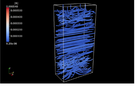
Figure 17: Magnetic field structure at $t=550$ orbits in 32Rm3200Pm2_By+, produced via a stream line integration. The field strength (in code units) is displayed via color and not the density of the field lines. The color scale is the same as that in Fig. 9 for comparison. This snapshot corresponds to the low state. The magnetic field is almost completely toroidal near the mid-plane but has a tangled structure in the upper $|z|$ regions, more reminiscent of the active state.

Lastly, we examine the topology of the magnetic field in the shearing box during the low state. Figure 17 shows the equivalent information as Fig. 9, but for orbit 550 of 32Rm3200Pm2_By+. For $|z|\gtrsim 2H$, the field remains mainly toroidal but with noticeable excursions from being purely toroidal, resembling the field structure in this region during the high state. Within $2H$, the field is almost completely toroidal, and any small poloidal field present within this region is not visible in this image. We also examined the azimuthally averaged poloidal field structure in several snapshots of this run. We found that the structure of the field was different, depending on which snapshot we examined. At some times, the poloidal field within $2H$ is almost completely radial, with very little vertical field. At other times, the vertical and radial fields are comparable in size such that the field takes on a more loop-like structure.

4.3 The Prandtl Number Effect on Sustained Turbulence

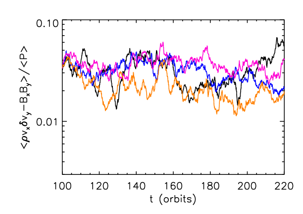
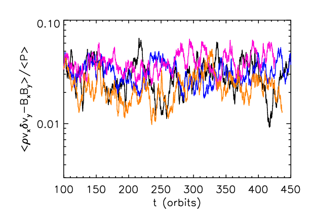
Figure 18: Volume-averaged total stress normalized by the volume-averaged gas pressure as a function of time in orbits in the lower resolution, vertically stratified simulations where turbulence remains sustained. The volume-average is done for all $x$ and $y$ and for $|z|\leq 2H$. The left plot is the first 120 orbits of the evolution, whereas the right plot is 350 orbits of the evolution. The black line corresponds to $Rm=3200$ and $P_{\rm m}=4$, dark blue is $Rm=6400$ and $P_{\rm m}=4$, magenta is $Rm=6400$ and $P_{\rm m}=8$, and brown is $Rm=6250$ and $P_{\rm m}=1$. The vertical axis has been chosen to match that of Fig. 2 for comparison. While the stress levels generally increase with $P_{\rm m}$, there is significant overlap between the different curves at different times.

In this section, we investigate how $P_{\rm m}$ affects angular momentum transport in simulations that do not exhibit the high-low variability. Figure 18 shows the volume-averaged stress levels for these simulations normalized by the gas pressure. The volume average is done for all $x$ and $y$ and for $|z|\leq 2H$. The figure shows a general increase in the turbulence levels with $P_{\rm m}$, but there is also significant time variability in the stress. As a result, the curves overlap at certain times, much more so than for unstratified turbulence (see Fig. 2).

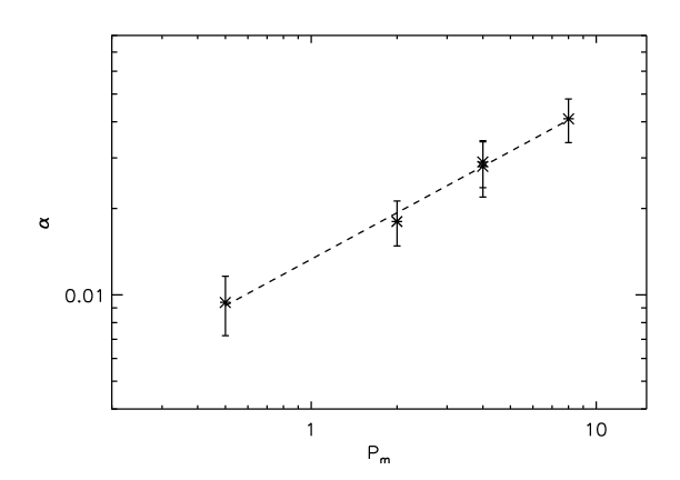
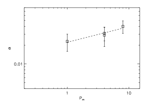
Figure 19: Time- and volume-averaged stress parameter $\alpha$ as a function of $P_{\rm m}$ in the unstratified FT simulations (left plot) and the stratified simulations (right plot); $\alpha~{}\equiv~{}\left\langle\langle\rho v_{x}\delta v_{y}-B_{x}B_{y}\rangle\rangle/\langle\langle P\rangle\right\rangle$. The average is calculated over the entire domain (all $x$ and $y$ and for $|z|\leq 2H$) and from 120 (150) orbits to the end of the simulation for the unstratified (stratified) runs. The dashed lines are linear fits to the data in log-log space, and the error bars denote one standard deviation about the temporal average of the numerator in $\alpha$. Both cases show a clear $P_{\rm m}$ dependence. However, in the stratified runs, this dependence is less steep, and there is considerable temporal variability.

Figure 19 displays the time-averaged $\alpha$ values as a function of $P_{\rm m}$ for the unstratified (left panel) and stratified simulations (right panel). The time average for the unstratified simulations is the same as in Fig. 3, from orbit 120 to the end of the calculation, and for the stratified simulations, this average is done from orbit 150 until the end of the simulation. The error bars denote one standard deviation about the temporal average of the numerator in $\alpha$. While there is a clear dependence of $\alpha$ on $P_{\rm m}$ in the stratified simulations, it is not as steep as in the unstratified simulations. Taking a linear fit in log-log space, and assuming $\alpha\propto P_{\rm m}^{\delta}$, $\delta=0.54$ for the unstratified runs (from § 3), and $\delta=0.25$ for the stratified calculations. In addition, the time variability is significantly larger in the stratified runs than in the unstratified case.

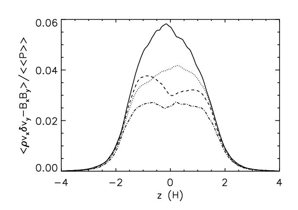
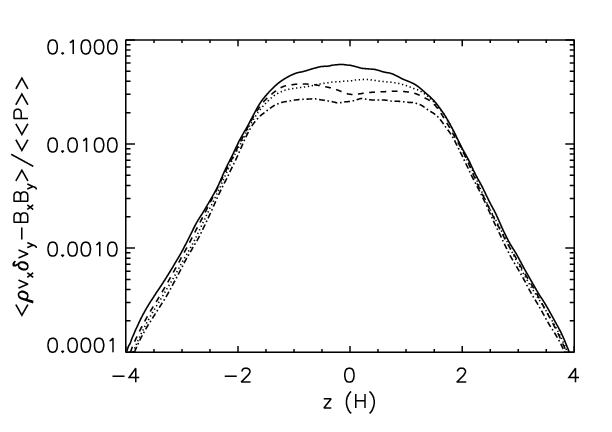
Figure 20: Time- and horizontally-averaged total stress as a function of $z$ on a linear (left) and logarithmic (right) vertical scale. The stress is normalized by the time- and volume-averaged gas pressure, where the volume average is done for all $x$ and $y$ and for $|z|\leq 2H$. The time average is done from orbit 150 until the end of each simulation. The solid line corresponds to 32Rm6400Pm8, the dashed line is 32Rm3200Pm4, the dotted line is 32Rm6400Pm4, and the dot-dashed line is 32Rm6250Pm1. The stress appears to increase with $P_{\rm m}$ for nearly all $z$, and for all $P_{\rm m}$, there is a sharp decrease in the stress for $|z|\gtrsim 1.5H$.

Figure 20 is the vertical profile of the time- and horizontally-averaged total stress for the sustained turbulence runs. The time average was done from orbit 150 to the end of each simulation. Increasing $P_{\rm m}$ increases the stress at nearly all $z$, and in all cases the stress drops off dramatically above $|z|\sim 1.5H$, consistent with the baseline simulations. Run 32Rm6400Pm8 appears to have a sharper peak in the stress profile near $z=0$, compared to a flatter stress profile for $|z|\lesssim 1.5H$ in the other simulations. Using different temporal averaging windows for the averaged stress profiles produces the same general result; the stress increases with $P_{\rm m}$ and 32Rm6400Pm8 has a sharper peak near the mid-plane. In some cases, however, the stress does not necessarily increase monotonically with $P_{\rm m}$ at $|z|\gtrsim 1.5H$. Finally, we examined the vertical profile of the same quantities as in Fig. 8. We found that these profiles in the sustained turbulence simulations are all very similar to each other and to 32Num; the general vertical structure of the disk does not appear to be sensitive to $P_{\rm m}$.

In summary, where the MRI is operating within a stratified disk, increasing $P_{\rm m}$ leads to an increase in stress, consistent with the behavior seen in unstratified simulations.

5 Summary and Discussion

We have carried out a series of shearing box simulations with the Athena code to study MRI-driven turbulence with both vertical gravity and physical dissipation. Until the recent work of Davis et al. (2010), the role of physical dissipation in setting the level of angular momentum transport had been mainly studied in the context of unstratified simulations. As Davis et al. (2010) has shown, however, stratified simulations reveal new behaviors. Turbulence that decays in unstratified simulations is sustained in the presence of vertical gravity and with large amplitude, $\sim 100$ orbit fluctuations in the stress in some cases.

Our primary goal in this study has been a deeper investigation into the roles of viscosity and resistivity in MRI-driven turbulence using simulations that more accurately resemble astrophysical disk systems. To this end, we have implemented more realistic, outflow boundary conditions in the vertical direction (Davis et al. (2010) use vertically periodic boundaries), and we have run the simulations for significantly longer integration times than is usual for shearing box calculations, in order to study long timescale effects. From these simulations we observe the following: 1) MRI turbulence is largely confined within $2~{}H$ of the equator. Above that height, the magnetic field becomes completely buoyantly unstable. 2) The mean field within the MRI-active portion of the disk evolves in a manner consistent with an $\alpha$–$\Omega$ dynamo. 3) Stratified disks show an increase in stress with increasing $P_{\rm m}$ as previously seen in unstratified shearing boxes. 4) For $Rm$ below some critical value, MRI turbulence in the mid-plane can be quenched putting the disk into a “low” state. 5) While in the low state, the continued action of the dynamo can raise the toroidal field to a level at which the mid-plane MRI is reactivated, switching the disk back to a “high” state.

The first two of these results are consistent with previous stratified shearing box simulations and do not appear to be altered by the inclusion of physical dissipation. For $|z|\lesssim 2H$ in sustained turbulence simulations, the time- and horizontally-averaged turbulent energies and stresses are roughly constant with height, the magnetic field is only marginally stable to buoyancy, and $\beta>1$. The predominantly toroidal field rises slowly away from the midplane. Above this height, the turbulence is significantly weaker, $\beta<1$, and the field is completely buoyantly unstable, rising at a faster rate than for $|z|\lesssim 2H$. These results, which are consistent with the ZEUS-based results of Guan & Gammie (2010) and Shi et al. (2010), suggest that there are two separate vertical regions in these disks.

As a practical matter, this result suggests that to capture the behavior of the vertically stratified MRI, one need not go much beyond $\pm 2H$ from the mid-plane. This is confirmed by a few additional simulations in which we extended the outer boundary to $6H$ from the mid-plane instead of $4H$. We found no difference in the vertical structure of the disk, the volume averaged stress levels, or the temporal variability of the system.

Consistent with previous stratified shearing box simulations (e.g., Stone et al., 1996; Hirose et al., 2006; Guan & Gammie, 2010; Shi et al., 2010; Gressel, 2010; Davis et al., 2010) and global simulations Fromang & Nelson (2006); Dzyurkevich et al. (2010); O’Neill et al. (2010), we found a strong 10 orbital period variability in the mean magnetic field within the mid-plane region. This variability is characterized by the buoyant rise of predominantly toroidal field from the mid-plane region, after which a field of opposite sign takes its place at the mid-plane. The evolution of this toroidal field can be well-modeled by a simple $\alpha$–$\Omega$ mean field dynamo where the shear of radial field into toroidal field and the subsequent buoyant removal of toroidal field from the mid-plane dominate the evolution.

In addition to the dynamo period of roughly 10 orbits, we also observe a longer $\sim 100$ orbit timescale variability. This behavior has not previously been reported, and while we do not know its origin, there is evidence that it plays a role in another novel effect resulting from vertical gravity: high and low states. For disks that are sufficiently resistive, i.e., have low enough $Rm$, MRI turbulence decays near the mid-plane leading to a quiescent period that is eventually followed by regrowth of the MRI in this region. The period of this variability is on a similar timescale to the long-period variability seen in all the stratified simulations. The transition to a low state occurs when the mean toroidal field in the mid-plane region is reduced below some critical value, presumably by buoyancy. Resistivity dominates over the MRI and the turbulence decays. An extremely weak mean radial field remains however. Although this mean radial field itself can vary during the low state, it creates toroidal field through shear. Shear amplification is largely unaffected by resistivity. Once the toroidal field reaches a particular strength, the mid-plane MRI is re-energized, and the disk becomes fully turbulent again, returning to the high state.

This behavior is not particularly sensitive to $P_{\rm m}$ and appears to be the same as that reported by Davis et al. (2010). Thus, it is not likely to be related to the dynamo issue of $P_{\rm m}\sim 1$ in zero net magnetic flux shearing boxes, which Davis et al. (2010) specifically investigated. Instead, it appears to be a robust behavior that emerges whenever the disk is sufficiently resistive. The critical $Rm$ below which the high-low variability exists is $3200\lesssim Rm_{c}\lesssim 6000$. If $Rm>Rm_{c}$, the turbulence remains sustained for the dissipation parameters explored here, and averaged stress increases with $P_{\rm m}$ for all $z$, though with a less steep dependence of $\alpha$ on $P_{\rm m}$ compared to unstratified simulations.

Because we are dealing with the decay of turbulence and the behaviors of weak magnetic fields, the values of properties such as $Rm_{c}$ may well be resolution dependent. However, given the long evolution times probed here, it was necessary to limit the resolution to 32 grid zones per $H$. Before running the vertically stratified simulations, we executed a series of unstratified calculations at this resolution to test whether or not the MRI and the effects of physical dissipation would likely be resolved. We found that the effect of physical dissipation on MRI saturation is reasonably well converged at 32 zones per $H$: $\alpha$ increases with $P_{\rm m}$ at this resolution, although with a steeper dependence than at higher resolution, and $\alpha$ is roughly constant with resolution above 32 zones per $H$ for a given set of $Re$, $Rm$, and $P_{\rm m}$ values. This in itself is an interesting result since it shows that the higher resolutions used in Fromang et al. (2007), Lesur & Longaretti (2007), and Simon & Hawley (2009) may not be necessary to capture the general effects of physical dissipation. It is also in agreement with the recent vertically stratified shearing boxes of Flaig et al. (2010) that included radiation physics; they found that only $\sim 30$ zones per $H$ in the vertical dimension are required to gain a reasonable representation of the turbulent saturation level. Thus, while the exact value of $Rm_{c}$ may change at higher resolution, the general effects of physical dissipation on the vertically stratified MRI are likely captured at the resolutions we used.

What do these results imply for the MRI and its application to astrophysical disks? First, it had been previously appreciated that sufficient resistivity could cause a transition from a turbulent (“high”) state to a non-turbulent (“low”) state. Here we have found that a process resembling an $\alpha$–$\Omega$ dynamo can accomplish the reverse and re-establish the high state. The transition occurs on longer timescales than the $\sim 10$ orbit associated with the dynamo. This temporal variability could have potential applications for several types of accretion disks. Protoplanetary disks have large regions of low ionization gas, including a dead zone layer Gammie (1996) where resistivity is too high to sustain the MRI. Dwarf nova disks also contain regions of partial ionization, and it is intriguing that the $Rm$ values in these systems are on the same order as the critical $Rm\sim 10^{3}$ for the decay/regrowth behavior Gammie & Menou (1998). Even some regions of AGN disks may have moderately high resistivity, though typical $Rm$ values are probably larger than those in dwarf nova systems because of the larger disk scale height Menou & Quataert (2001).

It is tempting to associate the peaks and dips of turbulent activity in our simulations with the outbursts and variability observed in these systems. Of course, there remains much work before such a connection can be substantiated. In particular, more realistic simulations will have $\eta$ (and $\nu$) that depend on temperature and density, rather than being constant throughout the disk. Furthermore, the influence of other non-ideal MHD effects on the MRI needs more work. The Hall effect is often times just as important as Ohmic resistivity in astrophysical environments Wardle (1999); Balbus & Terquem (2001); Balbus (2003), and while simulations including both Hall and Ohmic terms have been carried out by Sano & Stone (2002a) and Sano & Stone (2002b), there remains more parameter space to explore and physics to include. Lastly, we note that if $\eta$ is so large that no MRI modes are present, there would be no temporal variability and the turbulence would be completely quenched.

In disks that have $Rm$ above the critical value, the MRI-driven turbulence operates continuously. Nevertheless, as previously seen in unstratified simulations, dissipation terms can have an impact: the stress level increases with increasing $P_{\rm m}$. This may be relevant to hot, fully ionized disk gas such as in X-ray binaries and some regions of AGN disks where $P_{\rm m}$ has a strong temperature dependence (Balbus & Henri, 2008). While our simulations show that angular momentum transport increases with $P_{\rm m}$, the $Re$ and $Rm$ values of such disks are significantly larger than the values probed here. Whether or not the $P_{\rm m}$ effect continues into the large $Re$/$Rm$ regime remains very much an open area of research.

Finally, one particular field geometry that has not been explored here or in most vertically stratified local simulations is that of a net vertical field. These simulations are quite challenging; the channel mode dominates the solution Miller & Stone (2000); Latter et al. (2010), leading to very strongly magnetized regions of the disk that can often times cause the numerical integration techniques to fail (but see Suzuki & Inutsuka (2009), in which a stable evolution was produced).

In summary, we have explored the spatial and temporal behavior of the MRI in the presence of both vertical gravity and physical dissipation. We find that for moderately resistive simulations, the disk cycles between states of low and high turbulent stresses, and that orbital shear of radial field into toroidal field is essential to both this behavior as well as the temporal variability of sustained turbulence. When sustained, the stress increases with $P_{\rm m}$, in agreement with unstratified simulations. Our calculations are an important stepping stone towards more realistic simulations that include temperature-dependent $\nu$ and $\eta$.

Appendix A Numerical Methodology

A.1 Integration

The algorithms for solving the shearing box equations (1)–(3) and the specific implementation of those algorithms within the Athena code are described in Stone & Gardiner (2010); here we provide a brief summary of the numerical methods detailed in that paper.

The left hand sides of the equations are solved via the standard Athena CTU flux-conservative algorithm Stone et al. (2008). The gravitational and Coriolis source terms in the momentum equation are evolved via a combination of an unsplit method consistent with CTU and Crank-Nicholson differencing constructed to conserve energy exactly within epicyclic motion Gardiner & Stone (2005); Stone & Gardiner (2010).

For our simulations in which the radial size of the shearing box is a scale height, $H$, the velocity is initialized with a background shear flow given by

$$v_{y}=-q\Omega x.$$ (A1)

For sufficiently large $x$ domains, this velocity can become supersonic (orbital velocities are, in general, supersonic in accretion disks). For large $x$ domains, the Courant limit on the timestep can become significant. Furthermore, the background shear flow can lead to a systematic change in truncation error with radial position in the box, which in turn introduces purely numerical features in the radial density and stress profiles Johnson et al. (2008). Hence, for large radial domain simulations we utilize an orbital advection scheme, which subtracts off this background shear flow and evolves it separately from the fluctuations in the fluid quantities Masset (2000); Johnson et al. (2008); Stone & Gardiner (2010).

A.2 Boundary Conditions

In the shearing box, the $y$ boundary condition is periodic. The $x$ boundary condition is shearing-periodic (Hawley et al., 1995; Stone & Gardiner, 2010): quantities are reconstructed in the ghost zones from appropriate zones in the physical domain that have been shifted along $y$ to account for the relative shear from one side of the box to the other. In Athena, this reconstruction step is performed on the fluid fluxes, and then the ghost zone fluid variables are updated via these reconstructed fluxes. The order of this reconstruction matches the spatial reconstruction in the physical grid, e.g., 3rd order reconstruction of the ghost zone fluxes is done when the PPM spatial reconstruction is employed. Furthermore, the $y$ momentum is adjusted to account for the shear across the $x$ boundaries as fluid moves out one boundary and enters at the other. The $y$ component of the electromotive force (EMF) is reconstructed at the radial boundaries to ensure precise conservation of net vertical magnetic flux Stone & Gardiner (2010).

In unstratified shearing box simulations the $z$ boundary is periodic. This same boundary condition has been employed in stratified boxes as well (e.g. Davis et al., 2010). For our simulations, we use an outflow boundary condition instead. The density $\rho$ is extrapolated into the ghost zones based upon an isothermal, hydrostatic equilibrium, using the last physical zone as a reference. Therefore, for the upper vertical boundary, the $\rho$ value in grid cell $k$ is

$$\rho(k)=\rho(ke){\rm exp}\left(-\frac{z(k)^{2}-z(ke)^{2}}{H^{2}}\right),$$ (A2)

where $ke$ refers to the last physical zone at the upper boundary. An equivalent expression holds for the lower vertical boundary. This extrapolation provides hydrostatic support against the opposing vertical gravitational forces, which are also applied in the ghost zones. All velocity components, $B_{x}$, and $B_{y}$ are copied into the ghost zones from the last physical zone assuming a zero slope extrapolation. If the sign of $v_{z}$ in the last physical zone is such that an inward flow into the grid is present, $v_{z}$ is set to zero in the ghost zones. Finally, the ghost zone values of $B_{z}$ are calculated from $B_{x}$ and $B_{y}$ to ensure that ${\bf\nabla}\cdot{\mbox{\boldmath{$B$}}}=0$ within the ghost zones.

A.3 Physical Dissipation

Viscosity and resistivity are added via operator splitting; the fluid variables updated from the main integration (§ A.1) are used to calculate the viscous and resistive terms. The viscosity term is calculated via the divergence of the viscous stress tensor, equation (4), and the resistive term is included as an additional EMF within the induction equation (3). This formulation allows us to discretize the viscous and resistive terms in a flux-conservative and constrained-transport manner, consistent with the Athena algorithm. Note that the resistive contribution to the $y$ EMF must also be reconstructed at the shearing-periodic boundaries in order to preserve $B_{z}$ precisely.

The addition of viscosity and resistivity places an additional constraint on the timestep,

$$\Delta t={\rm MIN}\left(\Delta t_{\rm CTU},C_{o}\frac{\Delta^{2}}{4\nu},C_{o}\frac{\Delta^{2}}{4\eta}\right),$$ (A3)

where $\Delta t_{\rm CTU}$ is the timestep limit from the main integration algorithm (see Stone et al., 2008), $C_{o}=0.4$ is the CFL number, and $\Delta$ is the minimum grid spacing, $\Delta={\rm MIN}(\Delta x,\Delta y,\Delta z)$. Note that in most of our simulations $\nu$ and $\eta$ are sufficiently small that they do not limit the timestep.

References

- Balbus (2003) Balbus, S. A. 2003, ARA&A, 41, 555
- Balbus & Hawley (1991) Balbus, S. A., & Hawley, J. F. 1991, ApJ, 376, 214
- Balbus & Hawley (1998) —. 1998, Reviews of Modern Physics, 70, 1
- Balbus & Henri (2008) Balbus, S. A., & Henri, P. 2008, ApJ, 674, 408
- Balbus & Terquem (2001) Balbus, S. A., & Terquem, C. 2001, ApJ, 552, 235
- Blackman et al. (2008) Blackman, E. G., Penna, R. F., & Varnière, P. 2008, New Astronomy, 13, 244
- Brandenburg et al. (1995) Brandenburg, A., Nordlund, A., Stein, R. F., & Torkelsson, U. 1995, ApJ, 446, 741
- Colella (1990) Colella, P. 1990, JCP, 87, 171
- Colella & Woodward (1984) Colella, P., & Woodward, P. R. 1984, JCP, 54, 174
- Davis et al. (2010) Davis, S. W., Stone, J. M., & Pessah, M. E. 2010, ApJ, 713, 52
- Dzyurkevich et al. (2010) Dzyurkevich, N., Flock, M., Turner, N. J., Klahr, H., & Henning, T. 2010, A&A, 515, A70
- Evans & Hawley (1988) Evans, C. R., & Hawley, J. F. 1988, ApJ, 332, 659
- Flaig et al. (2010) Flaig, M., Kley, W., & Kissmann, R. 2010, MNRAS, 409, 1297
- Fleming & Stone (2003) Fleming, T., & Stone, J. M. 2003, ApJ, 585, 908
- Fleming et al. (2000) Fleming, T. P., Stone, J. M., & Hawley, J. F. 2000, ApJ, 530, 464
- Fromang (2010) Fromang, S. 2010, A&A, 514, L5
- Fromang & Nelson (2006) Fromang, S., & Nelson, R. P. 2006, A&A, 457, 343
- Fromang & Papaloizou (2006) Fromang, S., & Papaloizou, J. 2006, A&A, 452, 751
- Fromang & Papaloizou (2007) —. 2007, A&A, 476, 1113
- Fromang et al. (2007) Fromang, S., Papaloizou, J., Lesur, G., & Heinemann, T. 2007, A&A, 476, 1123
- Gammie (1996) Gammie, C. F. 1996, ApJ, 457, 355
- Gammie & Menou (1998) Gammie, C. F., & Menou, K. 1998, ApJ, 492, L75
- Gardiner & Stone (2005) Gardiner, T. A., & Stone, J. M. 2005, JCP, 205, 509
- Gardiner & Stone (2008) —. 2008, JCP, 227, 4123
- Goodman & Xu (1994) Goodman, J., & Xu, G. 1994, ApJ, 432, 213
- Gressel (2010) Gressel, O. 2010, MNRAS, 404
- Guan et al. (2009) Guan, X., Gammie, C. F., Simon, J. B., & Johnson, B. M. 2009, ApJ, 694, 1010
- Guan & Gammie (2010) Guan, X., & Gammie, C. F. 2010, arXiv:1012.3789
- Hawley et al. (2001) Hawley, J. F., Balbus, S. A., & Stone, J. M. 2001, ApJ, 554, L49
- Hawley et al. (1995) Hawley, J. F., Gammie, C. F., & Balbus, S. A. 1995, ApJ, 440, 742
- Hawley et al. (1996) —. 1996, ApJ, 464, 690
- Hirose et al. (2009) Hirose, S., Krolik, J. H., & Blaes, O. 2009, ApJ, 691, 16
- Hirose et al. (2006) Hirose, S., Krolik, J. H., & Stone, J. M. 2006, ApJ, 640, 901
- Ilgner & Nelson (2008) Ilgner, M., & Nelson, R. P. 2008, A&A, 483, 815
- Johnson et al. (2008) Johnson, B. M., Guan, X., & Gammie, C. F. 2008, ApJS, 179, 553
- Krolik et al. (2007) Krolik, J. H., Hirose, S., & Blaes, O. 2007, ApJ, 664, 1045
- Landau & Lifshitz (1959) Landau, L. D., & Lifshitz, E. M. 1959, Course of theoretical physics
- Latter et al. (2010) Latter, H. N., Fromang, S., & Gressel, O. 2010, MNRAS, 758
- Lesur & Longaretti (2007) Lesur, G., & Longaretti, P.-Y. 2007, MNRAS, 378, 1471
- Longaretti & Lesur (2010) Longaretti, P.-Y., & Lesur, G. 2010, A&A, 516, 51
- Masset (2000) Masset, F. 2000, A&AS, 141, 165
- Menou & Quataert (2001) Menou, K., & Quataert, E. 2001, ApJ, 552, 204
- Mignone (2007) Mignone, A. 2007, JCP, 225, 1427
- Miller & Stone (2000) Miller, K. A., & Stone, J. M. 2000, ApJ, 534, 398
- Miyoshi & Kusano (2005) Miyoshi, T., & Kusano, K. 2005, JCP, 208, 315
- Newcomb (1961) Newcomb, W. A. 1961, PhFl, 4, 391
- Noble et al. (2010) Noble, S. C., Krolik, J. H., & Hawley, J. F. 2010, ApJ, 711, 959
- Oishi & Low (2009) Oishi, J. S., & Low, M.-M. M. 2009, ApJ, 704, 1239
- Oishi et al. (2007) Oishi, J. S., Low, M.-M. M., & Menou, K. 2007, ApJ, 670, 805
- O’Neill et al. (2010) O’Neill, S. M., Reynolds, C. S., Miller, M. C., & Sorathia, K. A. 2010, arXiv, astro-ph.GA
- Pessah et al. (2007) Pessah, M. E., kwan Chan, C., & Psaltis, D. 2007, ApJ, 668, L51
- Sano & Inutsuka (2001) Sano, T., & Inutsuka, S.-I. 2001, ApJ, 561, L179
- Sano et al. (1998) Sano, T., Inutsuka, S.-I., & Miyama, S. M. 1998, ApJ, 506, L57
- Sano et al. (2004) Sano, T., Inutsuka, S.-I., Turner, N. J., & Stone, J. M. 2004, ApJ, 605, 321
- Sano & Stone (2002a) Sano, T., & Stone, J. M. 2002a, ApJ, 570, 314
- Sano & Stone (2002b) —. 2002b, ApJ, 577, 534
- Shakura & Syunyaev (1973) Shakura, N. I., & Syunyaev, R. A. 1973, A&A, 24, 337
- Shi et al. (2010) Shi, J., Krolik, J. H., & Hirose, S. 2010, ApJ, 708, 1716
- Simon & Hawley (2009) Simon, J. B., & Hawley, J. F. 2009, ApJ, 707, 833
- Simon et al. (2009) Simon, J. B., Hawley, J. F., & Beckwith, K. 2009, ApJ, 690, 974
- Stone & Gardiner (2010) Stone, J. M., & Gardiner, T. A. 2010, ApJS, 189, 142
- Stone et al. (2008) Stone, J. M., Gardiner, T. A., Teuben, P., Hawley, J. F., & Simon, J. B. 2008, ApJS, 178, 137
- Stone et al. (1996) Stone, J. M., Hawley, J. F., Gammie, C. F., & Balbus, S. A. 1996, ApJ, 463, 656
- Suzuki & Inutsuka (2009) Suzuki, T. K., & Inutsuka, S.-I. 2009, ApJ, 691, L49
- Turner et al. (2010) Turner, N. J., Carballido, A., & Sano, T. 2010, ApJ, 708, 188
- Turner et al. (2007) Turner, N. J., Sano, T., & Dziourkevitch, N. 2007, ApJ, 659, 729
- Turner & Sano (2008) Turner, N. J., & Sano, T. 2008, ApJ, 679, L131
- Wardle (1999) Wardle, M. 1999, MNRAS, 307, 849
- Ziegler & Rüdiger (2001) Ziegler, U., & Rüdiger, G. 2001, A&A, 378, 668