Spectral Control of Mobile Robot Networks

Abstract

The eigenvalue spectrum of the adjacency matrix of a network is closely related to the behavior of many dynamical processes run over the network. In the field of robotics, this spectrum has important implications in many problems that require some form of distributed coordination within a team of robots. In this paper, we propose a continuous-time control scheme that modifies the structure of a position-dependent network of mobile robots so that it achieves a desired set of adjacency eigenvalues. For this, we employ a novel abstraction of the eigenvalue spectrum by means of the adjacency matrix spectral moments. Since the eigenvalue spectrum is uniquely determined by its spectral moments, this abstraction provides a way to indirectly control the eigenvalues of the network. Our construction is based on artificial potentials that capture the distance of the network’s spectral moments to their desired values. Minimization of these potentials is via a gradient descent closed-loop system that, under certain convexity assumptions, ensures convergence of the network topology to one with the desired set of moments and, therefore, eigenvalues. We illustrate our approach in nontrivial computer simulations.

I Introduction

A wide variety of coordinated tasks performed by teams of mobile robots critically rely on the topology of the underlying communication network and its spectral properties. Examples include, cooperative manipulation [1, 2, 3], surveillance and coverage [4, 5, 6], distributed averaging [7, 8, 9], formation control [10, 11, 12], flocking [13, 14], and multi-robot placement [15, 16, 17], that all require some form of network connectivity, structure and, oftentimes, spectral properties. In this paper we address the problem of controlling a network of mobile robots to a topology with a desired eigenvalue spectrum. This effort is a first step towards the design of controllers that allow robots to perform their assigned tasks, while optimizing coordination within the team.

The eigenvalue spectra of a network provide valuable information regarding the behavior of many dynamical processes running within the network [18]. For example, the eigenvalue spectra of the Laplacian and adjacency matrices of a graph affects the mixing speed of Markov chains [19], the stability of synchronization of a network of nonlinear oscillators [20, 21], the spreading of a virus in a network [22, 23], as well as the dynamical behavior of many decentralized network algorithms [24]. Similarly, the second smallest eigenvalue of the Laplacian matrix (also called spectral gap) is broadly considered a critical parameter that influences the stability and robustness properties of dynamical systems that are implemented over information networks [26, 25]. Optimization of the spectral gap has been studied both in a centralized [28, 27, 29] and decentralized context [30].

In this paper, we propose a novel framework to control the structure of a network of mobile robots to achieve a desired eigenvalue spectrum. In particular, we focus on the spectrum of the weighted adjacency matrix of the network, with weights that are (decreasing) functions of the inter-robot distances. This construction is relevant, for example, in modeling the signal strength in wireless communication networks. Although our framework performs well with different distance metrics, in this paper, we focus on the $\ell_{1}$ norm (Manhattan distance) primarily for analytical reasons, since its composition with convex functions preserves their convexity. Additionally, this metric has potential applications in indoor navigation where the presence of obstacles forces the signals to propagate in grid-like environments.

We employ a novel abstraction of the eigenvalue spectrum in terms of the associated spectral moments, and define artificial potentials that capture the distance between the network’s spectral moments and their desired values. These potentials are minimized via a gradient descent algorithm, for which we show convergence to the globally optimal moments. Since the eigenvalue spectrum is uniquely determined by the associated spectral moments, our approach provides a way to indirectly control a network’s eigenvalues. This work is related to [31], which addresses a similar problem for static robots in discrete environments. This formulation, however, is more appropriate for robotics applications, where communication depends continuously on the robot motion.

The rest of this paper is organized as follows. In Section II-A, we introduce some graph-theoretical notation and useful results. In Section II-B, we formulate the control problem under consideration. We introduce an artificial potential and derive the associated motion controllers in Section III-A and discuss convergence of our approach in Section III-B. Finally, in Section IV, we illustrate our approach with several computer simulations.

II Preliminaries & Problem Definition

II-A Notation and Preliminaries

In this section we introduce some nomenclature and results needed in our exposition. Let $\mathcal{G}=\left(\mathcal{V},\mathcal{E},\mathcal{W}\right)$ denote a weighted undirected graph, with $\mathcal{V}=\left[n\right]$ being a set of $n$ nodes, $\mathcal{E}\subseteq\mathcal{V}\times\mathcal{V}$ a set of $e$ undirected edges, and $\mathcal{W}\in\mathbb{R}_{+}^{e}$ a set of weights associated to the edges. If $\left\{i,j\right\}\in\mathcal{E}$ we call nodes $i$ and $j$ adjacent (or neighbors), which we denote by $i\sim j$. In this paper, we consider graphs without self-loops, i.e., $\left\{i,i\right\}\not\in\mathcal{E}$ for all $i\in\mathcal{V}$. We denote by $a_{ij}=a_{ji}\in\mathbb{R}_{+}$ the weight associated with edge $\left\{i,j\right\}\in\mathcal{E}$, and assume that $a_{ij}=0$ for $\left\{i,j\right\}\not\in\mathcal{E}$. We define a walk $\mathbf{w}$ of length $k$ from node $v_{0}$ to $v_{k}$ to be an ordered sequence of nodes $\left(v_{0},v_{1},...,v_{k}\right)$ such that $v_{i}\sim v_{i+1}$ for $i=0,1,...,k-1$. We define the weight $a_{\mathbf{w}}$ of a walk $\mathbf{w}=\left(v_{0},v_{1},...,v_{k}\right)$ as $a_{\mathbf{w}}=\prod_{i=0}^{k-1}a_{v_{i},v_{i+1}}$.

A weighted graph can be algebraically represented via its weighted adjacency matrix, defined as the $n\times n$ symmetric matrix $A_{\mathcal{G}}=[a_{ij}]$, where $a_{ij}$ is the weight of edge $\left\{i,j\right\}$. In this paper we are particularly interested in the spectral properties of $A_{\mathcal{G}}$. Since $A_{\mathcal{G}}$ is a real symmetric matrix, it has a set of real eigenvalues $\lambda_{1}\geq\lambda_{2}\geq...\geq\lambda_{n}$. The powers of the adjacency matrix $A_{\mathcal{G}}$ can be related to walks in $\mathcal{G}$:

Lemma 1

Let $\mathcal{G}$ be a weighted undirected graph with no self-loops. The $\left(i,j\right)$-th entry of $A_{\mathcal{G}}^{k}$ can be written in terms of walks in $\mathcal{G}$ as follows:

$$\left[A_{\mathcal{G}}^{k}\right]_{ij}=\sum_{\mathbf{w}\in W_{i,j}^{\left(k\right)}}a_{\mathbf{w}},$$

where $W_{i,j}^{\left(k\right)}$ is the set of all closed walks of length $k$ from node $i$ to $j$ in the complete graph $K_{n}$.

Proof:

The above result comes directly from an algebraic expansion of $\left[A_{\mathcal{G}}^{k}\right]_{v_{0},v_{k}}$. First, notice that

$$\left[A_{\mathcal{G}}^{k}\right]_{v_{0},v_{k}}=\sum_{v_{1}=1}^{n}a_{v_{0},v_{1}}\left[A_{\mathcal{G}}^{k-1}\right]_{v_{1},v_{k}}.$$

Using the above rule in a simple recursion, we can expand the entries of the decreasing powers of $A_{\mathcal{G}}$, to obtain

$$\left[A_{\mathcal{G}}^{k}\right]_{v_{0},v_{k}} = \sum_{1\leq v_{1},...,v_{k-1}\leq n}a_{v_{0},v_{1}}a_{v_{1},v_{2}}...a_{v_{k-1},v_{k}}$$

$$= \sum_{\mathbf{w}\in W_{i,j}^{\left(k\right)}}\prod_{i=0}^{k-1}a_{v_{i},v_{i+1}},$$

which is the statement of our lemma. ∎

The following result will be useful in our derivations:

Lemma 2

Let $\mathcal{G}$ be a weighted undirected graph with no self-loops. Then, we have that

$$\frac{\partial\mathbf{tr}(A_{\mathcal{G}}^{k})}{\partial a_{ij}}=2k\left[A_{\mathcal{G}}^{k-1}\right]_{ij}.$$ (1)

Proof:

First, notice that for any two matrices $S=\left[s_{ij}\right]$ and $B=\left[b_{ij}\right]$, we have that $\mathbf{tr}\left(SB\right)=\sum_{i,j}s_{ij}b_{ji}$. Consider $S$ and $B$ to be symmetric matrices. Then, we can write $S=U+L$, where $U$ and $L$ are upper and lower triangular matrices, respectively, with $L=U^{T}$. Let $i<j$ (the same holds for $j<i$), hence

$$\frac{\partial}{\partial s_{ij}}\mathbf{tr}(SB) = \frac{\partial}{\partial s_{ij}}\left[\mathbf{tr}(UB)+\mathbf{tr}(LB)\right]$$

$$= \frac{\partial}{\partial s_{ij}}\left[\sum_{i<j}u_{ij}b_{ji}+\sum_{i>j}l_{ij}b_{ji}\right]$$

$$= \frac{\partial}{\partial u_{ij}}\sum_{i<j}u_{ij}b_{ji}+\sum_{j>i}u_{ij}b_{ij}$$

$$= b_{ji}+b_{ij}=2b_{ij}.$$

Then, we have that

$$\frac{\partial\mathbf{tr}(A_{\mathcal{G}}^{k})}{\partial a_{ij}} = \frac{\partial\mathbf{tr}(S_{\mathcal{G}}A_{\mathcal{G}}^{k-1})}{\partial s_{ij}}+\frac{\partial\mathbf{tr}(A_{\mathcal{G}}S_{\mathcal{G}}A_{\mathcal{G}}^{k-2})}{\partial s_{ij}}+...$$

$$+\frac{\partial\mathbf{tr}(A_{\mathcal{G}}^{k-1}S_{\mathcal{G}})}{\partial s_{ij}}$$

$$= k\frac{\partial\mathbf{tr}(S_{\mathcal{G}}A_{\mathcal{G}}^{k-1})}{\partial s_{ij}}=2k\left[A_{\mathcal{G}}^{k-1}\right]_{ij},$$

which completes the proof. ∎

II-B Problem Definition

Consider a group of $n$ mobile robots and define by $x_{i}(t)\in\mathbb{R}^{d}$ the position of robot $i$ at time $t\geq 0$. Let $x=\left[\begin{matrix}x_{1}^{T}&\dots&x_{n}^{T}\end{matrix}\right]^{T}\in\mathbb{R}^{dn}$ denote the stacked column vector of all robot positions, so that $x_{ir}$ is the $r$-th coordinate of the $i$-th robot position. We assume that we can control the position of the robots by the simple kinematic law

$$\dot{x}=u=\left[\begin{matrix}u_{1}^{T}&\dots&u_{n}^{T}\end{matrix}\right]^{T}\in\mathbb{R}^{dn},$$ (2)

where $u_{i}\left(t\right)\in\mathbb{R}^{d}$ is the control input applied to robot $i$, and $u_{ir}\left(t\right)$ is the $r$-th coordinate of $u_{i}\left(t\right)$.

For a given set of robot positions, $\left\{x_{i}\right\}_{i=1}^{n}$, we define the weighted adjacency matrix of the network of robots as $A(x)=\left[a_{ij}(x)\right]$ with

$$a_{ij}(x)\triangleq\mathbf{e}^{-c\left\|x_{i}-x_{j}\right\|_{z}},$$ (3)

where $c>0$ is a constant and $z\in\left\{1,2\right\}$ denotes the $\ell_{1}$ or $\ell_{2}$ norm. Notice that $A(x)$ is a symmetric matrix with position-dependent real eigenvalues, $\left\{\lambda_{i}\left(x\right)\right\}_{i=1}^{n}$. We define, further, the $k$-th spectral moment of $A\left(x\right)$ by

$$m_{k}\left(x\right)\triangleq\frac{1}{n}\sum_{i=1}^{n}\lambda_{i}^{k}\left(x\right)=\frac{1}{n}\mathbf{tr}\left[A^{k}\left(x\right)\right],$$ (4)

for $1\leq k\leq n$, where the last equality follows from diagonalizing $A^{k}\left(x\right)$. For any finite network with $n$ nodes, its eigenvalue spectrum is uniquely defined by the sequence of $n$ moments $\left(m_{1},m_{2},...,m_{n}\right)$. Therefore, we can simultaneously control the whole set of eigenvalues of a network by controlling the first $n$ spectral moments of $A\left(x\right)$. This gives rise to the following problem that we aim to address:

Problem 3 (Control of spectral moments)

Let $\{m_{k}^{\star}\}_{k=1}^{n}$ denote a desired set of spectral moments. Design control laws $u_{i}$ for all robots $i=1,\dots,n$ so that the adjacency matrix $A(x)$ of the position-dependent robot network has spectral moments that satisfy $m_{k}(x)\to m_{k}^{\star}$ for all $k=1,\dots,n$.

Controlling the eigenvalue spectrum of the adjacency matrix of a network is particularly important, since it is related to the behavior of interesting network dynamical properties [18]. In Section III we propose a gradient descent algorithm to address Problem 3 and discuss its convergence properties. In Section IV we illustrate our approach in numerical simulations.

III Control of Spectral Moments

III-A Controller Design

Assume a given sequence of desired spectral moments $\{m_{k}^{\star}\}_{k=1}^{n}$ and define the cost function

$$f(x)\triangleq\sum_{k=1}^{n}\frac{1}{4k}\left(m_{k}\left(x\right)-m_{k}^{\star}\right)^{2},$$ (5)

where $m_{k}\left(x\right)$ is defined in (4). Define, further, the gradient descent control law

$$u\triangleq-\nabla_{x}f(x).$$ (6)

Then, we can show the following result:

Lemma 4

Let the adjacency matrix $A=A\left(x\right)$ be defined as in (3) and assume that $z=1$ ($\ell_{1}$ norm). Then, an explicit expression for the entries of $u$ is given by

$$u_{ir}=\frac{c}{n}\sum_{k=1}^{n}\left(\frac{1}{n}\mathbf{tr}A^{k}-m_{k}^{\star}\right)\left[\left(A\circ S_{r}\right)A^{k-1}\right]_{ii},$$

where $S_{r}\left(x\right)=\left[s_{ij}\right]$ with $s_{ij}\triangleq$sgn$\left(x_{ir}-x_{jr}\right)$.

Proof:

The adjacency matrix of an undirected graph with no self-loops has $\binom{n}{2}$ independent entries (for example, the upper triangular entries). Each one of these entries are a function of the vector of positions $x$. Hence, applying the chain rule, we have the following expansion for the partial derivative of the cost function with respect to the entries $x_{ir}$:

$$\frac{\partial f(x)}{\partial x_{ir}}=\sum_{1\leq p<q\leq n}\frac{\partial f}{\partial a_{pq}}\frac{\partial a_{pq}}{\partial x_{ir}}.$$ (7)

Furthermore, a particular entry $a_{pq}$ depends solely on the position $x_{p}$ and $x_{q}$; therefore, we have that $\frac{\partial a_{pq}}{\partial x_{ir}}=0$ if both $p$ and $q$ are different than $i$. Thus, for a fixed $i$, only the following summands in (7) survive

$$\frac{\partial f(x)}{\partial x_{ir}} = \sum_{p=1}^{i}\frac{\partial f}{\partial a_{pi}}\frac{\partial a_{pi}}{\partial x_{ir}}+\sum_{q=i}^{n}\frac{\partial f}{\partial a_{iq}}\frac{\partial a_{iq}}{\partial x_{ir}}$$ (8)

$$= \sum_{j=1}^{n}\frac{\partial f}{\partial a_{ij}}\frac{\partial a_{ij}}{\partial x_{ir}},$$

where we have used that $a_{ij}=a_{ji}$ and $a_{ii}=0$.

We now analyze each one of the partial derivatives in (8). First, from (5) and (4), we have that

$$\frac{\partial f}{\partial a_{ij}} = \sum_{k=1}^{n}\frac{1}{2k}\left(m_{k}\left(x\right)-m_{k}^{\star}\right)\frac{\partial}{\partial a_{ij}}\left(\frac{1}{n}\mathbf{tr}\left(A^{k}\left(x\right)\right)\right)$$ (9)

$$= \frac{1}{n}\sum_{k=1}^{n}\left(m_{k}\left(x\right)-m_{k}^{\star}\right)\left[A^{k-1}\left(x\right)\right]_{ij},$$

where we have used Lemma 2 in the last equality. Second, from (3) we have that

$$\frac{\partial a_{ij}\left(x\right)}{\partial x_{ir}} = -c\mathbf{e}^{-c\left\|x_{i}-x_{j}\right\|_{1}}\frac{\partial}{\partial x_{ir}}\left|x_{ir}-x_{jr}\right|$$ (10)

$$= -ca_{ij}\text{sgn}\left(x_{ir}-x_{jr}\right),$$

for $x_{ir}\neq x_{jr}$ (the fact that $\left|x_{ir}-x_{jr}\right|$ is not differentiable at $x_{ir}=x_{jr}$ does not affect our analysis). Let us define the antisymmetric matrix $S_{r}\left(x\right)=\left[s_{ij}^{\left(r\right)}\left(x\right)\right]$ with $s_{ij}^{\left(r\right)}\left(x\right)\triangleq$sgn$\left(x_{ir}-x_{jr}\right)$. Hence, we can write (10) using a Hadamard product as follows

$$\frac{\partial a_{ij}\left(x\right)}{\partial x_{ir}}=-c\left[A\left(x\right)\circ S_{r}\left(x\right)\right]_{ij}.$$ (11)

Substituting (9) and (11) in (8), we have

$$\frac{\partial f(x)}{\partial x_{ir}} = -\frac{c}{n}\sum_{k=1}^{n}\left(m_{k}\left(x\right)-m_{k}^{\star}\right)\sum_{j=1}^{n}\left[A^{k-1}\right]_{ji}\left[A\circ S_{r}\right]_{ij}$$

$$= -\frac{c}{n}\sum_{k=1}^{n}\left(m_{k}\left(x\right)-m_{k}^{\star}\right)\left[\left(A\circ S_{r}\right)A^{k-1}\right]_{ii},$$

where both matrices $A$ and $S_{r}$ depend on $x$. Then, from (4), we obtain the statement of our lemma. ∎

An efficient relaxation of the spectral control Problem 3 results from controlling a truncated sequence of spectral moments $\left(m_{1},...,m_{s}\right)$, for $s<n$. In this case, we can define a cost function

$$f_{s}(x)=\sum_{k=1}^{s}\frac{1}{4k}\left(m_{k}\left(x\right)-m_{k}^{\star}\right)^{2},$$ (12)

and an associated control law $u=-\nabla_{x}f_{s}(x)$. An explicit expression for $u$ can be obtained by following the steps in the proof of Lemma 4, which result in

$$u_{ir}^{\left(s\right)}=\frac{c}{n}\sum_{k=1}^{s}\left(\frac{1}{n}\mathbf{tr}A^{k}-m_{k}^{\star}\right)\left[\left(A\circ S_{r}\right)A^{k-1}\right]_{ii}.$$ (13)

Although controlling a truncated sequence of moments is not mathematically equivalent to controlling the whole eigenvalue spectrum of the adjacency, we observe a very good overall matching between the eigenvalues obtained from the relaxed problem and the desired eigenvalue spectrum, especially for the eigenvalues of largest magnitude, which are usually the most relevant in dynamical problems (Section IV).

III-B Convergence Analysis

To simplify convergence analysis of the closed-loop system (2), we restrict its dynamics to the open set $\mathcal{F}=\{x\;|\;m_{k}\left(x\right)>m_{k}^{\star},\;\;\forall\;1\leq k\leq s\}$. We can ensure that $x\in\mathcal{F}$ for all time by adding the barrier potential

$$b_{s}(x)\triangleq\sum_{k=1}^{s}\frac{\epsilon_{k}}{4k}\frac{1}{\left(m_{k}\left(x\right)-m_{k}^{\star}\right)^{2}},$$ (14)

to (5), for sufficiently small constants $\epsilon_{1},\dots,\epsilon_{s}>0$ (assuming that the initial state of the system is already in $\mathcal{F}$). The convergence properties of the resulting closed loop system $\dot{x}=-\nabla_{x}(f_{s}(x)+b_{s}(x))$ are discussed in the following result.

Theorem 5

Let $\{m_{k}^{\star}\}_{k=1}^{s}$ denote a desired set of adjacency spectral moments and assume that $x(0)\in\mathcal{F}$. Then, for sufficiently small $\epsilon_{1}\dots,\epsilon_{s}>0$, the closed loop system

$$\dot{x}=-\nabla_{x}\left(f_{s}(x)+b_{s}(x)\right)$$ (15)

ensures that the moments $\{m_{k}(\tilde{x})\}_{k=1}^{s}$, where $\tilde{x}=\lim_{t\rightarrow\infty}x(t)$, approximate arbitrarily well the desired set $\{m_{k}^{\star}\}_{k=1}^{s}$.

Proof:

The time derivative of $f_{s}(x)+b_{s}(x)$ is given by

$$\frac{d}{dt}(f_{s}(x)+b_{s}(x)) = \nabla_{x}(f_{s}(x)+b_{s}(x))\dot{x}$$ (16)

$$= -\|\nabla_{x}(f_{s}(x)+b_{s}(x))\|_{2}^{2}\leq 0$$

and so the closed loop system is stable and $x$ will converge to a minimum of $f_{s}(x)+b_{s}(x)$. Since $b_{s}(x)\rightarrow\infty$ whenever $x\rightarrow\partial\mathcal{F}$, where $\partial\mathcal{F}=\{x\;|\;m_{k}\left(x\right)=m_{k}^{\star},\;\;\forall\;1\leq k\leq s\}=\{x\;|\;f_{s}(x)=0\}$ denotes the boundary of the set $\mathcal{F}$, equation (16) also implies that the set $\mathcal{F}$ is an invariant of motion for the system under consideration. Let

$$\mathcal{P}_{0}=\{x\;|\;x_{ir}(0)\leq x_{jr}(0)\;\Rightarrow\;x_{ir}\leq x_{jr},\;\forall\;i,j,r\}$$

denote the polytope defined by the relative positions of the robots with respect to their initial configuration $x(0)$, so that $x(0)\in\mathcal{P}_{0}\cap\mathcal{F}$ (see Fig. 1). In what follows we show that as $\epsilon_{1},\dots,\epsilon_{s}\rightarrow 0$, the state variable $x$ asymptotically reaches a value in the set $\mathcal{P}_{0}\cap\partial\mathcal{F}$, where $f_{s}(x)=0$.

To see this, observe first that

$$\lim_{\epsilon_{1},\dots,\epsilon_{s}\to 0}(f_{s}(x)+b_{s}(x))=f_{s}(x)$$

for all $x\in\mathcal{P}_{0}\cap\mathcal{F}$, i.e., for small enough $\epsilon_{1},\dots,\epsilon_{s}>0$, the potential $f_{s}(x)+b_{s}(x)$ can be approximated by $f_{s}(x)$ in $\mathcal{P}_{0}\cap\mathcal{F}$. Moreover, note that $f_{s}(x)$ is convex in the set $\mathcal{P}_{0}\cap\mathcal{F}$. Convexity of $f_{s}(x)$ follows from the fact that $-c|x_{ir}-x_{jr}|$ is affine in $\mathcal{P}_{0}$ for any $c>0$ and, therefore, $-\sum c|x_{ir}-x_{jr}|$ is also affine for any number of terms in the summation. This implies that $e^{-\sum c|x_{ir}-x_{jr}|}$ is convex in $\mathcal{P}_{0}$ as a composition of a convex and an affine function and, therefore,

$$\frac{1}{n}\mathbf{tr}A^{k}(x)-m_{k}^{\star} = \frac{1}{n}\sum\prod e^{-c|x_{ir}-x_{jr}|}-m_{k}^{\star}$$

$$= \frac{1}{n}\sum e^{-\sum c|x_{ir}-x_{jr}|}-m_{k}^{\star}$$

is also convex as a sum of convex functions. Clearly, $\frac{1}{n}\mathbf{tr}A^{k}(x)-m_{k}^{\star}$ is nonnegative for any $x\in\mathcal{P}_{0}\cap\mathcal{F}$. Since any power greater than one of a nonnegative and convex function is also convex, every one of the terms $\left(\frac{1}{n}\mathbf{tr}A^{k}(x)-m_{k}^{\star}\right)^{2}$, for $k=1,\dots,s$, is convex, which implies that $f_{s}(x)$ is also convex in $\mathcal{P}_{0}\cap\mathcal{F}$. Taking the limit of (16) we have that

$$\lim_{\epsilon_{1},\dots,\epsilon_{s}}\frac{d}{dt}(f_{s}(x)+b_{s}(x))=\dot{f}_{s}(x)\leq 0$$

in $\mathcal{P}_{0}\cap\mathcal{F}$. Therefore, convexity of $f_{s}(x)$ along with the condition $\dot{f}_{s}(x)\leq 0$ implies that $x$ will converge to a global minimum of $f_{s}(x)$ in $\mathcal{P}_{0}\cap\mathcal{F}$ (recall that $\mathcal{F}$ is an invariant of motion for the system under consideration). Since

$$\inf_{x\in\mathcal{P}_{0}\cap(\mathcal{F}\cup\partial\mathcal{F})}\{f_{s}(x)\}=\left.f_{s}(x)\right|_{x\in\mathcal{P}_{0}\cap\partial\mathcal{F}}=0,$$

we conclude that the system will converge to a network with spectral moments $\{m_{k}(x)\}_{k=1}^{s}$ that are almost equal to the desired $\{m_{k}^{\star}\}_{k=1}^{s}$. The quality of the approximation depends on how small the constants $\epsilon_{1},\dots,\epsilon_{s}>0$ are.

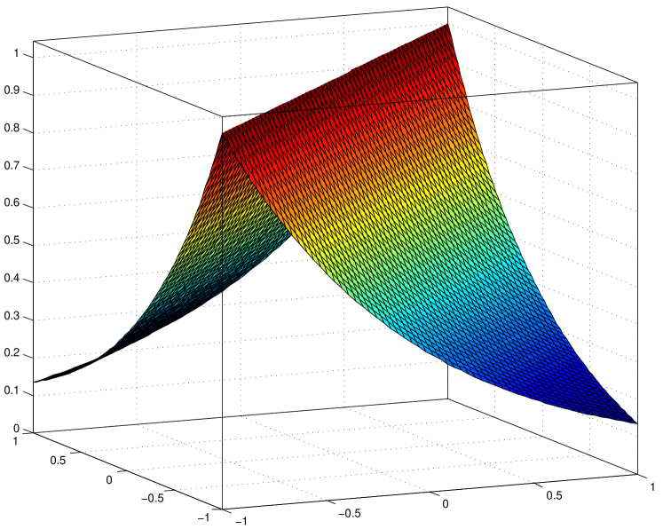
Figure 1: Plot of the function $e^{-|x_{ir}-x_{jr}|}$. Note the boundary $x_{ir}=x_{jr}$ of two adjacent convex polytopes $\mathcal{P}$.

What remains is to show that $\partial\mathcal{F}\subset\mathcal{P}_{0}$. For this, assume that $\partial\mathcal{F}\not\subset\mathcal{P}_{0}$. Then, if the desired set of moments $\{m_{k}^{\star}\}_{k=1}^{s}$ is realizable, there exists another polytope $\mathcal{P}^{\star}\neq\mathcal{P}_{0}$ such that $\partial\mathcal{F}\subset\mathcal{P}^{\star}$. Equivalently, there exists a configuration $x^{\star}\in\mathcal{P}^{\star}$ such that $A(x^{\star})$ has eigenvalues $\{\lambda_{i}(x^{\star})\}_{i=1}^{n}$ with $\sum_{i=1}^{n}\lambda_{i}^{k}(x^{\star})=m_{k}^{\star}$ for all $k=1,\dots,s$. The result follows from the observation that $\mathcal{P}_{0}$ can be obtained from $\mathcal{P}^{\star}$ by changing the relative positions of the robots in $\mathbb{R}^{d}$. Mathematically, this means that there exists a permutation matrix $\Pi\in\mathbb{R}^{nd\times nd}$, i.e., an orthogonal matrix with 0 or 1 entries, such that that if $\mathcal{P}^{\star}=\{x\;|\;Ex\geq 0\}$ with $E\in\mathbb{R}^{n^{2}d\times nd}$, then $\mathcal{P}_{0}=\{x\;|\;E(\Pi x)\geq 0\}$. Therefore, if $x^{\star}\in\mathcal{P}^{\star}$, then $\Pi^{T}x^{\star}\in\mathcal{P}_{0}$. Moreover,

$$A(\Pi^{T}x^{\star})\otimes I_{d}=\Pi(A(x^{\star})\otimes I_{d})\Pi^{T},$$

i.e., a permutation of the robots’ coordinates results in a permutation of the entries of $(A(x)\otimes I_{d})$, where $\otimes$ indicates the Kronecker product between matrices. Since $\Pi$ is orthogonal, $A(\Pi^{T}x^{\star})\otimes I_{d}$ and $A(x^{\star})\otimes I_{d}$ have the same eigenvalues. Therefore, there exists a configuration $\tilde{x}=\Pi^{T}x^{\star}\in\mathcal{P}_{0}$ such that $A(\tilde{x})$ has eigenvalues $\{\lambda_{i}(\tilde{x})\}_{i=1}^{n}$ with $\sum_{i=1}^{n}\lambda_{i}^{k}(\tilde{x})=m_{k}^{\star}$ for all $k=1,\dots,s$. This implies that $\partial\mathcal{F}\subset\mathcal{P}_{0}$.

In the above discussion, we have used the fact that if $\{y_{i}\}_{i=1}^{n}$ are the eigenvalues of $Y\in\mathbb{R}^{n\times n}$ and $\{z_{i}\}_{i=1}^{m}$ are the eigenvalues of $Z\in\mathbb{R}^{m\times m}$, then the eigenvalues of $Y\otimes Z$ are $\{y_{1}z_{1},\dots,y_{1}z_{m},\dots,y_{n}z_{1},\dots,y_{n}z_{m}\}$. This implies that the eigenvalues of $A(x)\otimes I_{d}$ are essentially the eigenvalues of $A(x)$, each one with multiplicity $d$. ∎

Remark 6 (Barrier functions)

The barrier functions $b_{s}(x)$ are necessary in the proof of Theorem 5. If not there, the quantities $m_{k}(x)-m_{k}^{\star}$ are not guaranteed to be positive and, therefore, the potential $f_{s}(x)$ is not necessarily convex in $\mathcal{P}_{0}$. This causes technical difficulties in ensuring a global minimum of $f_{s}(x)$. Also, the analysis in Theorem 5 assumes that $\epsilon_{1},\dots,\epsilon_{s}\to 0$. This essentially restricts the influence of the barrier potential $b_{s}(x)$ to a small neighborhood of the set $\partial\mathcal{F}$, so that the potential $f_{s}(x)$ remains unaffected outside this neighborhood. In practice, the closer the constants $\epsilon_{1},\dots,\epsilon_{s}$ are to zero, the better the approximation of the desired spectral moments. This approximation can be made arbitrarily good.

Remark 7 (Distance metric)

In the preceding analysis, we have employed the $\ell_{1}$ norm ($z=1$) as a distance metric to define the entries of the adjacency matrix (see (3)). This choice is mainly due to technical reasons, since it ensures that $\mathbf{tr}A^{k}(x)$ and, therefore, $f_{s}(x)$, are convex functions. From a practical point of view, the $\ell_{1}$ metric has potential applications in indoor navigation where the presence of obstacles forces the signals to propagate in grid-like environments. Nevertheless, our numerical simulations indicate that the control law herein proposed also performs well for $z=2$ ($\ell_{2}$ norm). We leave a rigorous proof of this case for future work.

IV Numerical Simulations

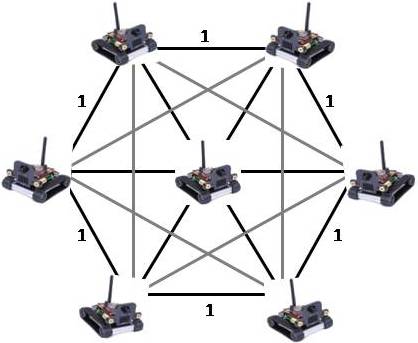
Figure 2: Hexagonal formation of mobile robots.

In this section we present examples of spectral design of mobile robot networks and discuss performance of our proposed approach.

Example 8 (Hexagonal Formation)

Consider the problem of controlling the structure of a network of mobile robots to match the eigenvalue spectrum of the hexagonal network on 7 nodes shown in Fig. 2. The target eigenvalues of the weighted adjacency matrix of this formation are

$$\left\{\lambda_{i}^{\star}\right\}_{i=1}^{7}=\left\{-0.51,\;-0.47,\;-0.40,\;-0.40,\;0.05,\;0.05,\;1.70\right\},$$

and the corresponding spectral moments are

$$\left\{m_{k}^{\star}\right\}_{k=1}^{7}=\left\{0,\;0.53,\;0.64,\;1.22,\;2.02,\;3.47,\;5.90\right\}.$$

The initial configuration of the mobile robot network is that of a random geometric graph on $7$ nodes uniformly distributed in the square $\left[0,1\right]\times\left[0,1\right]$. We applied the proposed control law (15) and studied the evolution of the spectral moments of the network’s adjacency matrix. Fig. 3 shows the evolution of the second, third and fourth moment. As expected, they all converge to the desired values. The asymptotic values of all spectral moments of the network are

$$\left\{m_{k}\right\}_{k=1}^{7}=\left\{0,\;0.53,\;0.65,\;1.23,\;2.04,\;3.50,\;5.95\right\},$$

which are very close to the desired sequence of moments $\left\{m_{k}^{\star}\right\}_{k=1}^{7}$, and slightly on the larger side, as predicted by Theorem 5. The eigenvalues of the weighted adjacency matrix of the final configuration are

$$\left\{\lambda_{i}\right\}_{i=1}^{7}=\left\{-0.52,\;-0.48,\;-0.42,\;-0.40,\;0.02,\;0.10,\;1.70\right\},$$

which are also very close to the desired values. Notice that our approach fits better those eigenvalues further away from the origin, since they are more heavily weighted in the expression of spectral moments, than those close to zero. An alternative approach to overcome this limitation would be to modify our cost function (5) to assign more weight to eigenvalues of small magnitude.

As discussed in Section III-A, we also consider a relaxation of Problem 3, that involves a truncated sequence of the first four moments of the network. In this case, the cost function is given by (12) and the closed loop system is defined in (15), for $s=4$. The asymptotic values of the first four spectral moments of the network are

$$\left\{m_{k}\right\}_{k=1}^{4}=\left\{0,\;0.55,\;0.65,\;1.26\right\}$$

and eigenvalues of the final configuration are

$$\left\{\lambda_{i}\right\}_{i=1}^{7}=\left\{-0.55,\;-0.50,\;-0.42,\;-0.31,\;-0.09,\;0.18,\;1.71\right\},$$

which are remarkably close to the set of desired eigenvalues, especially those far from zero. The main advantages of using a relaxation of Problem 3 are (i) that it reduces the computational cost of the controller, since it only requires the terms $\mathbf{tr}A^{k}$ and $A^{k-1}$, and (ii) that it improves the stability of the numerical behavior of the gradient descent algorithm.

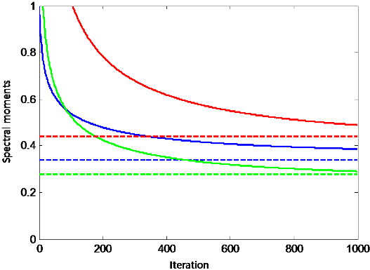
Figure 3: Evolution of second (blue), third (green) and fourth (red) spectral moments towards the moments of the hexagonal formation.

Example 9 (Random Geometric Network)

In this example we consider the problem of matching the eigenvalue spectrum of a particular realization of a random geometric graph on $10$ nodes that are uniformly distributed in $\left[0,1\right]\times\left[0,1\right]$. This target realization is illustrated in Fig. 4, where the thickness of each edge is proportional to its weight. The eigenvalues of the weighted adjacency matrix of this network are

$$\left\{\lambda_{i}^{\star}\right\}_{i=1}^{10} = \left\{-0.89,\;-0.85,\;-0.84,\;-0.79,\;-0.77,\;-0.68,\right.$$

$$\left.-0.61,\;0.02,\;0.27,\;5.16\right\},$$

and the corresponding sequence of spectral moments is

$$\left\{m_{k}^{\star}\right\}_{k>0}=\left\{0,\;3.11,\;13.45,\;71.60,\;368.36,\;1905,\dots\right\}.$$

We applied the control law (15) using the cost function (5) and starting with a different realization of the random geometric graph on $10$ nodes in the square $\left[0,1\right]\times\left[0,1\right]$. In this case, matching the whole set of spectral moments directly provides us with a very good approximation of the eigenvalues spectrum. As before, we also considered the relaxation of Problem 3 involving only a truncated sequence consisting of the first 4 moments. The evolution of the second, third and fourth moments of the network is shown in Fig. 5. The asymptotic values of the spectral moments of the network are

$$\left\{m_{k}\right\}_{k>0}=\left\{0,\;3.13,\;13.46,\;71.63,\dots\right\},$$

which are remarkably close to the desired ones and, as in the previous example, slightly on the larger side. Similarly, the final set of eigenvalues is

$$\left\{\lambda_{i}^{\star}\right\}_{i=1}^{10} = \left\{-0.94,\;-0.87,\;-0.85,\;-0.83,\;-0.74,\;-0.59,\right.$$

$$\left.-0.55,\;-0.27,\;0.50,\;5.16\right\},$$

which is a very good fit to the given eigenvalues, especially for those far from zero.

Figure 4: Random geometric graph with 10 nodes. The width of each edge is proportional to its weight.

V Conclusions and Future Research

In this paper, we proposed a novel control framework to modify the structure of a mobile robot network in order to control the eigenvalue spectrum of its adjacency matrix. We introduced a novel abstraction of the eigenvalue spectrum by means of the spectral moments and derived explicit gradient descent motion controllers for the robots to obtain a network with the desired set of moments. Since the eigenvalue spectrum is uniquely determined by the associated spectral moments, our approach provides a way of controlling the eigenvalues of mobile networks. Convergence to the desired moments was always guaranteed due to convexity of the proposed cost functions. Efficiency of our approach was illustrated in nontrivial computer simulations. The adjacency matrix eigenvalue spectrum is relevant to the performance of many distributed coordination algorithms run over a network. Therefore, our approach is particularly useful in providing network structures that are optimal with respect to networked coordination objectives.

Future work involves theoretical guarantees for the Euclidean distance metric ($z=2$ in (3)), as well as extension of our results to the spectrum of Laplacian matrix of the network. Moreover, the relaxation of Problem 3 to a truncated sequence of moments does not guarantee (mathematically) a good fit of the complete distribution of eigenvalues. Therefore, a natural question is to characterize the set of graphs most of whose spectral information is contained in a relatively small set of low-order moments.

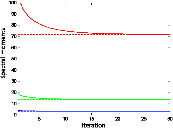
Figure 5: Evolution of second (blue), third (green) and fourth (red) spectral moments towards the moments of the random geometric graph.

References

- [1] K. M. Lynch and M. T. Mason, “Stable pushing: Mechanics, controllability and planning,” International Journal of Robotics Research, vol. 15, pp. 533-556, 1996.
- [2] M. J. Mataric, M. Nilsson, and K. Simsarian, “Cooperative multi-robot box-pushing,” IEEE/RSJ International Conference on Intelligent Robots and Systems, pp. 556-561, 1995.
- [3] Z. Wang and V. Kumar, “Object closure and manipulation by multiple cooperating mobile robots,” International Symposium on Distributed Autonomous Robotic Systems, pp. 394-399, 2002.
- [4] J. Cortes, S. Martinez, T. Karatas, and F. Bullo, “Coverage control for mobile sensing networks,” IEEE Transactions on Robotics and Automation, vol. 20, pp. 243-255, 2004.
- [5] L. E. Parker, “Distributed algorithms for multi-robot observation of multiple moving targets,” Autonomous Robots, vol. 12, pp. 231-255, 2002.
- [6] S. Poduri and G. S. Sukhatme, “Constrained coverage for mobile sensor networks,” IEEE International Conference on Robotics and Automation, pp. 165-172, 2004.
- [7] A. Jadbabaie, J. Lin, and A. S. Morse, “Coordination of groups of mobile autonomous robots using nearest neighbor rules,” IEEE Transactions on Automatic Control, vol. 48, pp. 988-1001, 2003.
- [8] R. Olfati-Saber, J. A. Fax, and R. M. Murray, “Consensus and cooperation in networked multi-robot systems,” Proceedings of the IEEE, vol. 95, pp. 215-33, 2007.
- [9] W. Ren and R. Beard, “Consensus seeking in multi-robot systems under dynamically changing interaction topologies,” IEEE Transactions on Automatic Control, vol. 50, pp. 655-661, 2005.
- [10] J. P. Desai, J. P. Ostrowski, and V. Kumar, “Modeling and control of formations of nonholonomic mobile robots,” IEEE Transactions on Robotics and Automation, vol. 17, pp. 905-908, 2001.
- [11] J. Lawton, B. Young, and R. Beard, “A decentralized approach to elementary formation maneuvers,” IEEE International Conference on Robotics and Automation, pp. 2728-2733, 2005.
- [12] M. Mesbahi and F. Y. Hadaegh, “Formation flying control of multiple spacecraft via graphs, matrix inequalities and switching,” AIAA Journal of Guidance, Control and Dynamics, vol. 24, pp. 369-377, 2001.
- [13] R. Olfati-Saber, “Flocking for multi-robot dynamic systems: Algorithms and theory,” IEEE Transactions on Automatic Control, vol. 51, pp. 401-420, 2006.
- [14] H. G. Tanner, A. Jadbabaie, and G. J. Pappas, “Flocking in fixed and switching networks,” IEEE Transactions on Automatic Control, vol. 52, pp. 863-868, 2007.
- [15] S. L. Smith and F. Bullo, “Target assignment for robotic networks: Asymptotic performance under limited communication,” American Control Conference, pp. 1155-1160, 2007.
- [16] M. M. Zavlanos and G. J. Pappas, “Dynamic assignment in distributed motion planning with local coordination,” IEEE Transactions on Robotics, vol. 24, pp. 232-242, 2008.
- [17] S. Kloder and S. Hutchinson, “Path planning for permutation-invariant multi-robot formations,” IEEE Transactions on Robotics, vol. 22, pp. 650-665, 2006.
- [18] V.M. Preciado, Spectral Analysis for Stochastic Models of Large-Scale Complex Dynamical Networks, Ph.D. dissertation, Dept. Elect. Eng. Comput. Sci., MIT, Cambridge, MA, 2008.
- [19] D.J. Aldous, “Some Inequalities for Reversible Markov Chains,” J. London Math. Soc., vol. 25, pp. 564-576, 1982.
- [20] L.M. Pecora and T.L. Carroll, “Master Stability Functions for Synchronized Coupled Systems,” Physics Review Letters, vol. 80, pp. 2109-2112, 1998.
- [21] V.M. Preciado, and G.C. Verghese, “Synchronization in Generalized Erdös-Rényi Networks of Nonlinear Oscillators,” IEEE Conference on Decision and Control, pp. 4628-4633, 2005.
- [22] M. Draief, A. Ganesh, and L. Massoulié, “Thresholds for Virus Spread on Networks,” Annals of Applied Probability, vol. 18, pp. 359-378, 2008.
- [23] V.M. Preciado, and A. Jadbabaie, “Spectral Analysis of Virus Spreading in Random Geometric Networks,” IEEE Conference on Decision and Control , 2009.
- [24] N.A. Lynch, Distributed Algorithms, Morgan Kaufmann Publishers, 1997.
- [25] A. Fax, and R. M. Murray, “Information Flow and Cooperative Control of Vehicle Formations,” IEEE Transactions on Automatic Control, vol. 49, pp. 1465-1476, 2004.
- [26] R. Olfati-Saber, and R. M. Murray, “Consensus Problems in Networks of robots with Switching Topology and Time-Delays,” IEEE Transactions on Automatic Control, vol. 49, pp. 1520-1533, 2004.
- [27] A. Ghosh, and S. Boyd, “Growing Well-Connected Graphs,” Proc. of the 45th IEEE Conference on Decision and Control, pp. 6605-6611, 2006.
- [28] R. Grone, R. Merris, and V.S. Sunder, “The Laplacian Spectrum of a Graph,” SIAM Journal Matrix Analysis and Applications, vol. 11, pp. 218-238, 1990.
- [29] Y. Kim, and M. Mesbahi, “On Maximizing the Second-Smallest Eigenvalue of a State Dependent Graph Laplacian,” IEEE Transactions on Automatic Control, vol. 51, pp. 116-120, 2006.
- [30] M.C. DeGennaro, and A. Jadbabaie, “Decentralized Control of Connectivity for Multi-robot Systems,” IEEE Conference on Decision and Control, pp. 3628-3633, 2006.
- [31] V. M. Preciado, M. M. Zavlanos, A. Jadbabaie and G. J. Pappas, “Distributed control of the Laplacian spectral moments of a network,” American Control Conference, pp. 4462-4467, 2010.