An Operator–like Description of Love Affairs

Abstract

We adopt the so–called occupation number representation, originally used in quantum mechanics and recently considered in the description of stock markets, in the analysis of the dynamics of love relations. We start with a simple model, involving two actors (Alice and Bob): in the linear case we obtain periodic dynamics, whereas in the nonlinear regime either periodic or quasiperiodic solutions are found. Then we extend the model to a love triangle involving Alice, Bob and a third actress, Carla. Interesting features appear, and in particular we find analytical conditions for the linear model of love triangle to have periodic or quasiperiodic solutions. Numerical solutions are exhibited in the nonlinear case.

1 Introduction and preliminaries

In a series of recent papers one of us (F.B.) used the framework of quantum mechanics, operator algebra and, in particular, of the so–called occupation number representation to discuss some toy models of stock markets [1, 2, 3, 4]. The main motivation for such an approach was that during the time evolution the main variables of a closed stock market can take only discrete values. This feature is well described by using the eigenvalues of some operators which describe these variables, the so-called observables of the market. Moreover, the closed stock markets we have considered admit conserved quantities, like the total number of shares or the total amount of cash, and these conserved quantities are well described in our framework. Here we want to show how the same general approach could be used in dealing with a completely different problem, i.e., the analysis of a love affair. In fact, it is natural to measure the mutual affection of the actors of our model using natural numbers (the higher the number, the stronger the love), and to think that some conserved quantities do exist in the game. It might be worth recalling that sophisticated mathematical tools have been used several times in the analysis of this problem, producing many interesting results which can be found in [5, 6, 7, 8, 9, 10], as well as in an extensive monograph, [11]. For instance, in [9], some simple dynamical models involving coupled ordinary differential equations and describing the time variation of the love or hate in a romantic relationship are considered. In particular, a linear model for two individuals is discussed, and the extension to a love triangle, with nonlinearities causing chaotic dynamics, is also taken into account.

It should also be considered that in the last few years a growing interest in classical application of quantum ideas has appeared in the literature. This involves very different fields like economics, [12, 13], biology, [14], and sociology, [15, 16] and references therein, just to cite a few, and is a strong encouragement to carry on our analysis.

The paper is organized as follows. In Section 2, we consider a first simple model involving two lovers, Alice and Bob, and we analyze the dynamics of their relationship starting from very natural technical assumptions. Both a linear and a nonlinear model are considered; then, the equations of motion are solved analytically (for the linear model) and numerically (for the nonlinear model), under suitable (and fairly good) approximations.

In Section 3, we consider a model in which Bob has two relationships at the same time, and again we carry on our dynamical analysis. Also in this case we find an explicit solution for the linear model, while the nonlinear one is discussed numerically. Section 4 contains our conclusions, while, to keep the paper self–contained, the Appendix reviews few useful facts in quantum mechanics and occupation number representation.

2 A first model

The first model we have in mind consists of a couple of lovers, Bob and Alice, which mutually interact exhibiting a certain interest for each other. Of course, there are several degrees of possible interest, and to a given Bob’s interest for Alice (LoA, level of attraction) there corresponds a related reaction (i.e., a different LoA) of Alice for Bob. Now, let us see how this mechanism could be described in terms of creation and annihilation operators.

Extending what has been done in [1, 2, 3, 4], we now introduce $a_{1}$ and $a_{2}$, two independent bosonic operators. This means that they obey the commutation rules

$$[a_{i},a^{\dagger}_{k}]=a_{i}\,a^{\dagger}_{k}-a^{\dagger}_{k}\,a_{i}=1\!\!1\,\delta_{i,k},$$ (2.1)

while all the other commutators are trivial: $[a_{i},a_{k}]=[a^{\dagger}_{i},a^{\dagger}_{k}]=0$, for all $i$ and $k$. Further, let $\varphi_{0}^{(j)}$ be the vacuum of $a_{j}$, $a_{j}\,\varphi_{0}^{(j)}=0$, $j=1,2$. By using $\varphi_{0}^{(j)}$ and the operators $a_{j}^{\dagger}$, we may construct the following vectors:

$$\varphi_{n_{j}}^{(j)}:=\frac{1}{\sqrt{n_{j}!}}\,(a_{j}^{\dagger})^{n_{j}}\,\varphi_{0}^{(j)},\qquad\varphi_{n_{1},n_{2}}:=\varphi_{n_{1}}^{(1)}\otimes\varphi_{n_{2}}^{(2)},$$ (2.2)

where $n_{j}=0,1,2,\ldots$, and $j=1,2$. Let us also define $N_{j}=a_{j}^{\dagger}\,a_{j}$, $j=1,2$, and $N=N_{1}+N_{2}$. Hence (see the Appendix), for all $j$,

$$\left\{\begin{array}[]{ll}N_{j}\varphi_{n_{1},n_{2}}=n_{j}\varphi_{n_{1},n_{2}},\\ N_{j}\,a_{j}\,\varphi_{n_{1},n_{2}}=(n_{j}-1)\,a_{j}\varphi_{n_{1},n_{2}},\\ N_{j}\,a_{j}^{\dagger}\,\varphi_{n_{1},n_{2}}=(n_{j}+1)\,a_{j}^{\dagger}\varphi_{n_{1},n_{2}}.\end{array}\right.$$

Then, we also have $N\varphi_{n_{1},n_{2}}=(n_{1}+n_{2})\varphi_{n_{1},n_{2}}$. As usual, the Hilbert space $\mathcal{H}$ in which the operators live is obtained by taking the closure of the linear span of all these vectors, for $n_{j}\geq 0$, $j=1,2$. A state over the system is a normalized linear functional $\omega_{n_{1},n_{2}}$ labeled by two quantum numbers $n_{1}$ and $n_{2}$ such that $\omega_{n_{1},n_{2}}(x)=\left<\varphi_{n_{1},n_{2}},x\,\varphi_{n_{1},n_{2}}\right>$, where $\left<.,.\right>$ is the scalar product in $\mathcal{H}$ and $x$ is an arbitrary operator on $\mathcal{H}$.

In this paper we associate the (integer) eigenvalue $n_{1}$ of $N_{1}$ to the LoA that Bob experiences for Alice: the higher the value of $n_{1}$ the more Bob desires Alice. For instance, if $n_{1}=0$, Bob just does not care about Alice. We use $n_{2}$, the eigenvalue of $N_{2}$, to label the attraction of Alice for Bob. A well known (surely simplified) law of attraction stated in our language says that if $n_{1}$ increases then $n_{2}$ decreases and viceversa. Following the same general strategy as in [1, 2, 3, 4], this suggests to use the following self–adjoint operator to describe the dynamics (see Appendix) of the relationship:

$$H=\lambda\left(a_{1}^{M_{1}}\,{a_{2}^{\dagger}}^{M_{2}}+\hbox{h.c.}\right).$$ (2.4)

Here, h.c. stands for hermitian conjugate, and $M_{1}$ and $M_{2}$ give a measure of the kind of mutual reaction between Bob and Alice: if $M_{1}$ is large compared to $M_{2}$, Bob will change his status very fast compared with Alice. The opposite change is expected for $M_{2}$ much larger than $M_{1}$, while, for $M_{1}$ close to $M_{2}$, they will react essentially with the same speed. These claims will be justified in the rest of the paper. However, as it is already clear at this stage, it is enough to introduce a single index $M$ rather than $M_{1}$ and $M_{2}$, since $M$ plays the role of a relative behavior. For this reason we will choose the hamiltonian

$$H=\lambda\left(a_{1}^{M}{a_{2}^{\dagger}}+\hbox{h.c.}\right),$$ (2.5)

where $\lambda$ is the interaction parameter (which could also be seen as a time scaling parameter). The physical meaning of $H$ can be deduced considering the action of, say, $a_{1}^{M}\,{a_{2}^{\dagger}}$ on the vector describing the system at time $t=0$, $\varphi_{n_{1},n_{2}}$. This means that, at $t=0$, Bob is in the state $n_{1}$, i.e. $n_{1}$ is Bob’s LoA, while Alice is in the state $n_{2}$. However, because of the definition of $\varphi_{n_{1},n_{2}}$, $a_{1}^{M}\,{a_{2}^{\dagger}}\,\varphi_{n_{1},n_{2}}$, which is different from zero only if $M<n_{1}$, is proportional to $\varphi_{n_{1}-M,n_{2}+1}$. Hence, Bob’s interest for Alice decreases of $M$ units while Alice’s interest for Bob increases of 1 unit. Of course, the Hamiltonian (2.5) also contains the opposite behavior. Indeed, because of the presence of $a_{2}\,{a_{1}^{\dagger}}^{M}$ in $H$, if $n_{2}\geq 1$ we see that $a_{2}\,{a_{1}^{\dagger}}^{M}\varphi_{n_{1},n_{2}}$ is proportional to $\varphi_{n_{1}+M,n_{2}-1}$: hence, Bob’s interest is increasing (of $M$ units) while Alice looses interest in Bob. It is not hard to check that $I(t):=N_{1}(t)+M\,N_{2}(t)$ is a constant of motion: $I(t)=I(0)=N_{1}(0)+M\,N_{2}(0)$, for all $t\in\mathbb{R}$. This is a consequence of the following commutation result: $[H,I]=0$. Therefore, during the time evolution, a certain global attraction is preserved and can only be exchanged between Alice and Bob: notice that this reproduces our original point of view on the love relation between Alice and Bob.

Now we have all the ingredients to derive the equations of motion for our model. These are found by assuming, as we have already done implicitly, the same Heisenberg–like dynamics which works perfectly for quantum systems, and which is natural in the present operatorial settings. Of course, this is a strong assumption and should be checked a posteriori, finding the dynamical behavior deduced in this way and showing that this gives reasonable results. More explicitly, we are assuming that the time evolution $X(t)$ of a given observable $X$ of the system is given by $X(t)=e^{iHt}Xe^{-iHt}$. The equations of motion for the number operators $N_{1}(t)$ and $N_{2}(t)$, which are needed to deduce the rules of the attraction, turn out to be the following:

$$\left\{\begin{array}[]{ll}\dot{N}_{1}(t)=i\,\lambda M\left(a_{2}^{\dagger}(t)(a_{1}(t))^{M}-a_{2}(t)(a_{1}(t)^{\dagger})^{M}\right),\\ \dot{N}_{2}(t)=-i\,\lambda\left(a_{2}^{\dagger}(t)(a_{1}(t))^{M}-a_{2}(t)(a_{1}(t)^{\dagger})^{M}\right).\end{array}\right.$$ (2.8)

By using this system, it is straightforward to check directly that $I(t)$ does not depend on time. However, this system is not closed, so that it may be more convenient to replace (2.8) by the differential system for the annihilation operators $a_{1}(t)$ and $a_{2}(t)$:

$$\left\{\begin{array}[]{ll}\dot{a}_{1}(t)=-i\,\lambda M\,a_{2}(t)(a_{1}(t)^{\dagger})^{M-1}\\ \dot{a}_{2}(t)=-i\,\lambda\,(a_{1}(t))^{M}.\end{array}\right.$$ (2.11)

Then, we may use the solutions of this system to construct $N_{j}(t)=a_{j}^{\dagger}(t)\,a_{j}(t)$, $j=1,2$. Equations (2.11), together with their adjoint, produce a closed system. Of course, there exists a simple situation for which the system (2.11) can be exactly solved quite easily: $M=1$. In this case, which corresponds to the assumption that Alice and Bob react with the same speed, system (2.11) is already closed and the solution is easily found:

$$a_{1}(t)=a_{1}\cos(\lambda t)-ia_{2}\sin(\lambda t),\qquad a_{2}(t)=a_{2}\cos(\lambda t)-ia_{1}\sin(\lambda t).$$ (2.12)

Now, if we assume that at $t=0$ Bob and Alice are respectively in the $n_{1}$’th and $n_{2}$’th LoA’s, the state of the system at $t=0$ is $\omega_{n_{1},n_{2}}$ (see Appendix). Therefore, calling $n_{j}(t):=\omega_{n_{1},n_{2}}(N_{j}(t))$, $j=1,2$, we find that

$$n_{1}(t)=n_{1}\cos^{2}(\lambda t)+n_{2}\sin^{2}(\lambda t),\qquad n_{2}(t)=n_{2}\cos^{2}(\lambda t)+n_{1}\sin^{2}(\lambda t),$$ (2.13)

so that, in particular, $\omega_{n_{1},n_{2}}(I(t))=n_{1}+n_{2}$, as expected. The conclusion is quite simple and close to our view of how the law of the attraction works: the infatuations of Alice and Bob oscillate in such a way that when Bob’s LoA increases, that of Alice decreases and viceversa, with a period which is directly related to the value of the interaction parameter $\lambda$. In particular, as is natural, setting $\lambda=0$ in equation (2.13), implies that both Alice and Bob stay in their initial LoA’s. The solution in (2.13) justifies, in a sense, our approach: the law of the attraction between Alice and Bob is all contained in a single operator, the hamiltonian of the model, whose explicit expression can be easily deduced using rather general arguments. The related dynamics is exactly the one we expected to find. Hence, the use of the Heisenberg equations of motion seems to be justified, at least for this simple model. A similar result was found for the linear model also in [9], under suitable assumptions about the parameters.

Much harder is the situation when $M>1$. In this case we do need to consider the adjoint of (2.11) to close the system and, nevertheless, an exact solution can not be obtained. However, it is possible to generate a numerical scheme to find solutions of our problem, and this is the content of the next subsection.

2.1 Numerical results for $M>1$

The first remark is that, as stated above, the Hilbert space of our theory, $\mathcal{H}$, is infinite–dimensional. This means that both Bob and Alice may experience infinite different LoA’s. This makes the situation rather hard from a computational point of view and, furthermore, looks like a useless difficulty. As a matter of fact, it is enough to assume that Bob (respectively, Alice) may pass through $L_{1}$ (respectively, $L_{2}$) different LoA’s ($L_{1}$ and $L_{2}$ fixed positive integers), which efficiently describe their mutual attraction. This means that our effective Hilbert space, $\mathcal{H}_{eff}$, is finite–dimensional and is generated by the orthonormal basis

$$\mathcal{F}=\{\varphi_{\underline{n}}:=\varphi_{n_{1},n_{2}},\quad n_{j}=0,1,\ldots,L_{j},\,j=1,2\}=\{\varphi_{\underline{n}},\quad\underline{n}\in\mathcal{K}\},$$ (2.14)

with obvious notation. Hence, $dim(\mathcal{H}_{eff})=(L_{1}+1)(L_{2}+1)$ is exactly the cardinality of $\mathcal{K}$.

Calling $1\!\!1_{eff}$ the identity operator over $\mathcal{H}_{eff}$ the closure relation for $\mathcal{F}$ looks like $\sum_{\underline{n}\in K}|\varphi_{\underline{n}}><\varphi_{\underline{n}}|=1\!\!1_{eff}$. It is a standard exercise in quantum mechanics to check that

$$\left\{\begin{array}[]{ll}(a_{1})_{\underline{k},\underline{k}^{\prime}}:=<\varphi_{\underline{k}},a_{1}\varphi_{\underline{k}^{\prime}}>=\sqrt{k_{1}^{\prime}}\,\delta_{k_{1},k_{1}^{\prime}-1}\,\delta_{k_{2},k_{2}^{\prime}},\\ (a_{2})_{\underline{k},\underline{k}^{\prime}}:=<\varphi_{\underline{k}},a_{2}\varphi_{\underline{k}^{\prime}}>=\sqrt{k_{2}^{\prime}}\,\delta_{k_{2},k_{2}^{\prime}-1}\,\delta_{k_{1},k_{1}^{\prime}},\end{array}\right.$$ (2.17)

so that, by using the resolution of the identity in $\mathcal{H}_{eff}$, we can produce a projected expression of the operators $a_{j}$ as follows:

$$a_{1}\rightarrow A_{1}:=\sum_{\underline{k},\underline{k}^{\prime}\in K}\,<\varphi_{\underline{k}},a_{1}\varphi_{\underline{k}^{\prime}}>|\varphi_{\underline{k}}><\varphi_{\underline{k}^{\prime}}|=\sum_{\underline{k}^{\prime}\in K}\,\sqrt{k_{1}^{\prime}}\,|\varphi_{k_{1}^{\prime}-1,k_{2}^{\prime}}><\varphi_{k_{1}^{\prime}k_{2}^{\prime}}|,$$ (2.18)

$$a_{2}\rightarrow A_{2}:=\sum_{\underline{k},\underline{k}^{\prime}\in K}\,<\varphi_{\underline{k}},a_{2}\varphi_{\underline{k}^{\prime}}>|\varphi_{\underline{k}}><\varphi_{\underline{k}^{\prime}}|=\sum_{\underline{k}^{\prime}\in K}\,\sqrt{k_{2}^{\prime}}\,|\varphi_{k_{1}^{\prime},k_{2}^{\prime}-1}><\varphi_{k_{1}^{\prime}k_{2}^{\prime}}|.$$

In other words, while the $a_{j}$’s act on $\mathcal{H}$, the related matrices $A_{j}$’s act on the finite dimensional Hilbert space $\mathcal{H}_{eff}$. This means that, while the $a_{j}(t)$’s are unbounded operators (which could be represented as infinite matrices), the $A_{j}(t)$’s are $(L_{1}+1)(L_{2}+1)\times(L_{1}+1)(L_{2}+1)$ matrices whose elements, for $t=0$, can be deduced by (2.18). Thus, these are really bounded operators and, as we will see, they all have the following property: for all choices of $L_{j}$ a certain power $R_{j}$ exists such that $A_{j}^{R_{j}}=0$, $(A_{j}^{\dagger})^{R_{j}}=0$, condition which is not shared by the original $a_{j}$. This fact is related to the approximation which produces $\mathcal{H}_{eff}$ out of the original $\mathcal{H}$. Now, system (2.11) can be written in a formally identical way as

$$\left\{\begin{array}[]{ll}\dot{A}_{1}(t)=-i\,\lambda M\,A_{2}(t)(A_{1}(t)^{\dagger})^{M-1},\\ \dot{A}_{2}(t)=-i\,\lambda\,(A_{1}(t))^{M},\end{array}\right.$$ (2.21)

where $A_{1}(t)$ and $A_{2}(t)$ are bounded matrices rather than unbounded operators. It should be stressed that the change $a_{j}\rightarrow A_{j}$ does not destroy the existence of an integral of motion, which is clearly $I_{eff}(t)=\mathcal{N}_{1}(t)+M\mathcal{N}_{2}(t)$, where $\mathcal{N}_{j}(t)=A_{j}(t)^{\dagger}A_{j}(t)$.

The numerical scheme is quite simple: we just have to fix the dimensionality of $\mathcal{H}_{eff}$, that is $L_{1}$ and $L_{2}$ (i.e., the number of LoA’s), the value of $M$ in (2.5), and the matrices $A_{j}(0)$. Then, by choosing a reliable scheme for integrating numerically a set of ordinary differential equations, we may construct a solution for the equations (2.21) in a prescribed time interval. Fron now on, we take $L_{1}=L_{2}=K$ ($K$ suitable positive integer), whereupon $dim(\mathcal{H}_{eff})=(K+1)^{2}$, and we consider the orthonormal basis of $\mathcal{H}_{eff}$ in the following order (the order is important to fix the form of the matrix!):

$$\mathcal{F}=\left\{\varphi_{00},\varphi_{01},\ldots,\varphi_{0K},\varphi_{10},\varphi_{11},\ldots,\varphi_{1K},\ldots,\varphi_{K0},\varphi_{K1},\ldots,\varphi_{KK}\right\}.$$

Then we get

$$A_{1}(0) =\left(\begin{array}[]{cccccc}\mathbf{0}_{K}&\mathbf{0}_{K}&\ldots&\ldots&\mathbf{0}_{K}&\mathbf{0}_{K}\\ 1\!\!1_{K}&\mathbf{0}_{K}&\ldots&\ldots&\mathbf{0}_{K}&\mathbf{0}_{K}\\ \mathbf{0}_{K}&\sqrt{2}1\!\!1_{K}&\mathbf{0}_{K}&\ldots&\mathbf{0}_{K}&\mathbf{0}_{K}\\ \mathbf{0}_{K}&\mathbf{0}_{K}&\sqrt{3}1\!\!1_{K}&\ldots&\mathbf{0}_{K}&\mathbf{0}_{K}\\ \ldots&\ldots&\ldots&\ldots&\ldots&\ldots\\ \ldots&\ldots&\ldots&\ldots&\ldots&\ldots\\ \mathbf{0}_{K}&\mathbf{0}_{K}&\ldots&\ldots&\sqrt{K-1}1\!\!1_{K}&\mathbf{0}_{K}\end{array}\right),$$

$$A_{2}(0) =\left(\begin{array}[]{ccccc}\underline{x}&\mathbf{0}_{K}&\ldots&\ldots&\mathbf{0}_{K}\\ \mathbf{0}_{K}&\underline{x}&\ldots&\ldots&\mathbf{0}_{K}\\ \ldots&\ldots&\ldots&\ldots&\ldots\\ \ldots&\ldots&\ldots&\ldots&\ldots\\ \mathbf{0}_{K}&\mathbf{0}_{K}&\ldots&\ldots&\underline{x}\\ \end{array}\right),$$

where $\mathbf{0}_{K}$ and $1\!\!1_{K}$ are the null and the identity matrices of order $K$ respectively, whereas

$$\underline{x}=\left(\begin{array}[]{ccccc}0&0&0&\ldots&0\\ 1&0&0&\ldots&0\\ 0&\sqrt{2}&0\ldots&0\\ \ldots&\ldots&\ldots&\ldots&\ldots\\ 0&0&\ldots&\sqrt{K-1}&0\end{array}\right).$$

It is easy to verify that $A_{1}(0)^{K-1}\neq\mathbf{0}_{K}$ and $A_{2}(0)^{K-1}\neq\mathbf{0}_{K}$, while $A_{1}(0)^{K}=A_{2}(0)^{K}=\mathbf{0}_{K}$. This simply means that, since because of our original approximation $\mathcal{H}\rightarrow\mathcal{H}_{eff}$, there are only $K+1$ different levels; then, if we try to act more than $K+1$ times on a certain state, the only effect we get is just to annihilate that state. In other words, we can not move Bob or Alice to a $-1$ or $K+1$ LoA by acting with $A_{j}$ or $A_{j}^{\dagger}$ since these states do not exist! However, this argument does not apply to the operators $a_{j}$ in $\mathcal{H}$, since in the original Hilbert space there is no upper bound to the value of the LoA’s of the two lovers.

Suppose now that for $t=0$ the system is in the state $\omega_{\underline{n}}$, where $\underline{n}=(n_{1},n_{2})$. This means, as usual, that $\underline{n}$ describes the LoA of Alice and Bob. As we have done explicitly for $M=1$, if we want to know how Bob’s LoA varies with time, we have to compute

$$n_{1}(t):=<\varphi_{\underline{n}},\mathcal{N}_{1}(t)\varphi_{\underline{n}}>=\|A_{1}(t)\varphi_{\underline{n}}\|^{2}=\sum_{\underline{k}\in K}|(A_{1}(t))_{\underline{k},\underline{n}}(t)|^{2},$$

in terms of the matrix elements. Analogously, to compute how Alice’s LoA varies with time, we need to compute

$$n_{2}(t):=<\varphi_{\underline{n}},\mathcal{N}_{2}(t)\varphi_{\underline{n}}>=\|A_{2}(t)\varphi_{\underline{n}}\|^{2}=\sum_{\underline{k}\in K}|(A_{2}(t))_{\underline{k},\underline{n}}(t)|^{2}.$$

The system (2.21) is numerically integrated for different choices of $K$ by taking $M=2$ and $\lambda=0.1$. We use a variable order Adams–Bashforth–Moulton PECE solver [20] as implemented in MATLAB^®’s ode113 routine.

Figure 1: $K=3$, $M=2$: Alice’s and Bob’s LoA’s vs. time with initial condition $(1,1)$. A periodic behavior is observed.

In Figure 1, the time evolutions of Alice’s and Bob’s LoA’s in the case $K=3$ with equal initial conditions $n_{1}(0)=n_{2}(0)=1$ are displayed. Two clear oscillations in opposite phase can be observed: Alice and Bob react simultaneously but in different directions. This is in agreement with our naive point of view of Alice–Bob’s love relationship, and confirms that the Heisenberg equations of motion can really be used to describe the dynamics of this classical system, also in this nonlinear (and likely more realistic) case. The horizontal dotted line on the top in Figure 1 (and also in Figures 2 and 3 below) represents the integral of motion $I_{eff}(t)$; in some sense, it provides a check of the quality of the numerical solution.

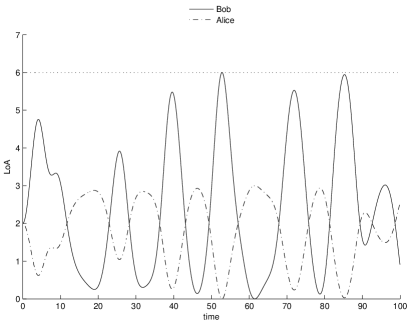
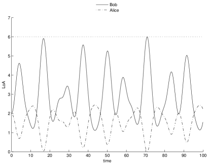
Figure 2: Alice’s and Bob’s LoA’s vs. time with initial conditions $(2,2)$ and $M=2$: $K=3$ (top left), $K=6$ (top right), $K=7$ (bottom left), $K=8$ (bottom right): $K=6$ is already a good approximation.

In Figure 2, the evolution of Alice’s and Bob’s LoA’s with initial conditions $(2,2)$ for different dimensions of $\mathcal{H}_{eff}$ is plotted. As it can be observed, when $K=3$, the values of LoA’s go beyond the maximum admissible value ($K$); this suggests to improve the approximation, i.e. to increase the dimension of $\mathcal{H}_{eff}$. By taking $K=6$, we find that Alice’s and Bob’s LoA’s assume values within the bounds. Moreover, by performing the numerical integration with higher values of $K$ ($K=7$ and $K=8$), the same dynamics as when $K=6$ is recovered. We also see that, as in Figure 1, $n_{1}(t)$ increases when $n_{2}(t)$ decreases, and viceversa.

The same main features are found in Figure 3, where the initial condition $(1,3)$ and different values of $K$ ($K=5,6,7,8$) are considered. The choice $K=5$ turns out to be a poor approximation; in fact, the values of LoA’s can not be described in its $\mathcal{H}_{eff}$. On the contrary, already for $K=6$, the related $\mathcal{H}_{eff}$ turns out to be a fairly good substitute of $\mathcal{H}$, since the values of LoA’s do not exceed the limits during the time evolution. Furthermore, the dynamics is stable for increasing values of $K$.

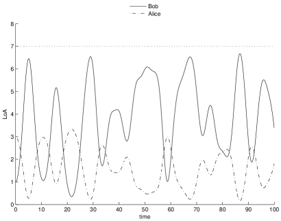
Figure 3: Alice’s and Bob’s LoA’s vs. time with initial condition $(1,3)$ and $M=2$: $K=5$ (top left), $K=6$ (top right), $K=7$ (bottom left), $K=8$ (bottom right): again, $K=6$ is already a good approximation.

Let us summarize the situation: as a consequence of our approximation, $\mathcal{H}\rightarrow\mathcal{H}_{eff}$, we need to replace $I(t)$ with $I_{eff}(t)=\mathcal{N}_{1}(t)+M\,\mathcal{N}_{2}(t)$. As already noticed, because of (2.21), $\dot{I}_{eff}(t)=0$, i.e., $I_{eff}(t)$ is a constant of motion for the approximate model. Hence, it happens that if $\mathcal{N}_{2}(t)$ decreases during its time evolution, $\mathcal{N}_{1}(t)$ must increase since $I_{eff}(t)$ has to stay constant. In this way, for some value of $t$, it may happen that $\mathcal{N}_{1}(t)>K$ (see Figure 2 for $K=3$, and Figure 3 for $K=5$). This problem is cured simply by fixing higher values of $K$, as numerically shown in Figures 2 and 3, where the choice $K=6$ allows us to capture the right dynamics, that remains unchanged also when $K=7$ and $K=8$. In a sense, the dimension of $\mathcal{H}_{eff}$ can be a priori fixed looking at the value of the integral of motion. In fact, if for some $\overline{t}$, $\mathcal{N}_{2}(\overline{t})=0$, then $\mathcal{N}_{1}(\overline{t})$ is equal to $I_{eff}(0)$, which in turn depends on the initial conditions. Therefore, the dimension of $\mathcal{H}_{eff}$ must be greater than or equal to $I_{eff}(0)$; last, but not least, our numerical tests allow us to conjecture that, increasing the dimension of $\mathcal{H}_{eff}$, the resulting dynamics is not affected.

It may be worth stressing that this feature only appears because of the numerical approach we are adopting here, and nothing has to do with our general framework. This is clear, for instance, considering the solution of the linear situation where no approximation is needed and no effect like this is observed.

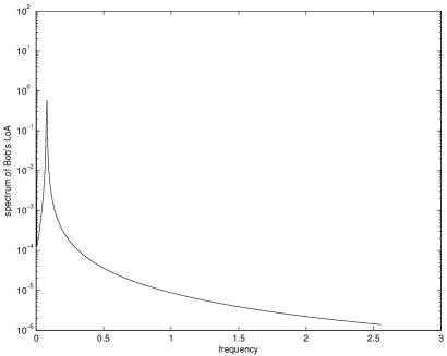
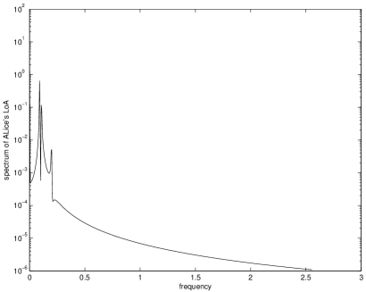
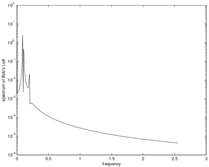
Figure 4: Power spectra vs. frequency of numerical solutions for Alice’s LoA (left) and Bob’s LoA (right) for initial conditions $(1,1)$ (top: periodic dynamics) and $(1,3)$ (bottom: quasiperiodic dynamics).

In this nonlinear case, the numerical results seem to show that a periodic motion is not recovered for all initial conditions, contrarily to what analytically proved in the case $M=1$. In Figures 2 and 3, rather than a simple periodic time evolution (like that displayed in Figure 1), a quasiperiodic behavior seems to emerge, as the plots of the power spectra of the time series representing the numerical solutions (see Figure 4, bottom) also suggest. However, what emerges from our numerical tests is that, once the dimension of $\mathcal{H}_{eff}$ is sufficient to capture the dynamics, only periodic or quasiperiodic solutions are obtained. This does not exclude that, for initial conditions requiring dimensions of the Hilbert space higher than those considered here, a richer dynamics (say, chaotic) may arise. Further numerical investigations in this direction are in progress.

3 A generalization: a love triangle

In this section we will generalize our previous model by inserting a third ingredient. Just to fix the ideas, we will assume that this third ingredient, Carla, is Bob’s lover, and we will use the same technique to describe the interactions among the three. The situation can be summarized as follows:

1. Bob can interact with both Alice and Carla, but Alice (respectively, Carla) does not suspect of Carla’s (respectively, Alice’s) role in Bob’s life;

2. if Bob’s LoA for Alice increases then Alice’s LoA for Bob decreases and viceversa;

3. analogously, if Bob’s LoA for Carla increases then Carla’s LoA for Bob decreases and viceversa;

4. if Bob’s LoA for Alice increases then his LoA for Carla decreases (not necessarily by the same amount) and viceversa.

In order to simplify the computations, we assume for the moment that the action and the reaction of the lowers have the same strength. Therefore, repeating our previous considerations, we take at first $M=1$. The Hamiltonian of the system is a simple generalization of that in (2.5) with $M=1$:

$$H=\lambda_{12}\left(a_{12}^{\dagger}\,a_{2}+a_{12}\,a_{2}^{\dagger}\right)+\lambda_{13}\left(a_{13}^{\dagger}\,a_{3}+a_{13}\,a_{3}^{\dagger}\right)+\lambda_{1}\left(a_{12}^{\dagger}\,a_{13}+a_{12}\,a_{13}^{\dagger}\right).$$ (3.1)

Here the indices 1, 2 and 3 stand for Bob, Alice and Carla, respectively, the $\lambda_{\alpha}$’s are real coefficients measuring the relative interaction strengths and the different $a_{\alpha}$, $\alpha=12,13,2,3$, are bosonic operators, such that $[a_{\alpha},a_{\beta}^{\dagger}]=\delta_{\alpha,\beta}1\!\!1$, while all the other commutators are zero. The three terms in $H$ are respectively related to points 2., 3. and 4. of the above list. As usual, we also introduce some number operators: $N_{12}=a^{\dagger}_{12}\,a_{12}$, describing Bob’s LoA for Alice, $N_{13}=a^{\dagger}_{13}\,a_{13}$, describing Bob’s LoA for Carla, $N_{2}=a^{\dagger}_{2}\,a_{2}$, describing Alice’s LoA for Bob and $N_{3}=a^{\dagger}_{3}\,a_{3}$, describing Carla’s LoA for Bob. If we define $J:=N_{12}+N_{13}+N_{2}+N_{3}$, which represents the total level of LoA of the triangle, this is a conserved quantity: $J(t)=J(0)$, since $[H,J]=0$. It is also possible to check that $[H,N_{12}+N_{13}]\neq 0$, so that the total Bob’s LoA is not conserved during the time evolution.

The equations of motion for the variables $a_{\alpha}$’s can be deduced as usual and we find:

$$\left\{\begin{array}[]{ll}i\,\dot{a}_{12}(t)=\lambda_{12}\,a_{2}(t)+\lambda_{1}\,a_{13}(t),\\ i\,\dot{a}_{13}(t)=\lambda_{13}\,a_{3}(t)+\lambda_{1}\,a_{12}(t),\\ i\,\dot{a}_{2}(t)=\lambda_{12}\,a_{12}(t),\\ i\,\dot{a}_{3}(t)=\lambda_{13}\,a_{13}(t).\end{array}\right.$$ (3.6)

This system can be explicitly solved and the solution can be written as

$$A(t)=U^{-1}\exp\left(-i\Lambda_{d}\,t\right)\,U\,A(0),$$ (3.7)

where $A$ is the (column) vector with components $(a_{12},a_{13},a_{2},a_{3})$, $\Lambda_{d}$ is the diagonal matrix of the eigenvalues of the matrix

$$\Lambda=\left(\begin{array}[]{cccc}0&\lambda_{1}&\lambda_{12}&0\\ \lambda_{1}&0&0&\lambda_{13}\\ \lambda_{12}&0&0&0\\ 0&\lambda_{13}&0&0\\ \end{array}\right),$$

and $U$ is the matrix which diagonalizes $\Lambda$. The eigenvalues of the matrix $\Lambda$ are solutions of the characteristic polynomial

$$\lambda^{4}-(\lambda_{1}^{2}+\lambda_{12}^{2}+\lambda_{13}^{2})\lambda^{2}+\lambda_{12}^{2}\lambda_{13}^{2}=0,$$ (3.8)

i.e.,

$$\lambda_{\pm,\pm}=\pm\sqrt{(\lambda_{1}^{2}+\lambda_{12}^{2}+\lambda_{13}^{2})\pm\sqrt{(\lambda_{1}^{2}+\lambda_{12}^{2}+\lambda_{13}^{2})^{2}-4\lambda_{12}^{2}\lambda_{13}^{2}}}.$$ (3.9)

Since it is trivially

$$\frac{\lambda_{+,\pm}}{\lambda_{-,\pm}}=-1,$$ (3.10)

we have that the commensurability of all the eigenvalues is guaranteed if and only if

$$\frac{\lambda_{+,+}}{\lambda_{-,-}}=\frac{p}{q},$$ (3.11)

with $p$ and $q$ nonvanishing positive integers, that is, if and only if the condition

$$\frac{\lambda_{1}^{2}+\lambda_{12}^{2}+\lambda_{13}^{2}}{\lambda_{12}\lambda_{13}}=\frac{p}{q}+\frac{q}{p}$$ (3.12)

holds true.

Therefore, by computing $N_{12}(t)$, $N_{13}(t)$, $N_{2}(t)$ and $N_{3}(t)$, the solutions are in general quasiperiodic with two periods, and become periodic if the condition (3.12) is satisfied.

In Figure 5, we plot the solutions in the periodic case for $L_{1}=L_{2}=3$, $n_{12}(0)=0$, $n_{13}(0)=3$, $n_{2}(0)=n_{3}(0)=2$: Bob is strongly attracted by Carla, while both Carla and Alice experience the same LoA with respect to Bob. The parameters involved looks like these: $\lambda_{12}=\frac{1}{10}$, $\lambda_{13}=\frac{1}{8}$ and $\lambda_{1}=\frac{3}{40}$, which satisfies (3.12) for $p=2$ and $q=1$.

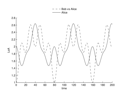
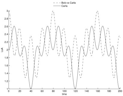
Figure 5: ($L_{1}=L_{2}=3$: Alice’s and Bob’s LoA’s vs. time with initial condition $(0,2)$ (left) and Carla’s and Bob’s LoA’s vs. time with initial condition $(2,3)$ (right). Periodic behaviours are observed.

The periodic behavior is clearly evident in both these plots. On the contrary, in Figure 6, we plot the solutions in the quasiperiodic case for the same $L_{1}$, $L_{2}$, $n_{12}(0)$, $n_{13}(0)$, $n_{2}(0)$ and $n_{3}(0)$ as above. The values of the parameters are $\lambda_{12}=\frac{1}{10}$, $\lambda_{13}=\frac{1}{8}$ and $\lambda_{1}\simeq 0.0889$, which satisfy condition (3.12) for $p=\sqrt{5}$ and $q=1$.

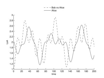
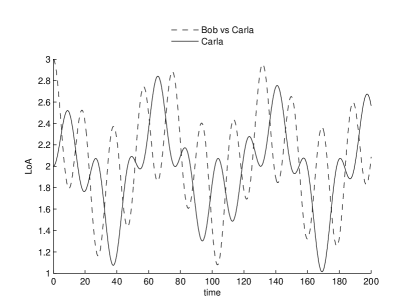
Figure 6: ($L_{1}=L_{2}=3$: Alice’s and Bob’s LoA’s vs. time with initial condition $(0,2)$ (left) and Carla’s and Bob’s LoA’s vs. time with initial condition $(2,3)$ (right). Quasiperiodic behaviours are observed.

3.1 Another generalization

A natural way to extend our previous Hamiltonian consists, in view of what we have done in Subsection 2.1, in introducing two different parameters $M_{\alpha}$, $\alpha=12,13$, which are able to describe the different (relative) reactions in the two interactions Alice–Bob and Carla–Bob. We also assume that Bob is not very interested in choosing Carla rather than Alice, as long as one of the two is attracted by him. For these reasons, the Hamiltonian looks now like

$$H=\lambda_{12}\left((a_{12}^{\dagger})^{M_{12}}\,a_{2}+a_{12}^{M_{12}}\,a_{2}^{\dagger}\right)+\lambda_{13}\left((a_{13}^{\dagger})^{M_{13}}\,a_{3}+a_{13}^{M_{12}}\,a_{3}^{\dagger}\right)+\lambda_{1}\left(a_{12}^{\dagger}\,a_{13}+a_{12}\,a_{13}^{\dagger}\right).$$

Also in this case an integral of motion does exist, and looks like

$$\tilde{J}:=N_{12}+N_{13}+M_{12}N_{2}+M_{13}N_{3},$$

which reduces to $J$ if $M_{12}=M_{13}=1$. The equations of motion also extend those given in (3.6), i.e.,

$$\left\{\begin{array}[]{ll}i\,\dot{a}_{12}(t)=\lambda_{12}\,M_{12}\,(a_{12}^{\dagger}(t))^{M_{12}-1}a_{2}(t)+\lambda_{1}\,a_{13}(t),\\ i\,\dot{a}_{13}(t)=\lambda_{13}\,M_{13}\,(a_{13}^{\dagger}(t))^{M_{13}-1}\,a_{3}(t)+\lambda_{1}\,a_{12}(t),\\ i\,\dot{a}_{2}(t)=\lambda_{12}\,a_{12}(t),\\ i\,\dot{a}_{3}(t)=\lambda_{13}\,a_{13}(t).\end{array}\right.$$ (3.17)

System (3.17) is nonlinear and can not be solved analytically unless if $M_{12}=M_{13}=1$, as shown before. Therefore, we adopt the same approach we have considered in our first model.

In particular, we take $L_{1}=L_{2}=2$, consider the orthonormal basis $\mathcal{F}=\left\{\varphi_{ijkl}\right\}$, where the indices $i,j,k,l$ run over the values 0,1,2 in such a way the sequence of four–digit numbers $ijkl$ (in base-3 numeral system) is sorted in ascending order, whereupon $dim(\mathcal{H}_{eff})=(L_{1}+1)^{2}(L_{2}+1)^{2}=81$. In such a situation, the unknowns $a_{12}(t)$, $a_{13}(t)$, $a_{2}(t)$ and $a_{3}(t)$ in the system (3.17) are square matrices of dimension 81, and their expression at $t=0$ are given by:

$$a_{12}(0)=\left(\begin{array}[]{lll}\mathbf{0}_{27}&\mathbf{0}_{27}&\mathbf{0}_{27}\\ 1\!\!1_{27}&\mathbf{0}_{27}&\mathbf{0}_{27}\\ \mathbf{0}_{27}&\sqrt{2}1\!\!1_{27}&\mathbf{0}_{27}\end{array}\right),\qquad a_{13}(0)=\left(\begin{array}[]{lll}\underline{x}&\mathbf{0}_{27}&\mathbf{0}_{27}\\ \mathbf{0}_{27}&\underline{x}&\mathbf{0}_{27}\\ \mathbf{0}_{27}&\mathbf{0}_{27}&\underline{x}\end{array}\right),$$

$$a_{2}(0)=\left(\begin{array}[]{lll}\underline{y}&\mathbf{0}_{27}&\mathbf{0}_{27}\\ \mathbf{0}_{27}&\underline{y}&\mathbf{0}_{27}\\ \mathbf{0}_{27}&\mathbf{0}_{27}&\underline{y}\end{array}\right),\qquad a_{3}(0)=\left(\begin{array}[]{lll}\underline{z}&\mathbf{0}_{27}&\mathbf{0}_{27}\\ \mathbf{0}_{27}&\underline{z}&\mathbf{0}_{27}\\ \mathbf{0}_{27}&\mathbf{0}_{27}&\underline{z}\end{array}\right),$$

where

$$\underline{x}=\left(\begin{array}[]{lll}\mathbf{0}_{9}&\mathbf{0}_{9}&\mathbf{0}_{9}\\ 1\!\!1_{9}&\mathbf{0}_{9}&\mathbf{0}_{9}\\ \mathbf{0}_{9}&\sqrt{2}1\!\!1_{9}&\mathbf{0}_{9}\end{array}\right),\qquad \underline{y}=\left(\begin{array}[]{lll}\underline{y}_{1}&\mathbf{0}_{9}&\mathbf{0}_{9}\\ \mathbf{0}_{9}&\underline{y}_{1}&\mathbf{0}_{9}\\ \mathbf{0}_{9}&\mathbf{0}_{9}&\underline{y}_{1}\end{array}\right),$$

$$\underline{y}_{1}=\left(\begin{array}[]{lll}\mathbf{0}_{3}&\mathbf{0}_{3}&\mathbf{0}_{3}\\ 1\!\!1_{3}&\mathbf{0}_{3}&\mathbf{0}_{3}\\ \mathbf{0}_{3}&\sqrt{2}1\!\!1_{3}&\mathbf{0}_{3}\end{array}\right),\qquad \underline{z}=\left(\begin{array}[]{lll}\underline{z}_{1}&\mathbf{0}_{9}&\mathbf{0}_{9}\\ \mathbf{0}_{9}&\underline{z}_{1}&\mathbf{0}_{9}\\ \mathbf{0}_{9}&\mathbf{0}&\underline{z}_{1}\end{array}\right),$$

$$\underline{z}_{1}=\left(\begin{array}[]{lll}\underline{z}_{2}&\mathbf{0}_{3}&\mathbf{0}_{3}\\ \mathbf{0}_{3}&\underline{z}_{2}&\mathbf{0}_{3}\\ \mathbf{0}_{3}&\mathbf{0}_{3}&\underline{z}_{2}\end{array}\right),\qquad \underline{z}_{2}=\left(\begin{array}[]{lll}0&0&0\\ 1&0&0\\ 0&\sqrt{2}&0\end{array}\right).$$

Moreover, in order to consider a situation not very far from a linear one, we choose $M_{12}=1$, $M_{13}=2$, $\lambda_{1}=0.3$, $\lambda_{12}=0.2$, $\lambda_{13}=0.007$.

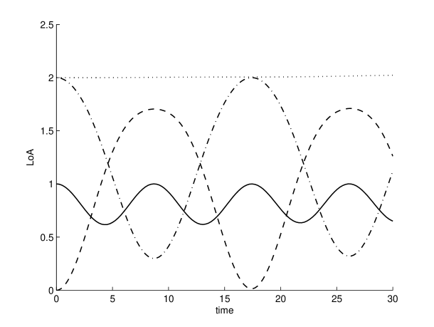
Figure 7: ($L_{\alpha}=2$, $M_{12}=1$, $M_{13}=2$ ($\alpha=12,13,2,3$): LoA vs. time of: Bob vs. Alice (continuous line), Bob vs. Carla (dashed line), Alice (dashed–dotted line), Carla (dotted line) with initial condition $(1,0,2,2)$. Periodic behaviours are observed.

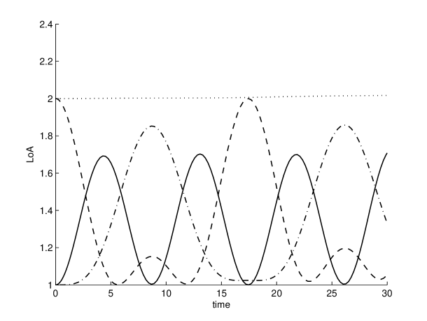
Figure 8: ($L_{\alpha}=2$, $M_{12}=1$, $M_{13}=2$ ($\alpha=12,13,2,3$): LoA vs. time of: Bob vs. Alice (continuous line), Bob vs. Carla (dashed line), Alice (dashed–dotted line), Carla (dotted line) with initial condition $(1,2,1,2)$. Periodic behaviours are observed.

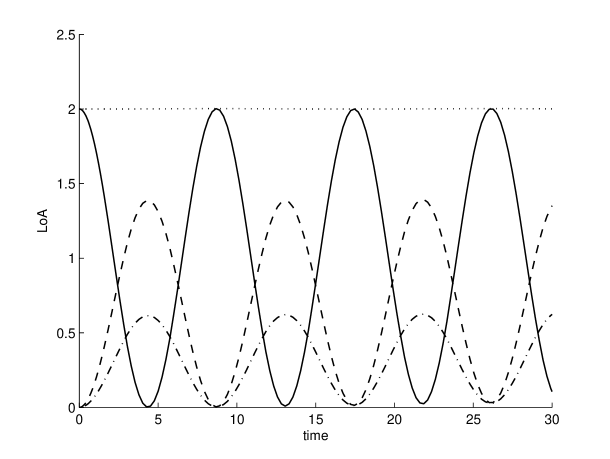
Figure 9: ($L_{\alpha}=2$, $M_{12}=1$, $M_{13}=2$ ($\alpha=12,13,2,3$): LoA vs. time of: Bob vs. Alice (continuous line), Bob vs. Carla (dashed line), Alice (dashed–dotted line), Carla (dotted line) with initial condition $(2,0,0,2)$. Periodic behaviours are observed.

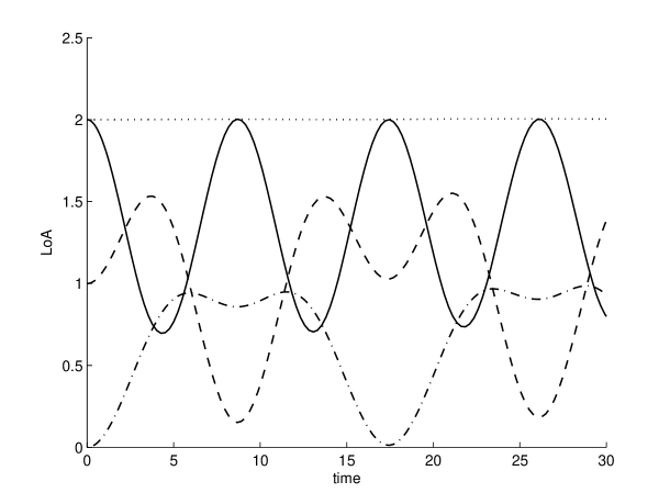
Figure 10: ($L_{\alpha}=2$, $M_{12}=1$, $M_{13}=2$ ($\alpha=12,13,2,3$): LoA vs. time of: Bob vs. Alice (continuous line), Bob vs. Carla (dashed line), Alice (dashed–dotted line), Carla (dotted line) with initial condition $(2,1,0,2)$. Periodic behaviours are observed.

The numerical integration has been performed by using once again the ode113 routine of MATLAB^®, and the existence of the integral of motion has been used in order to check the accuracy of the solutions.

The choice $\lambda_{13}=0.007$ has an immediate consequence, which is clearly displayed by the plots in figures 7-10. The time evolution of $N_{3}(t)$ is very slow and essentially trivial in the time interval where the system is numerically integrated: Carla keeps her initial status. This does not imply, however, that Bob does not change his LoA concerning Carla, as the figures 7-10 also clearly show. Another interesting feature, which is again due to the nonlinear aspect of the dynamics (and it was not present in the linear model), is related to the fact that, for certain time intervals, Bob’s LoA for both Alice and Carla can increase. This is, in a certain sense, unexpected: the Hamiltonian does not present any explicit ingredient responsible for this feature, which, in our opinion, appears just because of the nonlinearity of the interaction. Finally, we also notice that the figures 7-10 display a periodic behavior, even if no analytic proof of the existence of this periodicity was produced, up to now.

It is worth noticing that, contrarily to what happened in Section 2 (for certain initial conditions the dimension of $\mathcal{H}_{eff}$ needs to be increased in order to capture the right dynamics), all the numerical results obtained here suggest that, once the dimension of $\mathcal{H}_{eff}$ is fixed (and this is done when the initial conditions are given), the time evolution of the various LoA’s can be described inside that $\mathcal{H}_{eff}$, i.e., there is no need to enlarge the dimension of the effective Hilbert space. This could be related to our choice of the parameters, which, as already stated, produces a system with small nonlinear interactions. For this reason, we do not expect this to be a general feature of the model: on the contrary, we expect that, changing significantly the values of the parameters, the need for increasing the dimensionality of $\mathcal{H}_{eff}$ will arise also here. Further analysis in this direction is in progress.

4 Conclusions

In this paper we have shown how to use quantum mechanical tools in the analysis of dynamical systems which model a two– and a three–actor love relationship. Depending on the parameters which describe the system, linear or nonlinear differential equations are recovered, and exact or numerical solutions are found. These solutions show that a nontrivial dynamical behavior can be obtained, and a necessary and sufficient condition for the periodicity or quasiperiodicity of the solution in the linear love triangle model has been found, (3.12).

It is worth stressing that, despite the quantum framework adopted in this paper, all the observables relevant for the description of the models considered here commute among them and, for this reason, can be measured simultaneously and no Heisenberg uncertainty principle should be invoked for these operators.

A final comment is related to the oscillatory behavior recovered in this paper for the different LoA’s. Indeed, this is expected, due to the hamiltonian approach considered here. In a paper which is now in preparation, [17], one of us is considering the possibility of describing, using the same techniques, other processes in which some time decay may occur because of possible interactions of the lovers with the environment: this, we believe, could be a reasonable method to construct a more realistic model, where also different psychological mechanisms can be taken into account.

Appendix: A few results on the occupation number representation

We discuss here a few important facts in quantum mechanics and second quantization, paying not much attention to mathematical problems arising from the fact that the operators involved are quite often unbounded. More details can be found, for instance, in [18, 19].

Let $\mathcal{H}$ be an Hilbert space, and $B(\mathcal{H})$ the set of all the bounded operators on $\mathcal{H}$. Let $\mathcal{S}$ be our physical system, and $\mathcal{A}$ the set of all the operators useful for a complete description of $\mathcal{S}$, which includes the observables of $\mathcal{S}$. For simplicity, it is convenient to assume that $\mathcal{A}$ coincides with $B(\mathcal{H})$ itself, even if this is not always possible. This aspect, related to the importance of some unbounded operators within our scheme, will not be considered here, even because the Hilbert space $\mathcal{H}_{eff}$ considered in this paper is finite–dimensional, which implies that the operators in $\mathcal{A}$ are bounded matrices. The description of the time evolution of $\mathcal{S}$ is related to a self–adjoint operator $H=H^{\dagger}$ which is called the Hamiltonian of $\mathcal{S}$, and which in standard quantum mechanics represents the energy of $\mathcal{S}$. We will adopt here the so–called Heisenberg representation, in which the time evolution of an observable $X\in\mathcal{A}$ is given by

$$X(t)=e^{iHt}Xe^{-iHt},$$ (A.1)

or, equivalently, by the solution of the differential equation

$$\frac{dX(t)}{dt}=ie^{iHt}[H,X]e^{-iHt}=i[H,X(t)],$$ (A.2)

where $[A,B]:=AB-BA$ is the commutator between $A$ and $B$. The time evolution defined in this way is usually a one–parameter group of automorphisms of $\mathcal{A}$.

An operator $Z\in\mathcal{A}$ is a constant of motion if it commutes with $H$. Indeed, in this case, equation (A.2) implies that $\dot{Z}(t)=0$, so that $Z(t)=Z$ for all $t$.

In our paper a special role is played by the so–called canonical commutation relations (CCR): we say that a set of operators $\{a_{\ell},\,a_{\ell}^{\dagger},\ell=1,2,\ldots,L\}$ satisfy the CCR if the conditions

$$[a_{\ell},a_{n}^{\dagger}]=\delta_{\ell n}1\!\!1,\hskip 22.76219pt[a_{\ell},a_{n}]=[a_{\ell}^{\dagger},a_{n}^{\dagger}]=0$$ (A.3)

hold true for all $\ell,n=1,2,\ldots,L$. Here, $1\!\!1$ is the identity operator. These operators, which are widely analyzed in any textbook in quantum mechanics (see, for instance, [18]) are those which are used to describe $L$ different modes of bosons. From these operators we can construct $\hat{n}_{\ell}=a_{\ell}^{\dagger}a_{\ell}$ and $\hat{N}=\sum_{\ell=1}^{L}\hat{n}_{\ell}$, which are both self–adjoint. In particular, $\hat{n}_{\ell}$ is the number operator for the $\ell$-th mode, while $\hat{N}$ is the number operator of $\mathcal{S}$.

The Hilbert space of our system is constructed as follows: we introduce the vacuum of the theory, that is a vector $\varphi_{0}$ which is annihilated by all the operators $a_{\ell}$: $a_{\ell}\varphi_{0}=0$ for all $\ell=1,2,\ldots,L$. Then we act on $\varphi_{0}$ with the operators $a_{\ell}^{\dagger}$ and their powers:

$$\varphi_{n_{1},n_{2},\ldots,n_{L}}:=\frac{1}{\sqrt{n_{1}!\,n_{2}!\ldots n_{L}!}}(a_{1}^{\dagger})^{n_{1}}(a_{2}^{\dagger})^{n_{2}}\cdots(a_{L}^{\dagger})^{n_{L}}\varphi_{0},$$ (A.4)

$n_{l}=0,1,2,\ldots$ for all $l$. These vectors form an orthonormal set and are eigenstates of both $\hat{n}_{\ell}$ and $\hat{N}$: $\hat{n}_{\ell}\varphi_{n_{1},n_{2},\ldots,n_{L}}=n_{\ell}\varphi_{n_{1},n_{2},\ldots,n_{L}}$ and $\hat{N}\varphi_{n_{1},n_{2},\ldots,n_{L}}=N\varphi_{n_{1},n_{2},\ldots,n_{L}}$, where $N=\sum_{\ell=1}^{L}n_{\ell}$. Moreover, using the CCR we deduce that $\hat{n}_{\ell}\left(a_{\ell}\varphi_{n_{1},n_{2},\ldots,n_{L}}\right)=(n_{\ell}-1)(a_{\ell}\varphi_{n_{1},n_{2},\ldots,n_{L}})$ and $\hat{n}_{\ell}\left(a_{\ell}^{\dagger}\varphi_{n_{1},n_{2},\ldots,n_{L}}\right)=(n_{\ell}+1)(a_{l}^{\dagger}\varphi_{n_{1},n_{2},\ldots,n_{L}})$, for all $\ell$. For these reasons, the following interpretation is given: if the $L$ different modes of bosons of $\mathcal{S}$ are described by the vector $\varphi_{n_{1},n_{2},\ldots,n_{L}}$, this implies that $n_{1}$ bosons are in the first mode, $n_{2}$ in the second mode, and so on. The operator $\hat{n}_{\ell}$ acts on $\varphi_{n_{1},n_{2},\ldots,n_{L}}$ and returns $n_{\ell}$, which is exactly the number of bosons in the $\ell$–th mode. The operator $\hat{N}$ counts the total number of bosons. Moreover, the operator $a_{\ell}$ destroys a boson in the $\ell$–th mode, while $a_{\ell}^{\dagger}$ creates a boson in the same mode. This is why $a_{\ell}$ and $a_{\ell}^{\dagger}$ are usually called the annihilation and the creation operators.

The Hilbert space $\mathcal{H}$ is obtained by taking the closure of the linear span of all these vectors.

The vector $\varphi_{n_{1},n_{2},\ldots,n_{L}}$ in (A.4) defines a vector (or number) state over the algebra $\mathcal{A}$ as

$$\omega_{n_{1},n_{2},\ldots,n_{L}}(X)=\langle\varphi_{n_{1},n_{2},\ldots,n_{L}},X\varphi_{n_{1},n_{2},\ldots,n_{L}}\rangle,$$ (A.5)

where $\langle\,,\,\rangle$ is the scalar product in the Hilbert space $\mathcal{H}$. As we have discussed in [1, 2, 3, 4], these states are used to project from quantum to classical dynamics and to fix the initial conditions of the system considered.

References

• [1] F. Bagarello. An operatorial approach to stock markets. J. Phys. A, 39, 6823–6840, 2006.
• [2] F. Bagarello. Stock markets and quantum dynamics: a second quantized description. Physica A, 386, 283–302, 2007.
• [3] F. Bagarello. Simplified Stock markets described by number operators. Rep. Math. Phys., 63, 381–398, 2009.
• [4] F. Bagarello. A quantum statistical approach to simplified stock markets. Physica A, 388, 4397–4406, 2009.
• [5] S. H. Strogatz. Love affairs and differential equations. Mathematics Magazine, 61, 35, 1988.
• [6] S. H. Strogatz, Nonlinear Dynamics and Chaos. Addison–Wesley, 1994.
• [7] S. Rinaldi. Love dynamics: the case of linear couples. Appl. Math. Computation, 95, 181–192, 1998.
• [8] S. Rinaldi. Laura and Petrarch. An intriguing case of cyclical love dynamics. SIAM J. Appl. Math., 58, 1205–1221, 1998.
• [9] J. C. Sprott. Dynamical models of love. Nonlinear Dynamics, Psychology and Life Sciences, 8, 303–314, 2004.
• [10] J. C. Sprott. Dynamical models of happiness. Nonlinear Dynamics, Psychology and Life Sciences, 9, 23–36, 2005.
• [11] J. M. Gottman, J. D. Murray, C. C. Swanson, R. Tyson, K. R. Swanson. The mathematics of Marriage- Dynamics nonlinear models, The MIT Press, 2002.
• [12] B. E. Baaquie. Quantum Finance, Cambridge University Press (2004)
• [13] M. Schaden. A quantum approach to stock price fluctuations, Physica A, 316, 511 (2002)
• [14] M. Arndt, T. Juffmann, V. Vedral. Quantum physics meets biology, HFSP J. 2009; 3(6): 386400.
• [15] D. Aerts, S. Aerts, L. Gabora. Experimental Evidence for Quantum Structure in Cognition. Lecture Notes In Artificial Intelligence; Vol. 5494, Proceedings of the 3rd International Symposium on Quantum Interaction, 59-70, 2009.
• [16] D. Aerts, B. D’Hooghe, E. Haven, Quantum Experimental Data in Psychology and Economics , arXiv: 1004.2529 [physics.soc-ph]
• [17] F. Bagarello. Damping in quantum love affairs. In preparation.
• [18] E. Merzbacher. Quantum Mechanics. Wiley, New York, 1970.
• [19] M. Reed, B. Simon. Methods of Modern Mathematical Physics, I, Academic Press, New York, 1980.
• [20] L. F. Shampine, M. K. Gordon. Computer Solution of Ordinary Differential Equations: the Initial Value Problem, W. H. Freeman, San Francisco, 1975.