Queue-Aware Distributive Resource Control for Delay-Sensitive Two-Hop MIMO Cooperative Systems

Abstract

In this paper, we consider a queue-aware distributive resource control algorithm for two-hop MIMO cooperative systems. We shall illustrate that relay buffering is an effective way to reduce the intrinsic half-duplex penalty in cooperative systems. The complex interactions of the queues at the source node and the relays are modeled as an average-cost infinite horizon Markov Decision Process (MDP). The traditional approach solving this MDP problem involves centralized control with huge complexity. To obtain a distributive and low complexity solution, we introduce a linear structure which approximates the value function of the associated Bellman equation by the sum of per-node value functions. We derive a distributive two-stage two-winner auction-based control policy which is a function of the local CSI and local QSI only. Furthermore, to estimate the best fit approximation parameter, we propose a distributive online stochastic learning algorithm using stochastic approximation theory. Finally, we establish technical conditions for almost-sure convergence and show that under heavy traffic, the proposed low complexity distributive control is global optimal.

I Introduction

Cooperative relay communication has been a hot research topic in both the academia [1, 2] and the industry [3, 4] because it could exploit the broadcast nature of wireless communication to achieve cooperative diversity. One potential issue of cooperative communication is the half-duplex penalty in the relay nodes. There have been some recent works to address the half-duplex issue in cooperative relay systems. For example, complex echo cancelation technique is used at the relay to cancel the coupled interference from the transmitting path [5, 6]. However, these works all focused at the physical layer signal processing. In [7], the authors exploit special topology and proposed some relay protocols to get rid of the half-duplex penalty. Moreover, this approach depends heavily on the locations of the relays and it cannot be extended to general relay channel. In this paper, we are interested to explore a system level solution to deal with the half-duplex issue. We consider a simple MIMO cooperative relay system with a multi-antenna source node (Src), $M$ multi-antenna relay nodes (RS) and a multi-antenna destination node (Dst). We shall illustrate that relay buffering can be utilized to significantly reduce the intrinsic half-duplex penalty. Since buffering is involved, it is important to consider not only the throughput performance but also the associated end-to-end delay performance. As a result, we shall focus on delay-optimal resource control for the two-hop protocol in MIMO cooperative relay systems.

Delay-optimal resource control in cooperative relay system is a very difficult problem. Most of the existing works have assumed infinite backlogs of information and focus on optimizing the throughput performance only. A systematic approach is to model the delay-optimal control as Markov Decision Process (MDP) [8, 9]. However, there is a well-known issue of the curse of dimensionality and brute force value iteration or policy iteration could not give simple implementable solutions. For multi-hop systems, there is a unique challenge concerning the complex interactions of buffers at the source node and the $M$ RS nodes and the existing solutions for single-hop systems cannot be extended easily to deal with this situation. There are a few recent works that considered queue dynamics in relay systems [10, 11]. However, these works have focused on the characterization of the stability region and throughput optimal control. The question of delay-optimal control for cooperative relay system remains to be open. In addition, another important technical challenge is the distributive implementation consideration. For instance, the entire system state could be characterized by the global CSI (CSI among every pair of nodes in the system) as well as the global QSI (QSI of every buffer in the system). Brute-force solution of the MDP will yield a control policy that is adaptive to the global CSI and global QSI. This poses a huge implementation challenges because these global system state information are distributed locally at each of the source and relay nodes.

In this paper, we shall address the above challenges as follows. We shall first formulate the delay-optimal resource control policy (such as the power control and RS selection) as an average-cost infinite horizon Markov Decision Process (MDP). To alleviate the curse of dimensionality, and to obtain a distributive and low complexity solution, we first introduce a per-node value function to approximate the value function of the associated Bellman equation. Based on the per-node value function, we derive a distributive two-stage two-winner auction-based control policy, which is a function of the local CSI and local QSI. The per-node value function is obtained via a distributive online stochastic learning algorithm, which requires local CSI and local QSI only. The proposed online stochastic learning is quite different from the conventional reinforced learning [12] in mainly two ways: (1) We are dealing with constrained MDP (CMDP) and our online iterative solution updates both the value function and the Lagrange multipliers (LM) simultaneously; (2) The control action is determined from the per-node value function of all the nodes via a per-slot auction mechanism. Therefore, the algorithm dynamics of the per-node online learning is not a contraction mapping and hence, standard convergence proof using fixed point theorem cannot be applied in our case directly. Using the technique of separation of different time scales, we establish technical conditions for the almost sure convergence of the proposed distributive stochastic learning. We also show that the proposed low complexity distributive solution is asymptotically global optimal under heavy traffic loading. Finally, we demonstrate by simulation that the proposed scheme has significant performance gain over various baselines (such as conventional CSIT-only control and the throughput-optimal control (in stability sense)) with low complexity $\mathcal{O}(M)$ and low signaling overhead.

II System Models

II-A System Architecture and MIMO Relay Physical Layer Model

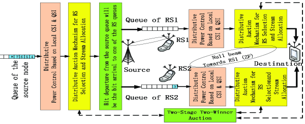
Figure 1: Illustration of the two-hop MIMO cooperative system with a multi-antenna source node, 2 multi-antenna RS nodes and a multi-antenna destination node. By exploiting buffers at the 2 MIMO RSs, the S-R link (source node to RS1) and R-D link (RS2 to destination node) can deliver packets simultaneously without interfering with each other using signal processing techniques (with appropriate precoder and decorrelator designs). Thus, by exploiting relay buffering, we could substantially reduce the intrinsic penalty associated with half duplex relays.

We consider a two-hop multi-antenna cooperative relay communication system with one multi-antenna source node ($N_{T}$ antennas), $M$ multi-antenna half-duplex relay stations (RS, each with $N_{R}$ antennas) and one multi-antenna destination node ($N_{T}$ antennas), as illustrated in Fig. 1. The source node cannot deliver packets directly to the destination node due to limited coverage and the cooperative RSs are deployed to extend the source node’s coverage.

Denote the Rx-RS and the Tx-RS as the $m$-th RS and the $n$-th RS for notation simplicity. Let $N_{SR}$ and $N_{RD}$ be the number of data streams transmitted in the S-R link and the R-D link respectively, where we require $N_{RD}=\min(N_{T},N_{R}-N_{SR})$ for simultaneous interference-free transmission. We shall illustrate the signal model of the S-R_m link and the R_n-D link as follows:

• S-R_m link: Let $\mathbf{X}_{S}\in C^{N_{SR}\times 1}$ and $\mathbf{F}_{S}\in C^{N_{T}\times N_{SR}}$ be the symbol vector and the precoder matrix of the source node respectively, $\mathbf{G}_{m}\in C^{N_{SR}\times N_{R}}$ be the decorrelator matrix at the $m$-th RS node, the $N_{SR}\times 1$ post-processing symbol vector at the $m$-th RS is given by $\mathbf{Y}_{m}=\mathbf{G}_{m}\mathbf{H}_{S,m}\mathbf{F}_{S}\mathbf{X}_{S}+\mathbf{Z}_{S,m}$, where $\mathbf{H}_{S,m}\in C^{N_{R}\times N_{T}}$ is the zero-mean unit variance i.i.d. complex Gaussian fading matrix from the source node to the $m$-th RS, $\mathbf{Z}_{S,m}\in C^{N_{SR}\times 1}$ is the zero-mean unit variance complex Gaussian channel noise.

• R_n-D link: Let $\mathbf{X}_{n}\in C^{N_{RD}\times 1}$ and $\mathbf{F}_{n}\in C^{{\color[rgb]{0,0,0}N_{R}}\times N_{RD}}$ be the transmit symbol vector and the precoder of the $n$-th RS respectively, the ${\color[rgb]{0,0,0}N_{T}}\times 1$ received symbol vector at the destination node is given by $\mathbf{Y}_{D}=\mathbf{H}_{n,D}\mathbf{F}_{n}\mathbf{X}_{n}+\mathbf{Z}_{n,D}$, where $\mathbf{H}_{n,D}\in C^{N_{T}\times N_{R}}$ is complex Gaussian fading matrix from the $n$-th RS to the destination node, $\mathbf{Z}_{n,D}\in C^{N_{T}\times 1}$ is the complex Gaussian channel noise.

In this paper, the resource control is performed distributively on each RS and therefore, we define the local channel state information (CSI) available at each RS as follows. For the $m$-th RS, there are two types of local CSI, namely the type-I local CSI and type-II local CSI as illustrated in Fig. 2. The type-I and type-II local CSI of the $m$-th RS are denoted by $\mathbf{H}_{m}^{I}=\{\mathbf{H}_{S,m}\}$ and $\mathbf{H}_{m}^{II}=\{\mathbf{H}_{m,D}\}\cup\{\mathbf{H}_{m,n}|n\neq m,1\leq n\leq M\}$, respectively. For notation convenience, let $\mathbf{H}_{m}=\mathbf{H}_{m}^{I}\cup\mathbf{H}_{m}^{II}$ be the local CSI at the $m$-th RS and $\mathbf{H}=\cup_{m=1}^{M}\ \mathbf{H}_{m}$ be the global CSI (GCSI) of the system. Moreover, the assumption on the channel is summarized below:

Assumption 1 (Assumption on Channel Fading)

We assume the channel fading elements in the global CSI $\mathbf{H}$ are i.i.d. $\mathcal{CN}(0,1)$. The CSI is quasi-static within a frame but i.i.d. between frames.

We assume strong channel coding is used and hence, the maximum achievable data rate is given by the instantaneous mutual information. If the source node transmits $R_{S,m}$ information bits to the $m$-th RS in the current frame, the frame will be successfully received if $R_{S,m}\leq\tau\log_{2}\det\big{[}\mathbf{I}+\mathbf{G}_{m}\mathbf{H}_{S,m}\mathbf{F}_{S}\mathbf{F}_{S}^{{\dagger}}\mathbf{H}_{S,m}^{{\dagger}}\mathbf{G}_{m}^{{\dagger}}\big{]}$, where ^† denotes the matrix conjugate transpose and $\tau$ is the frame duration. Similarly, the destination node could successfully decode a frame with $R_{n,D}$ information bits (transmitted from the $n$-th RS) if $R_{n,D}\leq\tau\log_{2}\det\big{[}\mathbf{I}+\mathbf{H}_{n,D}\mathbf{F}_{n}\mathbf{F}_{n}^{{\dagger}}\mathbf{H}_{n,D}^{{\dagger}}\big{]}$.

II-B Buffered Decode and Forward

Although the RS nodes are half-duplex relays, it is possible to reduce the system half-duplex penalty by exploiting buffers at the half-duplex RSs. Specifically, the source node could transmit a packet to the $m$-th RS (denoted as the Rx-RS) and at the same time, the $n$-th RS (denoted as the Tx-RS) transmits its buffered packet to the destination node without interfering the Rx-RS. This is possible by means of precoder-decorrelator designs at the source node, Rx-RS ($m$-th RS) and the Tx-RS ($n$-th RS). Let $p_{S,m}$ and $p_{n,D}$ denote the total transmit power at the source node for the S-R_m link and the Tx-RS ($n$-th RS) for the R_n-D link, respectively. For any given $N_{SR}$, $p_{S,m}$ for the S-R_m link as well as $N_{RD}$, $p_{n,D}$ for the R_n-D link (where $N_{RD}=\min(N_{T},N_{R}-N_{SR})$ implicitly), the decorrelator and precoder designs are elaborated below.

• Precoder and Decorrelator Design of the S-R_m Link at the Rx-RS Node: The precoder at the source node ($\mathbf{F}_{S}$) and the decorrelator at the Rx-RS node ($\mathbf{G}_{m}$) are chosen to optimize the mutual information of the S-R_m link subject to the transmit power constraint as follows:

  $$\{\mathbf{G}_{m}^{*}(N_{SR}),\mathbf{F}_{S}^{*}(N_{SR},p_{S,m})\} = \arg\max_{\mathbf{F}_{S},\mathbf{G}_{m}}\log_{2}\det\Big{[}\mathbf{I}+\mathbf{G}_{m}(N_{SR})\mathbf{H}_{S,m}\mathbf{F}_{S}\mathbf{F}_{S}^{{\dagger}}\mathbf{H}_{S,m}^{{\dagger}}\mathbf{G}_{m}^{{\dagger}}(N_{SR})\Big{]}$$ (1)

  $$s.t. tr(\mathbf{F}_{S}\mathbf{F}_{S}^{{\dagger}})=p_{S,m}\quad\mbox{(Transmit power constraint)}.$$

  Let $\mathbf{H}_{S,m}=\mathbf{U}_{S,m}\mathbf{\Sigma}_{S,m}\mathbf{V}_{S,m}^{{\dagger}}$ be the SVD decomposition of channel matrix $\mathbf{H}_{S,m}$, where the singular values in $\mathbf{\Sigma}_{S,m}$ are sorted in a decreasing order along the diagonal, $\mathbf{U}_{S,m}=[\mathbf{u}_{S,m}^{1},...,\mathbf{u}_{S,m}^{N_{R}}]$ and $\mathbf{V}_{S,m}=[\mathbf{v}_{S,m}^{1},...,\mathbf{v}_{S,m}^{N_{T}}]$. Using standard optimization techniques [14], the source precoder $\mathbf{F}_{S}^{*}$ is given by

  $$\mathbf{F}_{S}^{*}(N_{SR},p_{S,m})=[\mathbf{v}_{S,m}^{1},...,\mathbf{v}_{S,m}^{N_{SR}}]\times diag\Big{\{}\frac{1}{\lambda_{S,m}}-\frac{1}{\eta_{S,m}^{1}},...,\frac{1}{\lambda_{S,m}}-\frac{1}{\eta_{S,m}^{N_{SR}}}\Big{\}},$$ (2)

  where $\eta_{S,m}^{1}\geq\eta_{S,m}^{2}...\geq\eta_{S,m}^{N_{SR}}$ are the first $N_{SR}$ singular values of channel matrix $\mathbf{H}_{S,m}$, $\lambda_{S,m}$ is the Lagrange multiplier corresponding to the transmit power constraint in (1). The decorrelator $\mathbf{G}_{m}^{*}$ is given by

  $$\mathbf{G}_{m}^{*}(N_{SR})=[\mathbf{u}_{S,m}^{1},...,\mathbf{u}_{S,m}^{N_{SR}}]^{{\dagger}}.$$ (3)

• Precoder Design of the R_n-D Link at the Tx-RS Node: Similarly, given the decorrelator $\mathbf{G}_{m}^{*}$ in (3), the precoder at the Tx-RS node $\mathbf{F}_{n}\in C^{N_{RD}\times N_{R}}$ is selected to maximize R-D link mutual information subject to the transmit power constraint and the interference nulling constraint (at the Rx-RS node) as follows:

  $$\mathbf{F}_{n}^{*}(N_{RD},p_{n,m}) = \arg\max_{\mathbf{F}_{n}}\log_{2}\det\Big{[}\mathbf{I}+\mathbf{H}_{n,D}\mathbf{F}_{n}\mathbf{F}_{n}^{{\dagger}}\mathbf{H}_{n,D}^{{\dagger}}\Big{]}$$ (5)

  $$s.t. \mathbf{G}_{m}^{*}(N_{SR})\mathbf{H}_{n,m}\mathbf{F}_{n}=0\quad\mbox{(Interference nulling constraint)}$$

  $$tr(\mathbf{F}_{n}\mathbf{F}_{n}^{{\dagger}})=p_{n,D}\quad\mbox{(Transmit power constraint)}$$

  The interference nulling constraint in (5) is to allow simultaneously active R-D and S-R links using half-duplex RSs. Let $\mathbf{H}_{n,D}\times null(\mathbf{G}_{m}\mathbf{H}_{n,m})=\mathbf{U}_{n,D}\mathbf{\Sigma}_{n,D}\mathbf{V}_{n,D}^{{\dagger}}$ be the SVD decomposition, where the singular values in $\mathbf{\Sigma}_{n,D}$ are sorted in a decreasing order along the diagonal, $null(\mathbf{G}_{m}\mathbf{H}_{n,m})$ denotes the null space of matrix $\mathbf{G}_{m}\mathbf{H}_{n,m}$ and $\mathbf{V}_{n,D}=[\mathbf{v}_{n,D}^{1},...,\mathbf{v}_{n,D}^{N_{R}-N_{SR}}]$. Using standard optimization techniques [14], the precoder at the Tx-RS ($\mathbf{F}_{n}^{*}$) is given by:

  $$\mathbf{F}_{n}^{*}(N_{RD},p_{n,m})=[\mathbf{v}_{S,n}^{1},...,\mathbf{v}_{S,n}^{N_{RD}}]\times diag\Big{\{}\frac{1}{\lambda_{n,D}}-\frac{1}{\eta_{n,D}^{1}},...,\frac{1}{\lambda_{n,D}}-\frac{1}{\eta_{n,D}^{N_{RD}}}\Big{\}},$$ (6)

  where $\eta_{n,D}^{1}\geq\eta_{n,D}^{2}...\geq\eta_{S,m}^{N_{RD}}$ are the first $N_{RD}$ singular values of channel matrix $\mathbf{H}_{n,D}\times null(\mathbf{G}_{m}\mathbf{H}_{n,m})$, $\lambda_{n,D}$ is the Lagrange multiplier corresponding to the power constraint in (5).

II-C Bursty Source Model and Queue Dynamics

There is one queue in the source node and one queue in each of the $M$ RSs respectively for the storage of received information bits. Let $N_{Q}$ be the maximum buffer size (number of bits) for the buffers in the source node and all the RSs. Let $X(t)$ indicates the number of new information bits arrival in the $t$-th frame at the source node. The assumption on the bit arrival process is given below:

Assumption 2 (Assumption on Arrival Process)

We assume $X(t)$ is i.i.d. over frames based on a general distribution $f_{X}(x)$ with $\mathbb{E}[X(t)]=\lambda_{S}$ and the information bits arrive at the end of each frame.

Moreover, let $Q_{S}(t)$ and $Q_{m}(t)$ denote the number of information bits in the source node’s queue and the $m$-th RS’s queue ($1\leq m\leq M$) at frame $t$. We assume each RS has the knowledge of its own queue length and the source node’s queue length. Thus, the local QSI of the $m$-th RS is $\big{(}Q_{S}(t),Q_{m}(t)\big{)}$. $\mathbf{Q}(t)=\big{(}Q_{S}(t),Q_{1}(t),\cdots,Q_{M}(t)\big{)}$ denotes the global queue state information (GQSI) at frame $t$.

The overall system queue dynamics at the source node and the RSs are summarized below.

• If the source node successfully delivers $R_{S,m}(t)$ information bits to the $m$-th RS at frame $t$, then $Q_{S}(t+1)=\min\left\{\max\{Q_{S}(t)-R_{S,m}(t),0\}+X(t),N_{Q}\right\}$ and $Q_{m}(t+1)=\min\left\{Q_{m}(t)+R_{S,m}(t),N_{Q}\right\}$.

• If the source node fails to deliver any information bit to the RSs , then $Q_{S}(t+1)=\min\left\{Q_{S}(t)+X(t),N_{Q}\right\}$.

• If the $n$-th RS successfully delivers $R_{n,D}(t)$ information bits to the destination at frame $t$, then $Q_{n}(t+1)=\max\{Q_{n}(t)-R_{n,D}(t),0\}$.

Remark 1

Each information bit delivered from the source node will be received by one of the RSs and different RSs may have different information bits in the buffer. When the source node is to deliver information bits to one RS, selecting different RSs with different buffer lengths may have different effects on the average packet delay of the system. Therefore, not only the CSI of all S-R links but also the QSI of all RSs should be considered in directing the source node’s transmission. Such coupling on the system QSI is a unique challenge in delay-optimal control of multi-hop systems. Fig. 1 shows the top level architecture illustrating the interactions among all the queues in the two-hop cooperative system.

II-D Distributive Contention Protocol

Based on the BDF in Section II-B, we still need to determine (a) which RS should be the Rx-RS ($m^{*}$), (b) which RS should be the Tx-RS ($n^{*}$) and (c) the number of data streams transmitted by the source node ($N_{SR}^{*}$) and the Tx-RS ($N_{RD}^{*}$). Due to the decentralized control requirement, we shall propose a two-stage two-winner auction mechanism for distributive contention resolution.

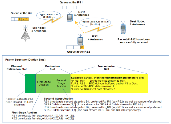
Figure 2: Illustration of an example of bidding protocol for a 2-RS system.

Figure 2 illustrates an example of bidding protocol for a 2-RS system. As a result, the RS selection and data stream allocation procedure can be parameterized by a bidding vector $\big{\{}\big{(}{\color[rgb]{0,0,0}A_{m}(0),...,A_{m}(\min(N_{T},N_{R}))}\big{)},$ $B_{m})|\forall m\big{\}}$. We shall refer the bidding vector as the RS selection and data stream allocation policy in the rest of the paper.

II-E Optimization Objective and Control Policy

Definition 1 (Distributive Stationary Control Policy)

A distributive stationary control policy $\Pi=\{\Pi^{m}|1\leq m\leq M\}$ is a collection of stationary control policies $\Pi^{m}$ at the $m$-th RS, where $\Pi^{m}=\{\Pi^{m}_{p},\Pi^{m}_{A},\Pi^{m}_{B}\}$ includes the power allocation policy of S-R link and R-D link $\Pi_{p}^{m}$, the first-stage and second-stage bidding policy $\Pi_{A}^{m}$ and $\Pi_{B}^{m}$. Specifically,

$$\Pi^{m}_{p}(S_{m})=\Big{\{}p_{S,m}(N_{SR}),p_{m,D}(N_{RD}):N_{SR},N_{RD}=0,1,\cdots,\min(N_{T},N_{R})\Big{\}}\triangleq\mathbf{p}_{m}$$ (7)

$$\Pi^{m}_{A}(S_{m})=\Big{\{}A_{m}(N_{SR})|N_{SR}=0,1,...,\min(N_{T},N_{R})\Big{\}}\triangleq\mathbf{A}_{m}$$ (8)

$$\Pi^{m}_{B}(S_{m},\cup_{m^{\prime}=1}^{M}\mathbf{A}_{m^{\prime}})=\Big{\{}B_{m},I_{m},(N_{SR,m},N_{RD,m})|N_{RD}=\min(N_{T},N_{R}-N_{SR})\Big{\}}\triangleq\mathbf{B}_{m}$$ (9)

for $m=1,2,...,M$, where $p_{S,m}(N_{SR})$ is the total transmit power allocation at the source node for the S-R link with $N_{SR}$ data streams, $p_{m,D}(N_{RD})$ is the total transmit power allocation at the Tx-RS for the R-D link with $N_{RD}$ data streams.

Denote the local system state of the $m$-th RS as $S_{m}=(Q_{S},Q_{m},\mathbf{H}_{m})$ ($1\leq m\leq M$). Therefore, the global system state is given by $\mathbf{S}=\cup_{m=1}^{M}\ S_{m}=(\mathbf{Q},\mathbf{H})$.

Remark 2 (Distributive Consideration of Stationary Control Policy $\Pi$ in Definition 1)

The stationary control policy $\Pi=\{\Pi^{m}|1\leq m\leq M\}$ is distributive in the sense that the policy $\Pi^{m}$ at each RS $m$ only depends on the local system state ${\color[rgb]{0,0,0}S_{m}}$ and the broadcast bidding information available at RS $m$. Thus, for notation simplicity, we shall omit the bidding information when the meaning is clear, i.e. we shall use $\Pi^{m}({\color[rgb]{0,0,0}S_{m}})=\{\Pi^{m}_{p}({\color[rgb]{0,0,0}S_{m}}),\Pi^{m}_{A}({\color[rgb]{0,0,0}S_{m}}),\Pi^{m}_{B}({\color[rgb]{0,0,0}S_{m}})\}$ in the rest of the paper.

A stationary control policy $\Pi$ induces a joint distribution for the random process $\{\mathbf{S}(t)\}$. Under Assumption 1 and 2, $\mathbf{S}(t+1)$ only depends on $\mathbf{S}(t)$ and actions at frame $t$, and hence the induced random process $\{\mathbf{S}(t)\}$ for a given control policy $\Pi$ is Markovian with the following transition probability:

$$\Pr\big{[}\mathbf{S}(t+1)\big{|}\mathbf{S}(t),\Pi\big{(}\mathbf{S}(t)\big{)}\big{]}=\Pr\big{[}\mathbf{H}(t+1)\big{]}\Pr\big{[}\mathbf{Q}(t+1)\big{|}\mathbf{S}(t),\Pi\big{(}\mathbf{S}(t)\big{)}\big{]},$$ (10)

where the equality is because of Assumption 1 and the queue dynamics transition probability $\Pr\big{[}\mathbf{Q}(t+1)\big{|}\mathbf{S}(t),\Pi\big{(}\mathbf{S}(t)\big{)}\big{]}$ is given by

$$\Pr\big{[}\mathbf{Q}(t+1)\big{|}\mathbf{S}(t),\Pi\big{(}\mathbf{S}(t)\big{)}\big{]}$$ (11)

$$= \begin{cases}\Pr\big{[}X(t)=Q_{S}(t+1)-[Q_{S}(t)-{\color[rgb]{0,0,0}R_{S,m^{*}}}(t)]^{+}\big{]},&\text{if }Q_{m}(t+1)=Q_{m}(t)\ (\forall m\neq m^{*},n^{*})\\ \quad\quad\text{and }Q_{m^{*}}(t+1)=\min\{Q_{m^{*}}(t)+R_{S,m^{*}}(t),N_{Q}\},&Q_{n^{*}}(t+1)=\max\{Q_{n^{*}}(t)-R_{n^{*},D}(t),0\}\\ 0,&\text{otherwise}\end{cases}$$

Given a unichain policy $\Pi$, the induced Markov chain $\{\mathbf{S}(t)\}$ is ergodic and there exists a unique steady state distribution $\pi_{S}$[8] . Therefore, we have the average end-to-end delay of the two-hop cooperative RS system summarized in the following lemma:

Lemma 1 (Average End-to-End Delay)

For small average packet drop rate constraint $D$, the average end-to-end delay of the two-hop cooperative RS system is given by

$$\overline{T}(\Pi)=\lim\limits_{T\rightarrow\infty}\frac{1}{T}\sum_{t=1}^{T}\mathbf{E}^{\Pi}\Big{[}\frac{\sum_{m=S}^{M}Q_{m}(t)}{\lambda_{S}}\Big{]}=\mathbf{E}_{\pi_{S}}\Big{[}\frac{\sum_{m=S}^{M}Q_{m}}{\lambda_{S}}\Big{]}$$ (12)

where $m=S,1,2,...,M$ in the equation, $\mathbf{E}_{\pi_{S}}$ means taking the expectation with respect to the induced steady state distribution $\pi_{S}$ (induced by the unichain control policy $\Pi$) and $\lambda_{S}$ is the average number of arrival bits per frame at the source node.

Proof:

Please refer to Appendix A. ∎

Similarly, the source node’s average drop rate constraint, the source node’s average power constraint and each RS $m$’s average power constraint are given by

$$\overline{D}(\Pi)=\lim\limits_{T\rightarrow\infty}\frac{1}{T}\sum_{t=1}^{T}\mathbf{E}^{\Pi}\Big{[}\mathbf{I}[Q_{S}(t)=N_{Q}]\Big{]}=\mathbf{E}^{\Pi}_{\pi_{\mathbf{S}}}\Big{[}\mathbf{I}[Q_{S}=N_{Q}]\Big{]}\leq D$$ (13)

$$\overline{P}_{S}(\Pi)=\lim\limits_{T\rightarrow\infty}\frac{1}{T}\sum_{t=1}^{T}\mathbf{E}^{\Pi}\Big{[}\sum_{m=1}^{M}\sum_{i=1}^{N_{\min}}I_{S,m}^{i}(t)p_{S,m}(i)(t)\Big{]}=\mathbf{E}_{\pi_{\mathbf{S}}}^{\Pi}\Big{[}\sum_{m=1}^{M}\sum_{i=1}^{N_{\min}}I_{S,m}^{i}p_{S,m}(i)\Big{]}\leq P_{S}$$ (14)

$$\overline{P}_{m}(\Pi)=\lim\limits_{T\rightarrow\infty}\frac{1}{T}\sum_{t=1}^{T}\mathbf{E}^{\Pi}\Big{[}\sum_{i=1}^{N_{\min}}I_{m,D}^{i}(t)p_{m,D}^{i}(t)\Big{]}=\mathbf{E}_{\pi_{\mathbf{S}}}\Big{[}\sum_{i=1}^{N_{\min}}I_{m,D}^{i}p_{m,D}^{i}\Big{]}\leq P_{R},1\leq m\leq M$$ (15)

where $N_{\min}=\min(N_{T},N_{R})$, $I_{S,m}^{i}=\mathbf{I}[m=m^{*}]\mathbf{I}[i=N_{SR}^{*}]$ and $I_{m,D}^{i}=\mathbf{I}[m=n^{*}]\mathbf{I}[i=N_{RD}^{*}]$.

III Constrained Markov Decision Problem Formulation

In this section, we shall formulate the delay-optimal problem as an infinite horizon average cost constrained Markov Decision Problem (CMDP) and discuss the general solution.

III-A CMDP Formulation

The goal of the controller is to choose an optimal stationary feasible unichain policy $\Pi^{*}$ that minimizes the average end-to-end transmission delay in (12). Specifically, the delay-optimal control problem is summarized below.

Problem 1 (Delay-Optimal Control Problem for MIMO Relay System)

Find a feasible stationary unichain policy $\mathbf{\Pi}=(\Pi^{1},...,\Pi^{M})$ such that the average end-to-end delay is minimized subject to the average drop rate constraint at the source node and the average power constraint at the source node and each RS node, i.e. $\min\limits_{\Pi}\ \overline{T}(\Pi)=\lim\limits_{T\rightarrow\infty}\frac{1}{T}\sum_{t=1}^{T}\mathbf{E}^{\Pi}\Big{[}\sum_{m=S}^{M}Q_{m}(t)\Big{]}\ s.t.\ \eqref{eqn:d-cont},\ \eqref{eqn:s-p-cont},\ \eqref{eqn:r-p-cont}$.

Problem 12 is an infinite horizon average cost constrained Markov Decision Problem (CMDP) [19] with system state space $\mathcal{S}=\{\mathbf{S}^{1},\mathbf{S}^{2},\cdots\}=\mathcal{Q}\times\mathcal{H}$ (where $\mathcal{Q}$ is the global QSI state space and $\mathcal{H}$ is the global CSI state space), action space $\mathcal{P}\times\mathcal{A}\times\mathcal{B}$ (where $\mathcal{P}=\{\forall\mathbf{p}_{m}|\forall m\}$ is power allocation action space, $\mathcal{A}=\{\forall\mathbf{A}_{m}|\forall m\}$ is the first-stage bidding action space and $\mathcal{B}=\{\forall\mathbf{B}_{m}|\forall m\}$ is the second-stage bidding action space), transition kernel given by (10), and the per-stage cost function $d\big{(}\mathbf{S},\Pi(\mathbf{S})\big{)}=\sum_{m=S}^{M}Q_{m}$.

III-B Lagrangian Approach for the CMDP

The CMDP in Problem 12 can be converted into unconstrained MDP by the Lagrange theory [14]. For any vector of Lagrange multiplier (LM) $\gamma=[\gamma_{S,d},\gamma_{S,p},\gamma_{1,p},...,\gamma_{M,p}]^{T}$, we define the Lagrangian as $L(\Pi,\gamma)=\lim\limits_{T\rightarrow+\infty}\frac{1}{T}\sum_{t=1}^{T}\mathbf{E}^{\Pi}_{\mathbf{S}}\Big{[}g\Big{(}\mathbf{S}(t),\Pi\big{(}\mathbf{S}(t)\big{)},\gamma\Big{)}\Big{]}$, where

$$g\big{(}\mathbf{S},\Pi\big{(}\mathbf{S}\big{)},\gamma\big{)}=Q_{S}+\gamma_{S,p}\sum_{m=1}^{M}\sum_{i=1}^{N_{\min}}I_{S,m}^{i}p_{S,m}(i)+\gamma_{S,d}\mathbf{I}[Q_{S}=N_{Q}]+\sum_{m=1}^{M}\Big{[}Q_{m}+\gamma_{m,p}\sum_{i=1}^{N_{\min}}I_{m,D}^{i}p_{m,D}(i)\Big{]}.$$

Therefore, the corresponding unconstrained MDP for a particular vector of LMs $\gamma$ is given by

$$G(\gamma)=\min_{\Pi}L(\Pi,\gamma)=\min_{\Pi}\lim\limits_{T\rightarrow\infty}\frac{1}{T}\sum_{t=1}^{T}\mathbf{E}^{\Pi}\Big{[}g\Big{(}\mathbf{S}(t),\Pi\big{(}\mathbf{S}(t)\big{)},\gamma\Big{)}\Big{]}$$ (16)

where $G(\gamma)$ gives the Lagrange dual function. The dual problem of the primal problem in Problem 12 is given by $\max_{\gamma\succeq 0}G(\gamma)$. It is shown in [20] that there exists a Lagrange multiplier $\boldsymbol{\gamma}\geq 0$ such that $\Pi^{*}$ minimizes $L(\Pi,\boldsymbol{\gamma})$ and the saddle point condition the saddle point condition $L(\Pi,\gamma^{*})\geq L(\Pi^{*},\gamma^{*})\geq L(\Pi^{*},\gamma)$ holds. Using standard Lagrange theory [14], $\Pi^{*}$ is the primal optimal (i.e. solving Problem 12), $\gamma^{*}$ is the dual optimal (solving the dual problem) and the duality gap is zero. Thus, by solving the dual problem, we can obtain the primal optimal $\Pi^{*}$. Therefore, we shall first solve the unconstrained MDP in (16) in the following.

For a given LM vector $\gamma$, the optimizing unichain policy for the unconstrained MDP (16) can be obtained by solving the associated Bellman equation w.r.t. ($\theta,\{J(\mathbf{S})\}$) as follows

$$\theta+J(\mathbf{S}^{i})=\min_{\Pi(\mathbf{S}^{i})}\Big{\{}g\big{(}\mathbf{S}^{i},\Pi(\mathbf{S}^{i}),\gamma\big{)}+\sum_{\mathbf{S}_{j}}\Pr[\mathbf{S}^{j}|\mathbf{S}^{i},\Pi(\mathbf{S}^{i})]J(\mathbf{S}^{j})\Big{\}}\quad\forall\mathbf{S}^{i}\in\mathcal{S},$$ (17)

where $\{J(\mathbf{S})\}$ is the value function of the MDP and $\Pr[\mathbf{S}^{j}|\mathbf{S}^{i},\Pi(\mathbf{S}^{i})]$ is the transition kernel which can be obtained from (10), $\theta=\min_{\Pi}L(\Pi,\gamma)$ is the optimal average cost per stage and the optimizing policy is $\Pi^{*}$ with $\Pi^{*}(\mathbf{S}^{i})$ minimizing the R.H.S. of (17) at any state $\mathbf{S}^{i}$. For any unichain policy with irreducible Markov Chain $\{\mathbf{S}(t)\}$, the solution to (17) is unique [19]. We restrict our policy space to be unichain policies and we denote $\Pi^{*}$ as the optimal unichain policy.

III-C Equivalent Bellman Equation for the CMDP

The Bellman equation in (17) is a fixed point problem over the functional space and this is very complicated to solve due to the huge cardinality of the system state space. Brute-force solution could not lead to any useful implementations. In this subsection, we shall illustrate that the Bellman equation in (17) can be simplified into a equivalent form by exploiting the i.i.d. structure of the CSI process $\mathbf{H}(t)$. For notation convenience, we partition the unichain policy $\Pi$ into a collection of actions based on the QSI. Specifically, we have the following definition.

Definition 2 (Partitioned Actions for the $m$-th Relay)

Given a unichain control policy $\Pi^{m}$, we define $\Pi^{m}(\mathbf{Q})=\Pi^{m}(Q_{S},Q_{m})=\left\{\Pi^{m}(Q_{S},Q_{m},\mathbf{H}_{m})|\forall\mathbf{H}_{m}\right\}$ as the collection of actions under a given local QSI $(Q_{S},Q_{m})$ for all possible local CSI $\mathbf{H}_{m}$. The complete policy $\Pi^{m}$ for the $m$-th RS is therefore equal to the union of all the partitioned actions, i.e. $\Pi^{m}=\cup_{(Q_{S},Q_{m})}\Pi^{m}(Q_{S},Q_{m})$.

Therefore, we have $\Pi=\cup_{\mathbf{Q}}\Pi(\mathbf{Q})$ and we show that the optimal policy $\Pi^{*}$ of (16) can be obtained by solving an equivalent Bellman equation summarized in the following lemma.

Lemma 2 (Equivalent Bellman Equation)

The control policy obtained by solving the Bellman equation in (17) is the same as that obtained by solving the equivalent Bellman equation defined below:

$$\theta+V(\mathbf{Q}^{i})=\min_{\Pi(\mathbf{Q}^{i})}\Big{\{}\overline{g}\big{(}\mathbf{Q}^{i},\Pi(\mathbf{Q}^{i}),\gamma\big{)}+\sum_{\mathbf{Q}_{j}}\Pr[\mathbf{Q}^{j}|\mathbf{Q}^{i},\Pi(\mathbf{Q}^{i})]V(\mathbf{Q}^{j})\Big{\}},\forall\mathbf{Q}^{i}\in\mathcal{Q}$$ (18)

where $\theta=\min_{\Pi}L(\Pi,\gamma)$ is the original optimal average cost per stage, $V(\mathbf{Q}^{i})=\mathbf{E}_{\mathbf{H}}[J(\mathbf{Q}^{i},\mathbf{H})|\mathbf{Q}^{i}]$ is the conditional average value function for state $\mathbf{Q}^{i}$, and

$$\overline{g}\big{(}\mathbf{Q}^{i},\Pi(\mathbf{Q}^{i}),\gamma\big{)}=\mathbf{E}_{\mathbf{H}}\Big{[}g\big{(}(\mathbf{Q}^{i},\mathbf{H}),\Pi(\mathbf{Q}^{i},\mathbf{H}),\gamma\big{)}\big{|}\mathbf{Q}^{i}\Big{]}$$ (19)

is the conditional per-stage cost and $\Pr[\mathbf{Q}^{j}|\mathbf{Q}^{i},\Pi(\mathbf{Q}^{i})]=\mathbf{E}_{\mathbf{H}}\big{[}\Pr[\mathbf{Q}^{j}|(\mathbf{Q}^{i},\mathbf{H}),\Pi(\mathbf{Q}^{i},\mathbf{H})]\big{]}$ is the conditional average transition kernel.

Proof:

Please refer to Appendix B. ∎

Remark 3

Note that solving the R.H.S. of (18) for each $\mathbf{Q}^{i}$ will get an overall control policy which is a function of both the CSI $\mathbf{H}$ and QSI $\mathbf{Q}^{i}$. This is illustrated by the following example.

Example 1

Consider a simple example with global CSI state space $\mathcal{H}=\{\mathbf{H}^{1},\mathbf{H}^{2}\}$ and global QSI state space $\mathcal{Q}=\{\mathbf{Q}^{1},\mathbf{Q}^{2}\}$. Hence, the control variables are collectively denoted by the policy $\Pi=\big{\{}\Pi(\mathbf{H}^{1},\mathbf{Q}^{1}),\Pi(\mathbf{H}^{2},\mathbf{Q}^{1}),$ $\Pi(\mathbf{H}^{1},\mathbf{Q}^{2}),\Pi(\mathbf{H}^{2},\mathbf{Q}^{2})\big{\}}$. Using definition 2, the partitioned actions are simply regroups of variables given by $\Pi(\mathbf{Q}^{1})=\big{\{}\Pi(\mathbf{Q}^{1},\mathbf{H}^{1}),$ $\Pi(\mathbf{Q}^{1},\mathbf{H}^{2})\big{\}}$ and $\Pi(\mathbf{Q}^{2})=\big{\{}\Pi(\mathbf{Q}^{2},\mathbf{H}^{1}),\Pi(\mathbf{Q}^{2},\mathbf{H}^{2})\big{\}}$. For any QSI state $\mathbf{Q}^{i}$ ($i=1,2$), using Lemma 2, the optimal partitioned actions $\Pi^{*}(\mathbf{Q}^{i})$ can be obtained by solving the R.H.S. of (18) as follows

$$\Pi^{*}(\mathbf{Q}^{i})=\arg\min_{\{\Pi(\mathbf{Q}^{i},\mathbf{H}^{1}),\Pi(\mathbf{Q}^{i},\mathbf{H}^{2})\}}\Big{\{} \sum_{k=1}^{2}\Pr[\mathbf{H}^{k}]\Big{[}g\big{(}(\mathbf{Q}^{i},\mathbf{H}^{k}),\Pi(\mathbf{Q}^{i},\mathbf{H}^{k}),\gamma\big{)}$$

$$+\sum_{\mathbf{Q}^{j}}\Pr\big{[}\mathbf{Q}^{j}|(\mathbf{Q}^{i},\mathbf{H}^{k}),\Pi(\mathbf{Q}^{i},\mathbf{H}^{k})\big{]}V(\mathbf{Q}^{j})\Big{]}\Big{\}}$$ (20)

Observe that the R.H.S. of (20) is a decoupled objective function w.r.t. the variables $\{\Pi(\mathbf{Q}^{i},\mathbf{H}^{1}),\Pi(\mathbf{Q}^{i},\mathbf{H}^{2})\}$. Hence, applying standard decomposition theory, $\forall k=1,2$, we have

$$\Pi^{*}(\mathbf{Q}^{i},\mathbf{H}^{k})=\arg\min_{\Pi(\mathbf{Q}^{i},\mathbf{H}^{k})}\Big{\{}g\big{(}(\mathbf{Q}^{i},\mathbf{H}^{k}),\Pi(\mathbf{Q}^{i},\mathbf{H}^{k}),\gamma\big{)}+\sum_{\mathbf{Q}^{j}}\Pr\big{[}\mathbf{Q}^{j}|(\mathbf{Q}^{i},\mathbf{H}^{k}),\Pi(\mathbf{Q}^{i},\mathbf{H}^{k})\big{]}V(\mathbf{Q}^{j})\Big{\}}$$

Using the results in Lemma 2, the optimal control of the original problem when the QSI and CSI realizations are $(\mathbf{Q}^{1},\mathbf{H}^{2})$ is $\Pi^{*}(\mathbf{Q}^{1},\mathbf{H}^{2})$. Hence, the solution obtained by solving (18) is adaptive to both the CSI and QSI.

IV Distributive Online Algorithm Based on Approximated MDP

There are still two major obstacles ahead. Firstly, obtaining the value functions $\{V(\mathbf{Q})\}$ w.r.t. (18) involves solving a system of exponential number of equations and unknowns and brute force solution has exponential complexity. Secondly, even if we could obtain the solution $\{V(\mathbf{Q})\}$, the derived control actions will depend on global QSI and CSI, which is highly undesirable. In this section, we shall overcome the above challenges using approximate MDP and distributive stochastic learning. The linear approximation architecture of the value function is given below [21]:

$$V(\mathbf{Q})=\sum_{m=S}^{M}\sum_{q=0}^{N_{Q}}\widetilde{V}_{m}(q)\mathbf{I}[Q_{m}=q]\quad\mbox{or in the vector form}\quad\mathbf{V}=\mathbf{M}\mathbf{W},$$ (21)

where we shall refer $\{\widetilde{V}_{m}(q)\}$ as per-node value functions ($\forall m=S,1,\cdots,M$) and $\{V(\mathbf{Q})\}$ as global value function in the rest of this paper, $\mathbf{V}=[V(\mathbf{Q}^{1}),...,V(\mathbf{Q}^{|\mathcal{Q}|})]^{T}$ is the vector form of global value functions, the parameter vector $\mathbf{W}$ and mapping matrix $\mathbf{M}$ is given below:

$$\mathbf{W} = \Big{[}\widetilde{V}_{S}(0),...,\widetilde{V}_{S}(N_{Q}),\widetilde{V}_{1}(0),...,\widetilde{V}_{1}(N_{Q}),...,\widetilde{V}_{S}(N_{Q}),\widetilde{V}_{M}(0),...,\widetilde{V}_{M}(N_{Q})\Big{]}^{T}$$

$$\mathbf{M} = \left[\begin{array}[]{ccccccc}\mathbf{I}[\mathbf{Q}^{1}_{S}=0]&...&\mathbf{I}[\mathbf{Q}^{1}_{S}=N_{Q}]&...&\mathbf{I}[\mathbf{Q}^{1}_{M}=0]&...&\mathbf{I}[\mathbf{Q}^{1}_{M}=N_{Q}]\\ ...&...&...&...&...&...&...\\ \mathbf{I}[\mathbf{Q}^{|\mathcal{Q}|}_{S}=0]&...&\mathbf{I}[\mathbf{Q}^{|\mathcal{Q}|}_{S}=N_{Q}]&...&\mathbf{I}[\mathbf{Q}^{|\mathcal{Q}|}_{M}=0]&...&\mathbf{I}[\mathbf{Q}^{|\mathcal{Q}|}_{M}=N_{Q}]\end{array}\right],$$

where we let $\widetilde{V}_{S}(0)=\widetilde{V}_{1}(0)=...=\widetilde{V}_{M}(0)=0$ and set $\mathbf{Q}^{I}=(0,\cdots,0)$ (i.e. all buffer empty) as the reference state without loss of generality. Compared with the original value function in (18), the dimension of the per-node value functions is much smaller. Therefore, the per-node value function can only satisfy the Bellman equation (18) in some pre-determined system queue states. In this paper, we shall refer the pre-determined subset of system queue states as the representative states [21]. Without loss of generality, we define the reference states $\mathcal{Q}_{R}=\{\beta_{m,q}|\forall m=S,1,2,...,M;q=1,2,...,N_{Q}\}$, where $\beta_{m,q}$ denotes the QSI with $Q_{m}=q$ and $Q_{n}=0$ $\forall n\neq m$. Moreover, we also define the inverse mapping matrix $\mathbf{M}^{-1}$ as

$$\mathbf{M}^{-1}=\left[\begin{array}[]{ccccccccc}0&\mathbf{I}[\mathbf{Q}^{1}=\beta_{S,1}]&...&\mathbf{I}[\mathbf{Q}^{1}=\beta_{S,N_{Q}}],&...&,0&\mathbf{I}[\mathbf{Q}^{1}=\beta_{M,1}]&...&\mathbf{I}[\mathbf{Q}^{1}=\beta_{M,N_{Q}}]\\ ...&...&...&...&...&...&...&...&...\\ 0&\mathbf{I}[\mathbf{Q}^{|\mathcal{Q}|}=\beta_{S,1}]&...&\mathbf{I}[\mathbf{Q}^{|\mathcal{Q}|}=\beta_{S,N_{Q}}],&...&,0&\mathbf{I}[\mathbf{Q}^{|\mathcal{Q}|}=\beta_{M,1}]&...&\mathbf{I}[\mathbf{Q}^{|\mathcal{Q}|}=\beta_{M,N_{Q}}]\end{array}\right]^{T}.$$

Thus, we have $\mathbf{W}=\mathbf{M}^{-1}\mathbf{V}$. Instead of offline computing the best fit parameter vector $\mathbf{W}$ (per-node value function vector) w.r.t. the global value function $\mathbf{V}$ (which is quite complex), we shall propose an online learning algorithm to estimate the parameter vector $\mathbf{W}$ (per-node value function) in Section IV-B.

IV-A Distributive Control Policy under Linear Value Function Approximation

Using the approximate value function in (21), we shall derive a distributive control policy which depends on the local CSI and local QSI as well as the per-node value functions $\{\widetilde{V}_{m}(q)\}$ at each node $m$ ($\forall m=S,1,\cdots,M$). Specifically, using the approximation in (21), the control policy in (18) can be obtained by solving the following simplified optimization problem.

Problem 2 (Optimal Control Action with Approximated Value Function)

For any given value function $V(\mathbf{Q}^{i})=\sum_{m=S}^{M}\sum_{q=0}^{N_{Q}}\widetilde{V}_{m}(q)\mathbf{I}[Q_{m}^{i}=q]$, the optimal control policy is given by

$$\Pi^{*}(\mathbf{Q}^{i})=\arg\min_{\Pi(\mathbf{Q}^{i})}\Big{\{}\overline{g}\big{(}\mathbf{Q}^{i},\Pi(\mathbf{Q}^{i}),\gamma\big{)}+\sum_{\mathbf{Q}_{j}}\Pr[\mathbf{Q}^{j}|\mathbf{Q}^{i},\Pi(\mathbf{Q}^{i})]V(\mathbf{Q}^{j})\Big{\}}$$

$$= \arg\Big{\{}\sum_{m=S}^{M}Q_{m}^{i}+\gamma_{S,d}\mathbf{I}[Q_{S}^{i}=N_{Q}]+\sum_{n}f_{X}(n)V(\mathbf{Q}^{i}_{S,n})$$

$$+\min_{\Pi(\mathbf{Q}^{i})}\mathbf{E}_{\mathbf{H}}\Big{[}\sum_{m,{N_{SR}}}I_{S,m}^{N_{SR}}G_{S,m}(N_{SR},p_{S,m})+\sum_{n,{N_{RD}}}I_{n,D}^{N_{RD}}G_{n,D}(N_{RD},p_{n,D})\Big{]}\Big{\}}$$

$$\Leftrightarrow \arg\min_{\Pi(\mathbf{Q}^{i})}\mathbf{E}_{\mathbf{H}}\Big{[}\sum_{m,{N_{SR}}}I_{S,m}^{N_{SR}}G_{S,m}(N_{SR},p_{S,m})+\sum_{n,{N_{RD}}}I_{n,D}^{N_{RD}}G_{n,D}(N_{RD},p_{n,D})\Big{]}\Big{\}}$$ (25)

where $\mathbf{Q}^{i}_{S,n}=[Q_{S}^{i}+n,Q_{1}^{i},Q_{2}^{i},...,Q_{M}^{i}]$ and $G_{S,m}(N_{SR},p_{S,m})=\gamma_{S,p}p_{S,m}+\sum_{n}f_{X}(n)\Big{(}\widetilde{V}_{S}\big{(}Q_{S}^{i}-R_{S,m}(N_{SR},p_{S,m})+n\big{)}-\widetilde{V}_{S}(Q_{S}^{i}+n)\Big{)}+\widetilde{V}_{m}\big{(}Q_{m}^{i}+R_{S,m}(N_{SR},p_{S,m})\big{)}-\widetilde{V}_{m}\big{(}Q_{m}^{i}\big{)}$ and $G_{n,D}(N_{RD},p_{n,D})=\gamma_{n,p}p_{n,D}+\widetilde{V}_{n}\big{(}Q_{n}^{i}-R_{n,D}(N_{RD},p_{n,D})\big{)}-\widetilde{V}_{n}(Q_{n}^{i})$.

The solution of Problem 2 is summarized in Lemma 3 below.

Lemma 3 (Distributive Control Policy)

Given the per-node value functions $\{\widetilde{V}_{m}(q)\}$ ($\forall m=S,1,...,M$) and any realization of CSI $\mathbf{H}$ and QSI $\mathbf{Q}^{i}$, the following distributive control solves the Problem 2:

• Power control for the S-R link and R-D link ($\forall m=1,\cdots,M$):

  $$p_{S,m}^{*}(N_{SR})=\arg\min_{p_{S,m}}G_{S,m}(N_{SR},p_{S,m})\quad\mbox{and}\quad p_{m,D}^{*}(N_{RD})=\arg\min_{p_{m,D}}G_{n,D}(N_{RD},p_{n,D})$$ (26)

  where $N_{SR},N_{RD}=0,1,...,\min(N_{T},N_{R})$.

• First-stage bid at RSs ($\forall m=1,\cdots,M$):

  $$A_{m}^{*}(N_{SR})=G_{S,m}\big{(}N_{SR},p_{S,m}^{*}(N_{SR})\big{)}$$ (27)

  where $N_{SR}=0,1,...,\min(N_{T},N_{R})$.

• Second-stage bid at RSs ($\forall n=1,\cdots,M$):

  $$\big{(}I_{n},N_{SR,n}\big{)}= \arg\min_{(m,{N_{SR})}}\Big{\{}A_{m}^{*}(N_{SR})+G_{n,D}\big{(}N_{RD},p_{n,D}^{*}(N_{RD})\big{)}\Big{\}}$$

  $$B_{n}^{*}= G_{S,I_{n}}\big{(}N_{SR,n},p_{S,m}^{*}(N_{SR,n})\big{)}+G_{n,D}\big{(}N_{RD,n},p_{n,D}^{*}(N_{RD,n})\big{)}$$ (28)

  where $N_{RD}=\min(N_{T},N_{R}-N_{SR})$.

In addition, for sufficiently large source arrival rate $\lambda_{S}$, $\frac{N_{Q}}{\lambda_{S}}$ and the average transmit power constraints $\{P_{S},P_{R}\}$, the power control policy in (26) has the following closed-form expression:

$$p_{S,m}^{*}(N_{SR})=\frac{{N_{SR}}\Big{[}\widetilde{V}_{S}^{{}^{\prime}}(Q_{S}^{i})-\widetilde{V}_{m}^{{}^{\prime}}(Q_{m}^{i})\Big{]}}{\gamma_{S,p}\ln 2}-\sum_{j=1}^{N_{SR}}\frac{1}{\eta_{S,m}^{j}}$$ (29)

$$p_{m,D}^{*}(N_{RD})=\frac{{N_{RD}}\widetilde{V}_{m}^{{}^{\prime}}(Q_{m}^{i})}{\gamma_{m,p}\ln 2}-\sum_{j=1}^{N_{RD}}\frac{1}{\eta_{m,D}^{j}},$$ (30)

where $\widetilde{V}_{S}^{{}^{\prime}}(Q_{S}^{i})=\frac{\widetilde{V}_{S}(Q_{S}^{i}+1)-\widetilde{V}_{S}(Q_{S}^{i}-1)}{2}$ and $\widetilde{V}_{m}^{{}^{\prime}}(Q_{m}^{i})=\frac{\widetilde{V}_{m}(Q_{m}^{i}+1)-\widetilde{V}_{m}(Q_{m}^{i}-1)}{2}$.

Proof:

Please refer to Appendix C. ∎

Remark 4 (Multi-level Water-Filling Structure of the Control Policy)

The power control policy (29) and (30) as well as the RS selection and data stream allocation control policy in (27) and (28) are functions of both the CSI and QSI where they depend on the QSI indirectly via the per-node value functions $\{\widetilde{V}_{m}(q)\}$ ($\forall m=S,1,\cdots,M$). The power control solution has the form of multi-level water-filling where the power is allocated according to the CSI while the water-level is adaptive to the QSI.

IV-B Online Distributive Stochastic Learning Algorithm to Estimate the Per-node Value Functions $\{\widetilde{V}_{m}(q)\}$ and the LMs $\{\gamma_{S,d},\gamma_{S,p},\gamma_{m,p}\}$

In Lemma 3, the control actions are functions of per-node value functions $\{\widetilde{V}_{m}(q)\}$ and the LMs $\{\gamma_{S,d},\gamma_{S,p},\gamma_{m,p}\}$. In this section, we propose an online learning algorithm to determine the per-node value functions and the LMs realtime. The almost-sure convergence proof of this algorithm is provided in the next section. The system procedure of the proposed distributive online learning is given below.

• Step 1 [Initialization]: Each RS $m$ initiates its per-node value functions and LMs, denoted as $\{\widetilde{V}_{m}^{0}(q)\}$ and $\gamma_{m,p}^{0}$, as well as the per-node value functions and LMs for the source node, denoted as $\{\widetilde{V}_{S}^{0}(q)\}$ and $\{\gamma_{S,p}^{0},\gamma_{S,d}^{0}\}$. The initialization of $\widetilde{V}_{S}^{0}$ and $\{\gamma_{S,p}^{0},\gamma_{S,d}^{0}\}$ at each RS should be the same.

• Step 2 [Determination of control actions]: At the beginning of the $t$-th frame, the source node broadcasts its QSI $Q_{S}(t)$ to the RS nodes. Based on the local system information $\big{(}Q_{S}(t),Q_{m}(t),\mathbf{H}_{m}(t)\big{)}$ and the per-node value functions $\{\widetilde{V}^{t}_{m}(q)\}$ and $\{\widetilde{V}^{t}_{S}(q)\}$, each RS $m$ determines the distributive control actions including the S-R and R-D power allocation $p_{S,m}^{*}(N_{SR},t)$, $p_{m,D}^{*}(N_{RD},t)$ the first-stage bid $A_{m}^{*}(N_{SR},t)$ ($N_{SR}=1,\cdots,N_{\min}$) as well as the second-stage bid $B_{m}^{*}(t)$, $I_{n}(t)$, $N_{SR,n}(t)$ according to Lemma 3. Based on the contention resolution protocol described in Section II-D, the Rx-RS and the Tx-RS pair is given by ($m^{*}(t),n^{*}(t)$) (where $n^{*}(t)=\arg\min_{n}B^{*}_{n}(t)$ and $m^{*}(t)=I_{n^{*}(t)}(t)$) and the corresponding number of data streams pair is given by $(N_{SR}^{*}(t),N_{RD}^{*}(t))$ (where $N_{SR}^{*}(t)=N_{SR,n^{*}(t)}(t)$ and $N_{RD}^{*}(t)=N_{RD,n^{*}(t)}(t)$).

• Step 3 [Per-node value functions and LMs update]: Each RS $m$ updates the per-node value function $\{\widetilde{V}^{t+1}_{S}(q)\}$, $\{\widetilde{V}^{t+1}_{m}(q)\}$ as well as the LMs $\{\gamma_{S,d}^{t+1},\gamma_{S,p}^{t+1},\gamma_{m,p}^{t+1}\}$ according to Algorithm 1. Finally, let $t=t+1$ and go to Step 2.

Algorithm 1 (Online distributive learning algorithm for per-node value functions and LMs)

$$\widetilde{V}_{m}^{t+1}(q)= \widetilde{V}_{m}^{t}(q)+\epsilon^{t}_{v}\Big{[}\gamma_{S,d}\mathbf{I}[Q_{S}(t)=N_{Q}]+q+B^{*}_{n^{*}(t)}(t)-\widetilde{V}_{m}^{t}(q)\Big{]}\mathbf{I}[\mathbf{Q}(t)=\beta_{m,q}],m=S,1,...,M$$ (31)

$$\gamma_{S,d}^{t+1}= \Big{(}\gamma_{S,d}^{t}+\epsilon_{d}^{t}(\mathbf{I}[Q_{S}(t)=N_{Q}]-D)\Big{)}^{+}$$ (32)

$$\gamma_{S,p}^{t+1}= \Big{(}\gamma_{S,p}^{t}+\epsilon_{p}^{t}\big{(}\sum_{N_{SR}=1}^{N_{\min}}I_{S,m}^{N_{SR}}(t)p_{S,m}(N_{SR},t)-P_{S}\big{)}\Big{)}^{+}$$ (33)

$$\gamma_{m,p}^{t+1}= \Big{(}\gamma_{m,p}^{t}+\epsilon_{p}^{t}\big{(}\sum_{N_{SR}=1}^{N_{\min}}I_{m,D}^{N_{RD}}(t)p_{m,D}(N_{RD},t)-P_{R}\big{)}\Big{)}^{+},\ m=1,2,...,M$$ (34)

where $I_{S,m}^{N_{SR}}(t)=\mathbf{I}[m=m^{*}(t)]\mathbf{I}[N_{SR}=N_{SR}^{*}(t)]$, $I_{m,D}^{N_{RD}}(t)=\mathbf{I}[m=n^{*}(t)]\mathbf{I}[N_{RD}=N_{RD}^{*}(t)]$, and $\{\epsilon^{t}_{v}>0\}$, $\{\epsilon^{t}_{d}>0\}$ $\{\epsilon_{p}^{t}>0\}$ are the step size sequences satisfying

$$\sum_{t=0}^{\infty}\epsilon^{t}_{v}=\infty,\sum_{t=0}^{\infty}\epsilon^{t}_{p}=\infty,\sum_{t=0}^{\infty}\epsilon^{t}_{d}=\infty,\sum_{t=0}^{\infty}\bigg{[}(\epsilon^{t}_{v})^{2}+(\epsilon^{t}_{p})^{2}+(\epsilon^{t}_{d})^{2}\bigg{]}<\infty,\lim_{t\rightarrow+\infty}\frac{\epsilon^{t}_{p}}{\epsilon^{t}_{v}}=0,\lim_{t\rightarrow+\infty}\frac{\epsilon^{t}_{d}}{\epsilon^{t}_{v}}=0.$$

IV-C Almost-Sure Convergence of Distributive Stochastic Learning

In this section, we shall establish technical conditions for the almost-sure convergence of the online distributive learning algorithm. Since $\{\epsilon_{v}^{t}\}$, $\{\epsilon_{p}^{t}\}$, $\{\epsilon_{d}^{t}\}$ satisfy $\epsilon_{p}^{t}=\mathbf{o}(\epsilon_{v}^{t})$, $\epsilon_{d}^{t}=\mathbf{o}(\epsilon_{p}^{t})$, the LMs update and the per-node potential functions update are done simultaneously but over two different time scales. During the per-node potential functions update (timescale I), we have $\gamma^{t+1}_{p}-\gamma^{t+1}_{p}=\mathcal{O}(\epsilon_{p}^{t})=\mathbf{o}(\epsilon_{v}^{t})$ and $\gamma^{t+1}_{S,d}-\gamma^{t+1}_{S,d}=\mathcal{O}(\epsilon_{d}^{t})=\mathbf{o}(\epsilon_{v}^{t})$. Therefore, the LMs appear to be quasi-static [22] during the per-node value function update in (31). For the notation convenience, define the sequences of matrices $\{\mathbf{A}^{t}\}$ and $\{\mathbf{B}^{t}\}$ as $\mathbf{A}^{t-1}=(1-\epsilon_{v}^{t-1})\mathbf{I}+\mathbf{M}^{-1}\mathbf{P}(\Pi^{t})\mathbf{M}\epsilon_{v}^{t-1}$ and $\mathbf{B}^{t-1}=(1-\epsilon_{v}^{t-1})\mathbf{I}+\mathbf{M}^{-1}\mathbf{P}(\Pi^{t-1})\mathbf{M}\epsilon_{v}^{t-1}$, where $\Pi^{t}$ is a unichain system control policy at the $t$-th frame, $\mathbf{P}(\Pi^{t})$ is the transition matrix of system states given the unichain system control policy $\Pi^{t}$, $\mathbf{I}$ is identity matrix. The convergence property of the per-node value function update is given below:

Lemma 4 (Convergence of Per-Node Value Function Learning over Timescale I)

Assume for all the feasible policy in the policy space, there exists some positive integer $\beta$ and $\tau^{\beta}>0$ such that

$$[\mathbf{A}^{\beta-1}...\mathbf{A}^{1}]_{(a,I)}\geq\tau^{\beta},\quad[\mathbf{B}^{\beta-1}...\mathbf{B}^{1}]_{(a,I)}\geq\tau^{\beta}\quad\forall a,$$ (35)

where $[\cdot]_{(a,I)}$ denotes the element in $a$-th row and $I$-th column (where $I$ corresponds to the reference state $\mathbf{Q}^{I}$) and $\tau^{t}=\mathcal{O}(\epsilon_{v}^{t})$ ($\forall t$). The following statements are true:

• The update of the parameter vector (or per-node potential vector) will converge almost surely for any given initial parameter vector $\mathbf{W}^{0}$ and LMs $\gamma$, i.e. $\lim\limits_{t\rightarrow\infty}\mathbf{W}^{t}(\gamma)=\mathbf{W}^{\infty}(\gamma)$.

• The steady state parameter vector $\mathbf{W}^{\infty}$ satisfies:

  $$\theta\mathbf{e}+\mathbf{W}^{\infty}(\gamma)=\mathbf{M}^{-1}\mathbf{T}\big{(}\gamma,\mathbf{M}\mathbf{W}^{\infty}(\gamma)\big{)}$$ (36)

  where $\theta$ is a constant, $\mathbf{W}^{\infty}$ is given by

  $$\mathbf{W}^{\infty}=\big{[}\widetilde{V}^{\infty}_{S}(0),...,\widetilde{V}^{\infty}_{S}(N_{Q}),\widetilde{V}^{\infty}_{1}(0),...,\widetilde{V}^{\infty}_{1}(N_{Q}),...,\widetilde{V}^{\infty}_{S}(N_{Q}),\widetilde{V}^{\infty}_{M}(0),...,\widetilde{V}^{\infty}_{M}(N_{Q})\big{]}^{T},$$

  and the mapping $\mathbf{T}$ is defined as $\mathbf{T}(\gamma,\mathbf{V})=\min_{\Pi}[\overline{\mathbf{g}}(\gamma,\Pi)+\mathbf{P}(\Pi)\mathbf{V}]$.

Proof:

Please refer to Appendix D. ∎

Remark 5 (Interpretation of the Sufficient Conditions in Lemma 4)

Note that $A^{t}$ and $B^{t}$ are related to the transition probability of the reference states. Condition (35) simply means that there is one reference state accessible from all the other reference states after some finite number of transition steps. This is a very mild condition and will be satisfied in most of the cases in practice.

Note that (36) is equivalent to the following Bellman equation on the representative states $\mathcal{S}_{R}$:

$$\theta+\widetilde{V}^{\infty}_{m}(q)=\min_{\Pi(\beta_{m,q})}\Big{\{}\overline{g}\big{(}\beta_{m,q},\Pi(\beta_{m,q}),\gamma_{k}\big{)}+\sum_{\mathbf{Q}^{j}}\Pr\big{[}\mathbf{Q}^{j}|\beta_{m,q},\Pi(\beta_{m,q})\big{]}\sum_{m=S}^{M}\widetilde{V}^{\infty}_{m}(Q^{j}_{m})\Big{\}},\quad\forall\beta_{m,q}\in\mathcal{S}_{R}.$$

Hence, Lemma 4 basically guarantees the proposed online learning algorithm will converge to the best fit parameter vector (per-node potential) satisfying (21). On the other hand, since the ratio of step sizes satisfies $\frac{\epsilon_{p}^{t}}{\epsilon_{v}^{t}},\frac{\epsilon_{d}^{t}}{\epsilon_{v}^{t}}\rightarrow 0$ during the LM update (timescale II), the per-node value function will be updated much faster than the Lagrange multipliers. Hence, the update of Lagrange multipliers in timescale II will trigger another update process of the per-node value function in timescale I. By the Corollary 2.1 of [23], we have $\lim\limits_{t\rightarrow\infty}||\widetilde{\mathbf{V}}_{m}^{t}-\widetilde{\mathbf{V}}_{m}^{\infty}(\gamma^{t})||=0$ w.p.1. Hence, during the LM updates in (34), (33) and (32), the per-node value function update in (31) is seen as almost equilibrated. Moreover, convergence of the LMs is summarized below.

Lemma 5 (Convergence of the LMs over Timescale II)

The iteration on the vector of LMs $\gamma=[\gamma_{S,d},\gamma_{S,p},\\ \gamma_{1,p},...,\gamma_{M,p}]^{T}$ converges almost surely to $\gamma^{*}=[\gamma^{*}_{S,d},\gamma^{*}_{S,p},\gamma^{*}_{1,p},...,\gamma^{*}_{M,p}]^{T}$, which satisfies the power and packet drop rate constraints in (14),(15) and (13).

Proof:

Please refer to Appendix E. ∎

Based on the above lemmas, we summarized the convergence performance of the online per-node value functions and LMs learning algorithm in the following theorem.

Theorem 1 (Convergence of Online Learning Algorithm 1)

For the same conditions as in Lemma 4, we have $(\gamma^{t},\mathbf{W}^{t})\rightarrow\big{(}\gamma^{*},\mathbf{W}^{\infty}(\gamma^{*})\big{)}$ w.p.1., where $\big{(}\gamma^{*},\mathbf{W}^{\infty}(\gamma^{*})\big{)}$ satisfies $\theta\mathbf{e}+\mathbf{W}^{\infty}(\gamma^{*})=\mathbf{M}^{-1}\mathbf{T}\big{(}\gamma^{*},\mathbf{M}\mathbf{W}^{\infty}(\gamma^{*})\big{)}$ and the average power constraint (14,15) as well as the average packet drop rate constraint (13), where $\mathbf{e}$ is a $(M+1)(N_{Q}+1)\times 1$ vector with all elements equal to 1.

IV-D Asymptotic Optimality

Finally, we shall show that the performance of the distributive algorithm is asymptotically global optimal for high traffic loading.

Theorem 2 (Asymptotically Global Optimal at High Traffic Loading)

For sufficiently large $N_{Q}$ and high traffic loading such that the optimization problem in Problem 12 is feasible, the performance of the proposed distributive control algorithm is asymptotically global optimal.

Proof:

Please refer to Appendix F. ∎

V Simulations and Discussions

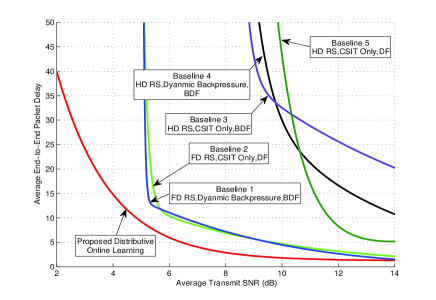
Figure 3: Average end-to-end delay versus average transmit SNR. Baseline 1 refers to the dynamic backpressure algorithm with BDF protocol and full-duplex relays. Baseline 2 refers to the CSIT only scheduling with traditional DF protocol and full-duplex relays. Baseline 3 refers to the CSIT only scheduling with BDF protocol and half-duplex relays. Baseline 4 refers to the dynamic backpressure algorithm with BDF protocol and half-duplex relays. Baseline 5 refers to the CSIT only scheduling with traditional DF protocol and half-duplex relays. The deterministic packet size is $N_{b}=25$K bits and the number of antennas at each RS is $N_{R}=4$. The packet drop rates of the Baselines 1-5 and the proposed distributive online learning are 0.2% 0.2% 13%, 3%, 24% and 0.2% respectively.

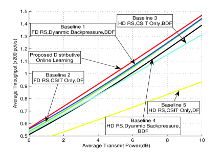
Figure 4: Average throughput versus average transmit SNR. The deterministic packet size is $N_{b}=30$K bits and the number of antennas at each RS is $N_{R}=4$. The packet drop rates of the Baselines 1-5 and the proposed distributive online learning are all 10%.

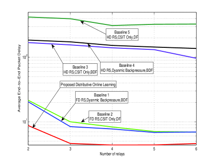
Figure 5: Average end-to-end delay versus the number of relays with transmit SNR = $5.5dB$. The deterministic packet size is $N_{b}=25$K bits and the number of antennas at each RS is $N_{R}=4$. The packet drop rates of the Baseline 1-5 and the proposed distributive online learning are 23%, 23%, 86%, 82%, 96% and 0.5% respectively.

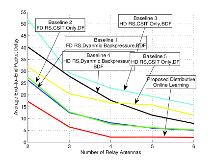
Figure 6: Average end-to-end delay versus the number of relay antennas with transmit SNR = $5dB$. The deterministic packet size is $N_{b}=20$K bits and the number of antennas at each RS is $N_{R}=4$. The packet drop rates of the Baseline 1-5 and the proposed distributive online learning are 3%, 4%, 9%, 5%, 20% and 0.1%, respectively.

In this section, we shall compare our proposed online per-node value function learning algorithm to five reference baselines. Baseline 1 and 4 refer to the proposed buffered decode and forward (BDF) protocol with throughput optimal policy (in stability sense), namely the dynamic backpressure algorithm [24], where we utilize full-duplex RSs in Baseline 1 and half-duplex RSs in Baseline 4. Baseline 2 and 5 refer to the regular decode-and-forward protocol (DF) with the CSIT only scheduling (the link selection and power allocation are adaptive to the CSIT only so as to optimize the end-to-end throughput). We utilize full-duplex RSs in Baseline 2 and half-duplex RSs in Baseline 5. Moreover, Baseline 3 refers to the proposed BDF protocol with CSIT only scheduling and half-duplex RSs. In the simulations, we assume the total bandwidth is 1 MHz, the packet arrival at the source node is Poisson with average arrival rate $\lambda_{S}=200$pck/s and deterministic packet size $N_{b}$ bits. The number of antennas at the source node and the destination node is $N_{T}=2$. Moreover, the maximum buffer size of each node (source node and RSs) is $N_{Q}=10$.

Figure 3 and Figure 4 illustrate the average end-to-end delay and average throughput versus average transmit SNR per node with $N_{R}=4$ antennas at each RS, respectively. It can be observed that the proposed distributive algorithm with half-duplex RS could achieve significant performance gain in both average delay and average throughput over all baselines with full-duplex RSs, and even more significant gain over the baselines with half-duplex RSs. This illustrates the advantages of the proposed BDF algorithm with distributive delay-optimal control policy, which could effectively reduce the intrinsic half-duplex penalty in the cooperative communication systems.

Figure 5 and Figure 6 illustrate the average end-to-end delay versus the number of relays and the number of relay antennas with $N_{R}=4$ antennas at each RS, respectively. It can be observed that the average delay of all the schemes decreases as the number of relays or the number of relay antennas increases. Furthermore, the proposed BDF algorithm with distributive delay-optimal control policy has significant gain in delay over all the baselines.

Figure 7 illustrates the convergence property of the proposed distributive online learning algorithm. We plot the per-node value function of the first relay versus scheduling slot index at a transmit SNR= $10$dB. The average delay at the $200$-th scheduling slot is already very close to the steady-state value, which is much better than all the baselines. Furthermore, unlike the iterations in deterministic NUM problems, the proposed algorithm is online, meaning that normal payload is delivered during the iteration steps.

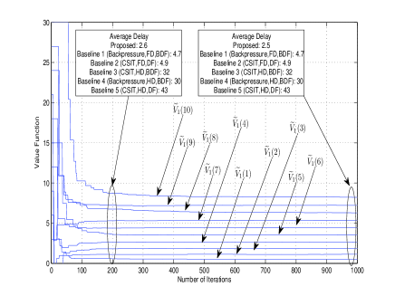
Figure 7: Illustration of the convergence of the proposed online learning algorithm. The instantaneous per-node value function is plotted versus time slot index for a cooperative MIMO system with a source node (with 2 antennas) and 2 RS nodes (each with 4 antennas). The transmit SNR of the source and the RS nodes are 10 dB and the target packet drop rate is 0.2%. Unlike the iterations in deterministic NUM problems, the proposed algorithm is online, meaning that normal payload is delivered during the iteration steps.

VI Summary

In this paper, we consider queue-aware resource control for two-hop cooperative MIMO systems. We show that by exploiting buffering in each MIMO relay, we could substantially reduce the intrinsic half-duplex loss in cooperative systems. The delay-optimal resource control policy is formulated as an average-cost infinite horizon Markov Decision Process (MDP). To obtain a low complexity solution, we approximate the value function by a linear combination of per-node value functions. The per-node value function is obtained using a distributive stochastic learning algorithm. We also established technical conditions for almost-sure convergence and show that in heavy traffic limit, the proposed low complexity distributive algorithm converges to global optimal solution.

Appendix A: Proof of Lemma 10

The average number of bits received by the source node is given by $\lambda_{S}(1-D)$, which is also the average number of information bits received by the relay clusters as the source node and the relay cluster are cascade. Let $W$, $W_{S}$ and $W_{R}$ be the average time (with the unit of frames) one information bit staying in the system, the source node’s queue and some relay’s queue respectively, $N_{S}$ and $N_{R}$ be the average number of information bits in the source node’s queue and the relays’ queues respectively, we have $N_{S}=(1-D)\lambda_{S}W_{S}$ and $N_{R}=(1-D)\lambda_{S}W_{R}$ by Little’s Law. Notice that $W=W_{S}+W_{R}$, we have $W=\frac{N_{S}+N_{R}}{\lambda_{S}(1-D)}$. Since the change of system queue state forms a Markov chain, we have $W=\mathbf{E}_{\pi_{\kappa}}\Big{[}\frac{Q_{S}+\sum_{m=1}^{M}Q_{m}}{\lambda_{S}(1-D)}\Big{]}$, where $\pi_{\kappa}$ is the steady state distribution. For sufficiently small packet drop rate requirement $1-D\approx 1$, the end to end average delay becomes $W=\mathbf{E}_{\pi_{\kappa}}\Big{[}\frac{Q_{S}+\sum_{m=1}^{M}Q_{m}}{\lambda_{S}}\Big{]}$.

Appendix B: Proof of Lemma 2

From the Bellman equation of the original state space (18), we have

$$\theta+V(\mathbf{Q}^{i},\mathbf{H})= \min_{\Pi(\mathbf{Q}^{i},\mathbf{H})}\Big{\{}g\big{(}(\mathbf{Q}^{i},\mathbf{H}),\Pi(\mathbf{Q}^{i},\mathbf{H}),\gamma\big{)}+\sum_{(\mathbf{Q}^{j},\mathbf{H}^{\prime})}\Pr\big{[}(\mathbf{Q}^{j},\mathbf{H}^{\prime})|(\mathbf{Q}^{i},\mathbf{H}),\Pi(\mathbf{Q}^{i},\mathbf{H})\big{]}J(\mathbf{Q}^{j},\mathbf{H}^{\prime})\Big{\}}$$

$$\mathrel{\mathop{=}\limits^{(a)}} \min_{\Pi(\mathbf{Q}^{i},\mathbf{H})}\Big{\{}g\big{(}(\mathbf{Q}^{i},\mathbf{H}),\Pi(\mathbf{Q}^{i},\mathbf{H}),\gamma\big{)}+\sum_{\mathbf{Q}^{j}}\Pr\big{[}\mathbf{Q}^{j}|(\mathbf{Q}^{i},\mathbf{H}),\Pi(\mathbf{Q}^{i},\mathbf{H})\big{]}V(\mathbf{Q}^{j})\Big{\}},$$ (37)

where (a) is due to the definition $V(\mathbf{Q}^{j})=\mathbf{E}_{\mathbf{H}^{\prime}}[V(\mathbf{Q}^{j},\mathbf{H}^{\prime})|\mathbf{Q}^{j}]$, and the optimal control actions are given by $\Pi^{*}(\mathbf{Q}^{i},\mathbf{H})=\arg\min_{\Pi(\mathbf{Q}^{i},\mathbf{H})}\Big{\{}g\big{(}(\mathbf{Q}^{i},\mathbf{H}),\Pi(\mathbf{Q}^{i},\mathbf{H}),\gamma\big{)}+\sum_{\mathbf{Q}^{j}}\Pr\big{[}\mathbf{Q}^{j}|(\mathbf{Q}^{i},\mathbf{H}),\Pi(\mathbf{Q}^{i},\mathbf{H})\big{]}V(\mathbf{Q}^{j})\Big{\}}$. Thus, by the partitioning of the optimal control actions in Definition 1, i.e. $\Pi^{*}(\mathbf{Q}^{i})=\{\Pi^{*}(\mathbf{Q}^{i},\mathbf{H})|\forall\mathbf{H}\}$,

$$\Pi^{*}(\mathbf{Q}^{i})=\arg\min_{\Pi(\mathbf{Q}^{i})}\sum_{\mathbf{H}}\Pr(\mathbf{H})\Big{\{}g\big{(}(\mathbf{Q}^{i},\mathbf{H}),\Pi(\mathbf{Q}^{i},\mathbf{H}),\gamma\big{)}+\sum_{\mathbf{Q}^{j}}\Pr\big{[}\mathbf{Q}^{j}|(\mathbf{Q}^{i},\mathbf{H}),\Pi(\mathbf{Q}^{i},\mathbf{H})\big{]}V(\mathbf{Q}^{j})\Big{\}}$$ (38)

From (37) and (38), we have $\theta+\Pr(\mathbf{H})V(\mathbf{Q}^{i},\mathbf{H})=\min_{\Pi(\mathbf{Q}^{i})}\sum_{\mathbf{H}}\Pr(\mathbf{H})\Big{\{}g\big{(}(\mathbf{Q}^{i},\mathbf{H}),\Pi(\mathbf{Q}^{i},\mathbf{H}),\gamma\big{)}+\sum_{\mathbf{Q}^{j}}\Pr\big{[}\mathbf{Q}^{j}|(\mathbf{Q}^{i},\mathbf{H}),\Pi(\mathbf{Q}^{i},\mathbf{H})\big{]}V(\mathbf{Q}^{j})\Big{\}}\mathrel{\mathop{=}\limits^{(b)}}\min_{\Pi(\mathbf{Q}^{i})}\Big{\{}\overline{g}\big{(}\mathbf{Q}^{i},\Pi(\mathbf{Q}^{i}),\gamma\big{)}+\sum_{\mathbf{Q}^{j}}\Pr\big{[}\mathbf{Q}^{j}|\mathbf{Q}^{i},\Pi(\mathbf{Q}^{i})\big{]}V(\mathbf{Q}^{j})\Big{\}}$, where the equality (b) is due to the definition of $\overline{g}$ in (19). As a result, the control policy obtained by solving (18) is the same as that obtained by solving (17) and this completes the proof.

Appendix C: Proof of Lemma 3

We shall prove the general control policy first, followed by the closed-form power control derivation.

According to (25), given $N_{SR}$ and $N_{RD}$, the optimal power control is given by:

$$\min_{\{\Pi_{p}^{m}\}}\mathbf{E}_{\mathbf{H}}\Big{[}\sum_{m,{N_{SR}}}I_{S,m}^{N_{SR}}G_{S,m}(N_{SR},p_{S,m})+\sum_{n,{N_{RD}}}I_{n,D}^{N_{RD}}G_{n,D}(N_{RD},p_{n,D})\Big{]}\Big{\}}$$

$$= \mathbf{E}_{\mathbf{H}}\Big{[}\sum_{m,{N_{SR}}}I_{S,m}^{N_{SR}}\min_{p_{S,m}}G_{S,m}(N_{SR},p_{S,m})+\sum_{n,{N_{RD}}}I_{n,D}^{N_{RD}}\min_{p_{m,D}}G_{n,D}(N_{RD},p_{n,D})\Big{]}\Big{\}}$$

Therefore, $p_{S,m}^{*}(N_{SR})=\arg\min_{p_{S,m}}G_{S,m}(N_{SR},p_{S,m})$ and $p_{m,D}^{*}(N_{SR})=\arg\min_{p_{m,D}}G_{n,D}(N_{RD},p_{n,D})$. To determine the optimal Rx-RS, Tx-RS and stream allocation, the biding is divided into two stages:

• First Biding: Each RS (say the $m$-th RS) broadcasts one bid for each possible $N_{SR}$ indicating that if itself is selected as Rx-RS and the number of S-R streams is $N_{SR}$, what would be the corresponding $G_{S,m}(N_{SR},p_{S,m}^{*})$.

• Second Biding: After receiving the bids in the first round, each RS (say the $n$-th RS) should calculate that if itself is selected as the Tx-RS, which RS else is the best Rx-RS (say the $m$-th RS is the best Rx-RS), what’s the best $N_{SR}$ and $N_{RD}$ and what’s the corresponding $B_{n}^{*}=G_{S,m}(N_{SR},p_{S,m}^{*})+G_{n,D}(N_{RD},p_{n,D}^{*})$. Then, broadcast the calculation results $B_{n}^{*}$ as the second bid.

• After comparing the $B_{n}^{*}$, the optimal Rx-RS, Tx-RS and stream allocation can be determined.

Therefore, the first-stage bidding and the second-stage bidding is straight-forward.

When $\lambda_{S}$ and $\frac{N_{Q}}{\lambda}$ ($m=S,1,2,...,M$) are sufficiently large, it with large probability that $\frac{Q_{m}}{\lambda}$ ($m=S,1,2,...,M$) is sufficiently large. Hence, following a similar approach in [25], it can be proved that the value function $\widetilde{V}_{m}$ ($m=S,1,2,...,M$) is increasing polynomially in $Q=[Q_{S},Q_{1},...,Q_{M}]^{T}$. The optimization on $p_{S,m}$ is given by

$$p_{S,m}^{*}(N_{SR})=\arg\min_{p_{S,m}}G_{S,m}(N_{SR},p_{S,m})$$

$$= \arg\min_{p_{S,m}}\bigg{\{}\gamma_{S,p}p_{S,m}+\sum_{n}f_{X}(n)\Big{(}\widetilde{V}_{S}\big{(}Q_{S}^{i}-R_{S,m}(N_{SR},p_{S,m})+n\big{)}-\widetilde{V}_{S}(Q_{S}^{i}+n)\Big{)}$$

$$+\widetilde{V}_{m}\big{(}Q_{m}^{i}+R_{S,m}(N_{SR},p_{S,m})\big{)}-\widetilde{V}_{m}\big{(}Q_{m}^{i}\big{)}\bigg{\}}.$$ (39)

Similar to [25], we can do Taylor expansion as follows:

$$\widetilde{V}_{S}\big{(}Q_{S}^{i}-R_{S,m}(N_{SR},p_{S,m})+n\big{)}=\widetilde{V}_{S}\big{(}Q_{S}^{i}\big{)}+\bigg{(}n-R_{S,m}(N_{SR},p_{S,m})\bigg{)}\widetilde{V}_{S}^{{}^{\prime}}\big{(}Q_{S}^{i}\big{)},$$ (40)

$$\widetilde{V}_{S}(Q_{S}^{i}+n)=\widetilde{V}_{S}\big{(}Q_{S}^{i}\big{)}+n\widetilde{V}_{S}^{{}^{\prime}}\big{(}Q_{S}^{i}\big{)}$$ (41)

where $\widetilde{V}_{S}^{{}^{\prime}}$ is the first order derivative on $\widetilde{V}_{S}$ and the higher order is neglectable. Same apporach can be used to expand $\widetilde{V}_{m}\big{(}Q_{m}^{i}+R_{S,m}(N_{SR},p_{S,m})\big{)}$ as $\widetilde{V}_{m}\big{(}Q_{m}^{i}+R_{S,m}(N_{SR},p_{S,m})\big{)}=\widetilde{V}_{m}\big{(}Q_{m}^{i}\big{)}+R_{S,m}(N_{SR},p_{S,m})\widetilde{V}_{m}^{{}^{\prime}}\big{(}Q_{m}^{i}\big{)}$. At high SNR region, we have

$$\frac{\partial R_{S,m}(N_{SR},p_{S,m})}{\partial p_{S,m}}=\frac{N}{\ln 2}\frac{1}{p_{S,m}+\sum_{j=1}^{N_{SR}}\frac{1}{\eta_{S,m}^{j}}}.$$ (42)

According to (40,41,42), taking derivative on the RHS of (39) and letting it be zero, we can get the closed-from expression for power allocation in (29). Moreover, (30) can be proved in the same way. Finally, when $Q_{m}$ and $Q_{S}$ are sufficiently large, according to the definition of derivative, we have

$$\widetilde{V}_{S}^{{}^{\prime}}(Q_{S}^{i})=\frac{\widetilde{V}_{S}(Q_{S}^{i}+1)-\widetilde{V}_{S}(Q_{S}^{i}-1)}{2}\qquad\widetilde{V}_{m}^{{}^{\prime}}(Q_{m}^{i})=\frac{\widetilde{V}_{m}(Q_{m}^{i}+1)-\widetilde{V}_{m}(Q_{m}^{i}-1)}{2}.$$

Appendix D: Proof of Lemma 4

From [26], the convergence property of the asynchronous update and synchronous update is the same. Therefore, we consider the convergence of related synchronous version without loss of generality.

Let $c\in R$ be a constant, we have $T_{I}(c\widetilde{V}_{S}^{l})=cT_{I}(\widetilde{V}_{S}^{l})$, where $T_{I}$ is one element of mapping $\mathbf{T}$ corresponding to the state with all buffers empty. Similar to [27], the per-node value function $\{\widetilde{\mathbf{V}}_{m}\}$ is bounded almost surely during the iterations of algorithm. According to the construction of parameter vector $\mathbf{W}$, the update on $\widetilde{\mathbf{V}}_{m}$ is equivalent to the update on $\mathbf{W}$ and proving the convergence of Lemma 4 is equivalent to proving the convergence of update on $\mathbf{W}$. In the following, we first introduce and prove the following lemma on the convergence of learning noise.

Lemma 6

Define $\mathbf{q}^{l}=\mathbf{M}^{{\dagger}}\Big{[}\overline{\mathbf{g}}(\Pi_{l})+\mathbf{P}(\Pi_{l})\mathbf{M}\mathbf{W}^{l}-\mathbf{M}\mathbf{W}^{l}-T_{I}(\mathbf{M}\mathbf{W}^{l})\mathbf{e}\Big{]}$, when the number of iterations $l\geq j\rightarrow\infty$, the procedure of update can be written as follows with probability 1: $\mathbf{W}^{l+1}=\mathbf{W}^{j}+\sum_{i=j}^{l}\epsilon_{v}^{i}\mathbf{q}_{m}^{i}$.

The proof of above lemma follows the standard approach of stochastic approximation with Martingale noise [22]. Moreover, the following lemma is about the limit of sequence $\{\mathbf{q}_{m}^{l}\}$.

Lemma 7

Suppose the following two inequalities are true for $l=a,a+1,...,a+b$

$$\overline{\mathbf{g}}(\Pi^{l})+\mathbf{P}(\Pi^{l})\mathbf{M}\mathbf{W}^{l}\leq \overline{\mathbf{g}}(\Pi^{l-1})+\mathbf{P}(\Pi^{l-1})\mathbf{M}\mathbf{W}^{l}$$ (43)

$$\overline{\mathbf{g}}(\Pi^{l-1})+\mathbf{P}(\Pi^{l-1})\mathbf{M}\mathbf{W}^{l-1}\leq \overline{\mathbf{g}}(\Pi^{l})+\mathbf{P}(\Pi^{l})\mathbf{M}\mathbf{W}^{l-1},$$ (44)

then we have

$$|q^{a+b}_{i}|\leq C_{1}\prod_{i=0}^{\lfloor\frac{b}{\beta}\rfloor-1}(1-\tau^{a+i\beta})\quad\forall i,$$ (45)

where $q_{i}^{a+b}$ denotes the $i$th element of the vector $\mathbf{q}^{a+b}$, $C_{1}$ is some constant.

Proof:

From (43) and (44), we have

$$\mathbf{q}^{l}=\mathbf{M}^{{\dagger}}\big{[}\overline{\mathbf{g}}(\Pi^{l})+\mathbf{P}(\Pi^{l})\mathbf{M}\mathbf{W}^{l}-\mathbf{M}\mathbf{W}^{l}-w_{l}\mathbf{e}\big{]}\leq\mathbf{M}^{{\dagger}}\big{[}\overline{\mathbf{g}}(\Pi^{l-1})+\mathbf{P}(\Pi^{l-1})\mathbf{M}\mathbf{W}^{l}-\mathbf{M}\mathbf{W}^{l}-w_{l}\mathbf{e}\big{]}$$

$$\mathbf{q}^{l-1}= \mathbf{M}^{{\dagger}}\big{[}\overline{\mathbf{g}}(\Pi^{l-1})+\mathbf{P}(\Pi^{l-1})\mathbf{M}\mathbf{W}^{l-1}-\mathbf{M}\mathbf{W}^{l-1}-w_{l-1}\mathbf{e}\big{]}$$

$$\leq \mathbf{M}^{{\dagger}}\big{[}\overline{\mathbf{g}}(\Pi^{l})+\mathbf{P}(\Pi^{l})\mathbf{M}\mathbf{W}^{l-1}-\mathbf{M}\mathbf{W}^{l-1}-w_{l-1}\mathbf{e}\big{]}$$

where $w_{l}=T_{I}(\mathbf{M}\mathbf{W}^{l})=T_{I}(\mathbf{M}\mathbf{W}^{l})$. According to Lemma 6, we have $\mathbf{W}^{l}=\mathbf{W}^{l-1}+\epsilon_{v}^{l-1}\mathbf{q}^{l-1}\Rightarrow\mathbf{W}^{l}=\mathbf{W}^{l-1}+\epsilon_{v}^{l-1}\mathbf{q}^{l-1}$. Therefore,

$$\mathbf{q}^{l}\leq \big{[}(1-\epsilon_{v}^{l-1})\mathbf{I}+\mathbf{M}^{{\dagger}}\mathbf{P}(\Pi^{l-1})\mathbf{M}\epsilon_{v}^{l-1}\big{]}\mathbf{q}^{l-1}+w_{l-1}\mathbf{e}-w_{l}\mathbf{e}=\mathbf{B}^{l-1}\mathbf{q}^{l-1}+w_{l-1}\mathbf{e}-w_{l}\mathbf{e}$$

$$\mathbf{q}^{l}\geq \big{[}(1-\epsilon_{v}^{l-1})\mathbf{I}+\mathbf{M}^{{\dagger}}\mathbf{P}(\Pi^{l})\mathbf{M}\epsilon_{v}^{l-1}\big{]}\mathbf{q}^{l-1}+w_{l-1}\mathbf{e}-w_{l}\mathbf{e}=\mathbf{A}^{l-1}\mathbf{q}^{l-1}+w_{l-1}\mathbf{e}-w_{l}\mathbf{e}.$$

Notice that $\mathbf{A}^{l-1}\mathbf{e}=\mathbf{B}^{l-1}\mathbf{e}$, we have $\mathbf{A}^{l-1}...\mathbf{A}^{l-\beta}\mathbf{q}^{l-\beta}-C_{1}\mathbf{e}\leq\mathbf{q}^{l}\leq\mathbf{B}^{l-1}...\mathbf{B}^{l-\beta}\mathbf{q}^{l-\beta}-C_{1}\mathbf{e}$

$$\Rightarrow (1-\tau^{l})[\min\mathbf{q}^{l-\beta}]\leq\mathbf{q}^{l}+C_{1}\mathbf{e}\leq(1-\tau^{l})[\max\mathbf{q}^{l-\beta}]\Rightarrow\begin{cases}\max\mathbf{q}^{l}+C_{1}\leq(1-\tau^{l})\max\mathbf{q}^{l-\beta}\\ \min\mathbf{q}^{l}+C_{1}\geq(1-\tau^{l})\min\mathbf{q}^{l-\beta}\end{cases}$$

$$\Rightarrow \max\mathbf{q}^{l}-\min\mathbf{q}^{l}\leq(1-\tau^{l})[\max\mathbf{q}^{l-\beta}-\min\mathbf{q}^{l-\beta}]\Rightarrow|q^{l}_{i}|\leq\max\mathbf{q}^{l}-\min\mathbf{q}^{l}\leq C_{2}(1-\tau^{l})\quad\forall i,$$

where the first step is due to conditions of Lemma 4 on matrix sequence $\{\mathbf{A}^{l}\}$ and $\{\mathbf{B}^{l}\}$, $\max\mathbf{q}^{l}$ and $\min\mathbf{q}^{l}$ denote the maximum and minimum elements in $\mathbf{q}^{l}$ respectively, $C_{1}$ and $C_{2}$ are all constants, the first inequality of the last step is because $\min\mathbf{q}^{l}\leq 0$. This completes the proof of Lemma 7. ∎

Therefore, the proof of Lemma 4 can be divided into the following steps: (1) From the property of sequence $\{\epsilon_{v}^{l}\}$, we have $\prod_{i=0}^{\lfloor\frac{l}{\beta}\rfloor-1}(1-\epsilon_{v}^{i\beta})\rightarrow 0$ ($l\rightarrow\infty$). (2) According to the first step, note that $\tau^{l}=\mathcal{O}(\epsilon_{v}^{l})$, from (45), we have $\mathbf{q}^{l}\rightarrow 0$ ($l\rightarrow\infty$). (3) Therefore, the update on $\{\mathbf{W}^{l}\}$ will converge, and the fixed point of the convergence $\mathbf{W}^{\infty}$ satisfies $T_{I}(\mathbf{M}\mathbf{W}^{l})\mathbf{e}+\mathbf{W}^{\infty}=\mathbf{M}^{{\dagger}}\mathbf{T}(\mathbf{M}\mathbf{W}^{\infty})$.

Appendix E: Proof of Lemma 5

Due to the page limit, we only provide the sketch of the proof. The convergence proof of the LMs $\{\gamma_{S,p},\gamma_{1,p},...,\gamma_{M,p}\}$ for a given $\gamma_{S,d}$ is as follows:

• For the notation convenience, we first define the average transmit power of each node as follows: $\widetilde{\mathcal{P}}_{S}(\gamma)=\mathbf{E}^{\Pi}\Big{[}\sum_{m=1}^{M}\sum_{i=1}^{\min(N_{T},N_{R})}\eta_{S,m}^{i}p_{S,m}^{i}\Big{]}\quad\mbox{and}\quad\widetilde{\mathcal{P}}_{m}(\gamma)=\mathbf{E}^{\Pi}\Big{[}\sum_{m=1}^{M}\sum_{i=1}^{\min(N_{T},N_{R})}\eta_{m,D}^{i}p_{m,D}^{i}\Big{]}$ ($m=1,2,...,M$), where $\mathbf{E}^{\Pi}[\cdot]$ denotes the expectation w.r.t. the policy $\Pi(\gamma)$. Using standard stochastic approximation theory, the dynamics of the LMs update equation $\{\gamma_{S,p},\gamma_{1,p},...,\gamma_{M,p}\}$ can be represented by the following ODE:

  $$\big{[}\dot{\gamma}_{S,p}(t),...,\dot{\gamma}_{M,p}(t)\big{]}^{T}=\big{[}\widetilde{\mathcal{P}}_{S}(\gamma)-P_{S},\widetilde{\mathcal{P}}_{1}(\gamma)-P_{R},...,\widetilde{\mathcal{P}}_{M}(\gamma)-P_{R}\big{]}^{T}.$$ (46)

• Using perturbation analysis in [28], we have $\frac{\partial\widetilde{\mathcal{P}}_{m}(\gamma)}{\partial\gamma_{m,p}}<0$ ($m=S,1,2,...,M$) and $\Big{|}\frac{\partial\widetilde{\mathcal{P}}_{m}(\gamma)}{\partial\gamma_{m,p}}\Big{|}>>\Big{|}\frac{\partial\widetilde{\mathcal{P}}_{m}(\gamma)}{\partial\gamma_{n,p}}\Big{|}$ ($m=S,1,2,...,M,n\neq m$). Thus, the update of $\gamma_{m,p}$ ($m=S,1,...,M$) in ODE (46) will drive $\widetilde{\mathcal{P}}_{m}-P_{R}$ (or $\widetilde{\mathcal{P}}_{S}-P_{S}$) to 0 whenever $\widetilde{\mathcal{P}}_{m}-P_{R}$ (or $\widetilde{\mathcal{P}}_{S}-P_{S}$) is non-zero. Therefore, the ODE (46) will converge. The converged LMs $\{\gamma_{S,p}^{*}(\gamma_{S,d}),\gamma_{1,p}^{*}(\gamma_{S,d}),...,\gamma_{M,p}^{*}(\gamma_{S,d})\}$ can be characterized by the equilibrium point of the ODE (46), which is given by the RHS of (46) $\rightarrow 0$.

Suppose for a given $\gamma_{S,d}$, $\{\gamma_{S,p},\gamma_{1,p},...,\gamma_{M,p}\}$ converge to $\{\gamma_{S,p}^{*}(\gamma_{S,d}),\gamma_{1,p}^{*}(\gamma_{S,d}),...,\gamma_{M,p}^{*}(\gamma_{S,d})\}$. Since $\frac{\partial\big{(}\mathbf{E}^{\Pi}_{\gamma_{1,p}^{*},...,\gamma_{M,p}^{*},\gamma_{S,p}^{*}}[Q_{S}=N_{Q}]\big{)}}{\partial\gamma_{S,d}}<0$, the update on $\gamma_{S,d}$ will converge as well for a similar reason as in the convergence of $\{\gamma_{S,p},\gamma_{1,p},...,\gamma_{M,p}\}$. Similarly, the converged $\gamma_{S,d}^{*}$ can be characterized by the equilibrium point of the ODE $\dot{\gamma}_{S,d}(t)=\mathbf{E}^{\Pi}_{\gamma_{1,p}^{*},...,\gamma_{M,p}^{*},\gamma_{S,p}^{*}}[Q_{S}=N_{Q}]-D$, which is given by the RHS $\rightarrow 0$.

Appendix F: Proof of Theorem 2

Without loss of generality, we shall consider the approximate value function $V(\mathbf{Q})=\sum_{m=S}^{M}\sum_{q=1}^{N_{Q}}\widetilde{V}_{m}(q)$ $\mathbf{I}[Q_{m}=q]$ on the following redefined set of representative states $\mathcal{Q}_{R}=\{\delta_{m,q}|m=S,1,2,...,M;q=0,1,...,q_{I}-1,q_{I}+1,...,N_{Q}\}$, where the state $\delta_{m,q}$ is given by $\delta_{m,q}=[Q_{S}=q_{I},Q_{1}=q_{I},...,Q_{m}=q,...,Q_{M}=q_{I}]^{T}$ and $q_{I}<N_{Q}$ is sufficiently large. Correspondingly, $\mathbf{M}^{-1}$ should also be redefined such that the per-node value function $\{\widetilde{\mathbf{V}}_{m}\}$ is updated on the representative states $\mathcal{Q}_{R}$ [21].

First of all, following the similar approach in the proof of Lemma 4, the per-node value function (under the new reference states) would also converge almost surely to $\{\widetilde{\mathbf{V}}_{m}^{\infty}(\gamma)\}$ for any given LMs $\gamma$.

Next, when the conditions of Theorem 2 are satisfied, given any $\epsilon>0$, there is one integer $Q_{0}(\epsilon)$ such that for all $q>Q_{0}(\epsilon)$ and $q_{I}=Q_{0}(\epsilon)$, we have (from the proof of Lemma 3):

$$\widetilde{V}_{m}^{\infty}(q-r)-\widetilde{V}_{m}^{\infty}(q)=\widetilde{V}_{m}^{\infty}(q_{I}-r)-\widetilde{V}_{m}^{\infty}(q_{I})+\mathcal{O}(\epsilon).$$ (47)

Moreover, since $\{\widetilde{V}_{m}^{\infty}(q)\}$ are all monotonically increasing functions with respect to $q$ and $\{\widetilde{V}_{m}^{\infty}(N_{Q})\}$ are all bounded, we have $\widetilde{V}_{m}\Big{(}Q_{0}(\epsilon)\Big{)}=\mathcal{O}(\epsilon)$ for sufficiently large arrivals. Therefore, (47) holds for all $q\in[0,N_{Q}]$ for sufficiently large $N_{Q}$ and input arrivals. Similarly, we have

$$\widetilde{V}_{S}^{\infty}(q+n-r)-\widetilde{V}_{S}^{\infty}(q+n)=\widetilde{V}_{S}^{\infty}(q_{I}+n-r)-\widetilde{V}_{S}^{\infty}(q_{I}+n)+\mathcal{O}(\epsilon)$$ (48)

$$\widetilde{V}_{m}^{\infty}(q+r)-\widetilde{V}_{m}^{\infty}(q)=\widetilde{V}_{m}^{\infty}(q_{I}+r)-\widetilde{V}_{m}^{\infty}(q_{I})+\mathcal{O}(\epsilon).$$ (49)

Hence, with the above equations and substituting the converged per-node value function $\{\widetilde{\mathbf{V}}_{m}^{\infty}(\gamma)\}$ into (18) for the reference states, we get

$$\widetilde{V}_{S}^{\infty}(q)= q+\gamma_{S,d}\mathbf{I}[q=N_{Q}]+\sum_{n}f_{X}(n)\Big{(}\widetilde{V}_{S}^{\infty}(q+n)-\widetilde{V}_{S}^{\infty}(n)\Big{)}+\min_{\Pi}\mathbf{E}_{\mathbf{H}}\Big{\{}\sum_{m,N_{SR}}\eta_{S,m}^{N_{SR}}\Big{[}\gamma_{S,p}\sum_{k}p_{S,m}^{N_{SR}}$$

$$+\sum_{n}f_{X}(n)\Big{(}\widetilde{V}_{S}^{\infty}(q+n-r_{S,m}^{N_{SR}})-\widetilde{V}_{S}^{\infty}(q+n)\Big{)}+\widetilde{V}_{m}^{\infty}(q_{I}+r_{S,m}^{N_{SR}})-\widetilde{V}_{m}^{\infty}(q_{I})\Big{]}\Big{\}}$$ (50)

$$\widetilde{V}_{m}^{\infty}(q)= q+\widetilde{V}_{m}^{\infty}(q)+\min_{u}\mathbf{E}_{\mathbf{H}}\Big{\{}\sum_{N_{RD}}\eta_{m,D}^{N_{RD}}\Big{[}\gamma_{m,p}\sum_{k}p_{m,D}^{N_{RD}}+\widetilde{V}_{m}^{\infty}(q-r_{m,D}^{N_{RD}})-\widetilde{V}_{m}^{\infty}(q)\Big{]}\Big{\}},$$ (51)

where $m=1,2,...,M$.

Finally, for any system state $\mathbf{Q}^{i}=[Q_{S}^{i},...,Q_{M}^{i}]^{T}$, substitute the above equations into the RHS of the original Bellman equation in (18), we get RHS of (18) $\mathrel{\mathop{=}\limits^{\rm a}}\sum_{m=S}^{M}Q_{m}^{i}+\gamma_{S,d}\mathbf{I}[Q_{S}^{i}=N_{Q}]+\sum_{n}f_{X}(n)\widetilde{V}_{S}^{\infty}(Q_{S}^{i}+n)+\sum_{m=1}^{M}\widetilde{V}_{m}^{\infty}(Q_{m}^{i})+\min_{\Pi(\mathbf{Q}^{i})}\mathbf{E}_{\mathbf{H}}\Big{\{}\sum_{m,N_{SR}}\eta^{N_{SR}}_{S,m}\Big{[}\gamma_{S,p}p_{S,m}^{N_{SR}}+\sum_{n}f_{X}(n)\Big{(}\widetilde{V}^{\infty}_{S}(Q_{S}^{i}+n-r_{S,m}^{N_{SR}})-\widetilde{V}^{\infty}_{S}(Q_{S}^{i}+n)\Big{)}+\widetilde{V}^{\infty}_{m}(q_{I}+r_{S,m}^{N_{SR}})-\widetilde{V}^{\infty}_{m}(q_{I})\Big{]}+\sum_{m,N_{RD}}\eta^{N_{RD}}_{m,D}\Big{[}\gamma_{m,p}p_{m,D}^{N_{RD}}+\widetilde{V}^{\infty}_{m}(Q_{m}^{i}-r_{m,D}^{N_{RD}})-\widetilde{V}^{\infty}_{m}(Q_{m}^{i})\Big{]}\Big{\}}+\mathcal{O}(\epsilon)\mathrel{\mathop{=}\limits^{\rm b}}\sum_{m=S}^{M}\widetilde{V}_{m}^{\infty}(Q_{m}^{i})+\sum_{n}f_{I}(n)\widetilde{V}_{S}^{\infty}(n)+\mathcal{O}(\epsilon)=V(\mathbf{Q}^{i})+\sum_{n}f_{I}(n)\widetilde{V}_{S}^{\infty}(n)+\mathcal{O}(\epsilon)$, where equality (a) is due to (49), equality (b) is due to (50) and (51). Since $\sum_{n}f_{X}(n)\widetilde{V}_{S}^{\infty}(n)$ is a constant independent of $\mathbf{Q}^{i}$ and $\epsilon$ is chosen arbitrarily, we have shown that the approximate value function $V(\mathbf{Q})=\sum_{m=S}^{M}\sum_{q=1}^{N_{Q}}\widetilde{V}^{\infty}_{m}(q)\mathbf{I}[Q_{m}=q]$ can satisfy the original Bellman equation (18) asymptotically (when $N_{Q}\rightarrow+\infty$). As a result, the proposed distributive update algorithm converges to the global optimal solution and this completes the proof.

References

- [1] E. van der Meulen, “Transmission of information in a t-terminal discrete memoryless channel,” Ph.D. dissertation, Dep. of Statistics, University of California, Berkeley, 1968.
- [2] T. Cover and A. Gamal, “Capacity theorems for the relay channel,” IEEE Transactions on Information Theory, vol. 25, no. 5, pp. 572–584, Sep 1979.
- [3] IEEE 802.16’s Relay Task Group. [Online]. Available: http://www.ieee802.org/16/relay/index.html.
- [4] WINNER- Wireless World Initiative New Radio. [Online]. Available: http://www.ist-winner.org/.
- [5] P. Yip and D. Etter, “An adaptive technique for multiple echo cancelation in telephone networks,” in Acoustics, Speech, and Signal Processing, IEEE International Conference on ICASSP ’87., vol. 12, Apr 1987, pp. 2133–2136.
- [6] L. Vega, H. Rey, J. Benesty, and S. Tressens, “A new robust variable step-size nlms algorithm,” IEEE Transactions on Signal Processing, vol. 56, no. 5, pp. 1878–1893, May 2008.
- [7] E. Lo and K. Letaief, “Optimizing downlink throughput with user cooperation and scheduling in adaptive cellular networks,” in Wireless Communications and Networking Conference, 2007.WCNC 2007. IEEE, March 2007, pp. 4342–4347.
- [8] D. P. Bertsekas, Dynamic Programming - Deterministic and Stochastic Models. Prentice Hall, NJ, USA, 1987.
- [9] X. Cao, Stochastic Learning and Optimization: A Sensitivity-Based Approach. Springer, 2008.
- [10] E. Yeh and R. Berry, “Throughput optimal control of cooperative relay networks,” in Information Theory, 2005. ISIT 2005. Proceedings. International Symposium on, Sept. 2005, pp. 1206–1210.
- [11] L. Georgiadis, M. J. Neely, and L. Tassiulas, “Resource allocation and cross-layer control in wireless networks,” Foundations and Trends in Networking, vol. 1, no. 1, pp. 1–144, 2006.
- [12] J. Abounadi, D. Bertsekas, and V. S. Borkar, “Learning algorithms for markov decision processes with average cost,” SIAM Journal on Control and Optimization, vol. 40, pp. 681–698, 1998.
- [13] T. Richardson and R. Urbanke, “The capacity of low-density parity-check codes under message-passing decoding,” IEEE Transactions on Information Theory, vol. 47, no. 2, pp. 599–618, Feb 2001.
- [14] S. Boyd and L. Vandenberghe, Convex Optimization. Cambridge University Press, 2004.
- [15] Z. Han, Z. Ji, and K. Liu, “Non-cooperative resource competition game by virtual referee in multi-cell ofdma networks,” IEEE Journal on Selected Areas in Communications, vol. 25, no. 6, pp. 1079–1090, August 2007.
- [16] D. Palomar and M. Chiang, “Alternative distributed algorithms for network utility maximization: Framework and applications,” IEEE Transactions on Automatic Control, vol. 52, no. 12, pp. 2254–2269, Dec. 2007.
- [17] J. Huang, R. Berry, and M. L. Honig, “Auction-based spectrum sharing,” ACM Mobile Networks and Applications Journal (MONET), vol. 11, pp. 405–418, June 2006.
- [18] C. Curescu and S. Nadjm-Tehrani, “A bidding algorithm for optimized utility-based resource allocation in ad hoc networks,” IEEE Transactions on Mobile Computing, vol. 7, no. 12, pp. 1397–1414, Dec. 2008.
- [19] D. Bertsekas, Dynamic Programming and Optimal Control, Vol. 2. Athena Scientific, 2007.
- [20] V.S.Borkar, “An actor-critic algorithm for constrained markov decision processes,” in Systems Control Lett. 54, 2005, pp. 207–213.
- [21] J. N. Tsitsiklis and B. van Roy, “Feature-based methods for large scale dynamic programming,” Machine Learning, vol. 22, pp. 59–94, March 1996.
- [22] V. S. Borkar, Stochastic Approximation: A Dynamical Systems Viewpoint. Cambridge University Press, 2008.
- [23] ——, “Stochastic approximation with two time scales,” Systems Control Lett. 29, pp. 291–294, 1997.
- [24] L. Georgiadis, M. Neely, and L. Tassiulas, Resource Allocation and Cross Layer Control in Wireless Networks. Now Publishers Inc, 2006.
- [25] I. Bettesh and S. Shamai, “Optimal power and rate control for minimal average delay: The single-user case,” IEEE Transactions on Information Theory, vol. 52, no. 9, pp. 4115–4141, Sept. 2006.
- [26] V. S. Borkar, “Asynchronous stochastic approximation,” SIAM J. Control and Optim., vol. 36, pp. 840–851, 1998.
- [27] V. S. Borkar and S. P. Meyn, “The ode method for convergence of stochastic approximation and reinforcement learning algorithms,” SSIAM J. on Control and Optimization 38, pp. 447–469, 2000.
- [28] X. Cao, Stochastic Learning and Optimization: A Sensitivity-Based Approach. Springer, 2007.