Efficient tomography of quantum processes

Abstract

We show with explicit formulas that one can completely identify an unknown quantum process with only one weakly entangled state; and identify a quantum optical Gaussian process with either one two-mode squeezed state or a few different coherent states. In tomography of a multi-mode process, our method reduces the number of different test states exponentially compared with existing methods.

Introduction.— One of the basic problems of quantum physics is to predict the evolution of a quantum system under certain conditions. For an isolated system with a known Hamiltonian, the evolution is characterized by a unitary operator determined by the Schrödinger equation. However, the system may interact with its environment, and the total Hamiltonian of the system plus the environment is in general not completely known. The evolution can then be regarded as a “black-box process” qpt which maps the input state into an output state. An important problem here is how to characterize an unknown process by testing the black-box with some specific input states, i.e., quantum process tomography (QPT) qpt .

Any physical process can be described by a completely positive map $\varepsilon$. Such a process is fully characterized if the evolution of any input state $\rho_{\rm in}$ is predictable: $\rho_{\rm out}=\varepsilon(\rho_{\rm in})$. In general, QPT is very difficult to implement in high dimensional spaces, and, more challengingly, in an infinite dimensional space, such as a Fock space. Recently, Ref. calgary showed QPT in Fock space, for Continuous Variable (CV) states. Two conclusions calgary are: ($i$) If the output states of all coherent input states are known, then one can predict the output state of any input state; ($ii$) By taking the “photon-number-cut-off approximation”, one can then characterize an unknown process with a finite number of different input coherent states (CSs).

Here we study QPT using a different approach. Based on the idea of isomorphism liusky , and using the standard $Q$-representation in quantum optics, we show, with explicit formulas, that one can complete QPT with either only one weakly entangled state for any quantum process, or only a few CSs for quantum optical Gaussian processes. The method described here has several advantages. First, it presents explicit formulas without any approximation, such as the photon-number-cut-off approximation. Second, it requires only one or a few different states to characterize a process, rather than all CSs. Third, for multi-mode Gaussian process tomography, the number of input CSs increases polynomially with the number of modes, rather than exponentially. Fourth, it uses $Q$-functions only, which is always well-defined for any state without any higher order singularities in the calculation.

Isomorphism and process tomography with one weakly entangled state.— Define $|\Phi^{+}\rangle=\sum_{k=0}^{s-1}|kk\rangle$ as the $s$-level maximally entangled state in the composite space of modes $a$ and $b$. (Here $|\Phi^{+}\rangle$ is not normalized, because this simplifies the calculations below). Assume now that the process $\varepsilon$ acts on mode $b$. Using isomorphism liusky , if the state $\rho_{\varepsilon}=I\otimes\varepsilon(|\Phi^{+}\rangle\langle\Phi^{+}|)$ is known, we shall know $\varepsilon(\rho_{{\rm in}})$ for any single-mode input state $\rho_{{\rm in}}$ on mode $b$. Consider a single-mode input state on mode $b$, $|\psi(\{c_{k}\})\rangle=\sum_{k}c_{k}|k\rangle$. Obviously it can be written as

$$\left(|\psi\rangle\langle\psi|\right)_{b}={{}_{a}}\langle\psi^{*}|\Phi^{+}\rangle\langle\Phi^{+}|\psi^{*}\rangle_{a}$$

$$={\rm tr_{a}}\left(|\psi^{*}\rangle\langle\psi^{*}|\otimes I\cdot|\Phi^{+}\rangle\langle\Phi^{+}|\right)$$ (1)

and $|\psi^{*}\rangle_{a}=\sum_{k}c_{k}^{*}|k\rangle_{a}$, is a single-mode state on mode $a$ (sometimes we omit the subscript $a$ or $b$ for simplicity). The output for any initial state $\rho_{{\rm in}}=\left(|\psi\rangle\langle\psi|\right)_{b}$ is

$$\rho_{{\rm out}}=\varepsilon\left\{{\rm tr_{a}}\left[\left(|\psi^{*}\rangle\langle\psi^{*}|\right)\!_{a}\otimes I_{b}\cdot\left(|\Phi^{+}\rangle\langle\Phi^{+}|\right)\!_{ab}\right]\right\}$$ (2)

Since the partial trace and the map $\varepsilon$ are taken in different subspaces, their orders can be exchanged. Thus

$$\rho_{{\rm out}}={{}_{a}\langle}\psi^{*}|I\otimes\varepsilon(|\Phi^{+}\rangle\langle\Phi^{+}|)|\psi^{*}\rangle_{a}={{}_{a}\langle}\psi^{*}|\rho_{\varepsilon}|\psi^{*}\rangle_{a}$$

$$={\rm tr_{a}}\left(|\psi^{*}\rangle\langle\psi^{*}|\otimes I\cdot\rho_{\varepsilon}\right).$$ (3)

Equation (Efficient tomography of quantum processes) predicts the output state of any input state of an unknown process, given $\rho_{\varepsilon}$. However, generating the maximum entangled state $|\Phi^{+}\rangle$ is technologically difficult, especially when $s$ is large. Moreover, for the case of CV states in Fock space, $s$ is infinite and the maximum entanglement does not physically exist. Therefore, we cannot really test a process with $|\Phi^{+}\rangle$ in Fock space. However, we can first test a process with some other easy-to-manipulate states, and then deduce the state $\rho_{\varepsilon}$. For example, one can test the one-sided map $I\otimes\varepsilon$ with an arbitrary non-maximally entangled state $|\phi(\{r_{k}\})\rangle=\sum_{k=0}^{s-1}r_{k}|kk\rangle$, if $r_{0}\cdot r_{1}\cdots r_{s-1}\not=0$. Denoting the output state as $\Omega_{\{r_{k}\}}$, we have

$$\Omega_{\{r_{k}\}}=I\otimes\varepsilon(|\phi(\{r_{k}\})\langle\phi(\{r_{k}\})|).$$ (4)

On the other hand, we know that $|\phi(r_{k})\rangle=\hat{T}(\{r_{k}\})\otimes I|\Phi^{+}\rangle$; and $\hat{T}(\{r_{k}\})$ is a projection operator defined as $\hat{T}(\{r_{k}\})=\sum_{k=0}^{s-1}r_{k}|k\rangle\langle k|$. Since $\hat{T}\otimes I$ and the one-sided map $I\otimes\varepsilon$ commute, then Eq. (4) can be written as

$$\Omega_{\{r_{k}\}}=\hat{T}(\{r_{k}\})\otimes I\left\{I\otimes\varepsilon\left[|\Phi^{+}\rangle\langle\Phi^{+}\right]\right\}\hat{T}(\{r_{k}\})\otimes I$$ (5)

which gives rise to

$$\rho_{\varepsilon}=\hat{T}^{-1}(\{r_{k}\})\otimes I\,\Omega_{\{r_{k}\}}\,\hat{T}^{-1}(\{r_{k}\})\otimes I.$$ (6)

Here $\hat{T}^{-1}(\{r_{k}\})$ is defined as $\hat{T}(\{r_{k}^{-1}\})$. If we test the one-sided map $I\otimes\varepsilon$ with the limited entangled state $|\phi(\{r_{k}\})\rangle$ and we find that the outcome state is $\Omega_{\{r_{k}\}}$, then, using Eq. (6) we can determine the output state when the input state is $|\Phi^{+}\rangle$. We can then use Eq. (Efficient tomography of quantum processes) to predict the output state of any single-mode input state on mode $b$. Explicitly, if the input state is $|\psi(\{c_{k}\})\rangle=\sum_{k}c_{k}|k\rangle$, the output state becomes

$$\rho_{\psi}={\rm tr_{a}}\left[|\psi({c_{k}^{*}}/{r_{k}})\rangle\langle\psi({c_{k}^{*}}/{r_{k}})|\otimes I\cdot\Omega_{\{r_{k}\}}\right]$$ (7)

where $|\psi({c_{k}^{*}}/{r_{k}})\rangle=\sum_{k}({c_{k}^{*}}/{r_{k}})|k\rangle$.

For a state in Fock space, $s$ is infinite and $|k\rangle$ is a Fock state which can be generated by the creation operator $a^{\dagger}$ on the vacuum state $|0\rangle$. We can implement a similar technique to the one presented above to characterize an unknown quantum optical process with only one weakly-entangled state, i.e., a two-mode squeezed state (TMSS).

Process tomography with one TMSS.— A TMSS is defined by $|\chi(q)\rangle=c_{q}\exp({qa^{\dagger}b^{\dagger}})|00\rangle$, where $c_{q}=\sqrt{1-q^{2}}$, and $q$ is real. The (un-normalized) maximally-entangled state here is $|\Phi^{+}\rangle=\lim_{q\rightarrow 1}\exp(qa^{\dagger}b^{\dagger})|00\rangle=\sum_{k=0}^{\infty}|kk\rangle$, where $x^{\dagger}$ is the creation operator for mode $x$.

We define the projection operator $\hat{T}(q)=c_{q}\exp[(\ln q)a^{\dagger}a]$ which has the property: $\hat{T}(q)\;(a,a^{\dagger})\;\hat{T}^{-1}(q)=(a/q,qa^{\dagger})$. The TMSS $|\chi(q)\rangle$ can be written as

$$|\chi(q)\rangle=\hat{T}(q)\otimes I|\Phi^{+}\rangle.$$ (8)

Assume now that the black box process acts only on mode $b$ of the bipartite state $|\chi(q)\rangle$. After the process, we obtain a two-mode state $\Omega_{q}$. We now wish to predict the evolution of any state under the same process, using the information on how the input state $|\chi(q)\rangle$ changes under this map. According to Eq. (8), we have

$$\Omega_{q}=\hat{T}(q)\otimes I\cdot\rho_{\varepsilon}\cdot\hat{T}(q)\otimes I$$ (9)

where $\rho_{\varepsilon}=I\otimes\varepsilon\left(|\Phi^{+}\rangle\langle\Phi^{+}|\right)$. Naturally,

$$\rho_{\varepsilon}=\hat{T}^{-1}(q)\otimes I\cdot\Omega_{q}\cdot\hat{T}^{-1}(q)\otimes I.$$ (10)

We now also formulate the output state of any single-mode input state $|\psi(\{c_{k}\})\rangle=\sum_{k}c_{k}|k\rangle$ of mode $b$. According to Eq. (Efficient tomography of quantum processes), we obtain the output state

$$\rho_{\psi}={\rm tr_{a}}\left[|\psi^{*}(\{c_{k}/q^{k}\})\rangle\langle\psi^{*}(\{c_{k}/q^{k}\})|\otimes I\cdot\Omega_{q}\right]$$

$$={{}_{a}\langle\psi^{*}(\{c_{k}/q^{k}\})|\Omega_{q}|\psi^{*}(\{c_{k}/q^{k}\})\rangle_{a}}.$$ (11)

More explicit expressions can be obtained by using the $Q$-function. If the single-mode input state on mode $b$ is a coherent state $|\alpha\rangle$, the output state then becomes

$$\rho_{\alpha}=\langle\alpha^{*}|\rho_{\varepsilon}|\alpha^{*}\rangle=\langle\alpha^{*}|\hat{T}^{-1}(q)\otimes I\cdot\Omega_{q}\cdot\hat{T}^{-1}(q)\otimes I|\alpha^{*}\rangle.$$

Note that the state $|\alpha^{*}\rangle$ here is a single-mode coherent state on mode $a$. Using the property of $\hat{T}(q)$ and the definition of CSs, $a|\alpha^{*}\rangle=\alpha^{*}|\alpha^{*}\rangle$, we easily find

$$\hat{T}^{-1}(q)\otimes I\;|\alpha^{*}\rangle=\mathcal{N}_{q}(\alpha)\;|\alpha^{*}/q\rangle$$ (12)

where the factor $\mathcal{N}_{q}(\alpha)=\exp\left[-|\alpha|^{2}(1-1/q^{2})/2\right]/c_{q}$, and $|\alpha^{*}/q\rangle$ is a coherent state on mode $a$ defined by $a|\alpha^{*}/q\rangle=(\alpha^{*}/q)|\alpha^{*}/q\rangle$. Thus, the output state of mode $b$ is

$$\rho_{\alpha}=|\mathcal{N}_{q}(\alpha)|^{2}\;{{}_{a}\langle\alpha^{*}/q\;|\Omega_{q}\;|\alpha^{*}/q\rangle_{a}}\;.$$ (13)

Assume the $Q$-function for $\Omega_{q}$ is $Q_{\Omega_{q}}(Z_{a}^{*},Z_{b}^{*},Z_{a},Z_{b})$. According to its definition, $Q_{\Omega_{q}}(Z_{a}^{*},Z_{b}^{*},Z_{a},Z_{b})=\langle Z_{a},Z_{b}|\Omega_{q}|Z_{a},Z_{b}\rangle$, where $|Z_{a},Z_{b}\rangle$ is a two-mode coherent state defined by $(a,\;b)|Z_{a},Z_{b}\rangle=(Z_{a},\;Z_{b})|Z_{a},Z_{b}\rangle$. Hence the corresponding density operator is $\Omega_{q}=:Q(a^{\dagger},b^{\dagger},a,b):$ , where the normal order notation $:\ldots:$ indicates that any term inside it is reordered by placing the creation operator in the left. For example, $:aba^{\dagger}b^{\dagger}a:=a^{\dagger}b^{\dagger}a^{2}b$. Therefore, using Eq. (13) and the normally-ordered form of $\Omega_{q}$, we have the following simple form for the $Q$-function

$$Q_{\rho_{\alpha}}({Z_{b}}^{*},Z_{b})=|N_{q}(\alpha)|^{2}Q_{\Omega_{q}}({\alpha}/{q},\;{Z_{b}}^{*},\;{\alpha^{*}}/{q},\;Z_{b})$$ (14)

of the output state $\rho_{\alpha}$. Eqs. (13, 14) are the explicit expressions of the output state for the input of any coherent state $|\alpha\rangle$. According to Ref. calgary , if we know the output states for all input CSs, we know the output states of all states in Fock space. In our approach, given any input state $|\psi\rangle$, we can write it in its linear superposition form in the coherent state basis, and then obtain the $Q$-function of its output state by using Eq. (14). These and Eqs. (7, Efficient tomography of quantum processes), can be summarized as follows:
Theorem 1: Any process in Fock space is fully characterized by the bipartite state $\Omega_{q}$, which is the output of the initial TMSS $|\chi(q)\rangle$, if $q\not=0$. Any process on $s$-dimensional states is characterized by the bipartite state $\Omega_{\{r_{k}\}}$, which is the output state from the initial bipartite state $|\phi(\{r_{k}\})$, if $r_{k}\not=0$ for all $k$s.

Characterizing a Gaussian process by testing the map with a few CSs.— One can also choose to test a process with only single-mode states. As shown in Ref. calgary , if we only use CSs in the test, the tomography of an unknown process in Fock space requires tests with all CSs. Though this problem can be solved by taking the photon-number-cut-off approximation, in a quantum-optical process associated with intense light, one still needs a huge number of different CSs for the test. Here we show that the most important process in quantum optics, the Gaussian process, can be exactly characterized with only a few CSs in the test.

A Gaussian process maps Gaussian states into Gaussian states. Therefore the $Q$-function of the operator $\rho_{\varepsilon}$ must be Gaussian:

$$Q_{\rho_{\varepsilon}}(Z_{a}^{*},Z_{b}^{*},Z_{a},Z_{b})=\exp(c_{0}+L+L^{\dagger}+S+S^{\dagger}+S_{0}),$$ (15)

where $L=\mathcal{G}\left(\begin{array}[]{c}Z_{a}\\ Z_{b}\end{array}\right)$, $S=\frac{1}{2}(Z_{a},Z_{b})X\left(\begin{array}[]{c}Z_{a}\\ Z_{b}\end{array}\right)$, $S_{0}=(Z_{a}^{*},Z_{b}^{*})Y\left(\begin{array}[]{c}Z_{a}\\ Z_{b}\end{array}\right)$, $\mathcal{G}=(\Gamma_{a},\Gamma_{b})$, $X=X^{T}=\left(\begin{array}[]{cc}X_{aa}&X_{ab}\\ X_{ba}&X_{bb}\end{array}\right)$, and $Y=Y^{\dagger}=\left(\begin{array}[]{cc}Y_{aa}&Y_{ab}\\ Y_{ba}&Y_{bb}\end{array}\right)$.
Before testing the map, all these are unknowns. The normally-ordered form of the density operator $\rho_{\varepsilon}$ is $:Q_{\rho_{\varepsilon}}(a^{\dagger},b^{\dagger},a,b):$ . The output state from any single-mode input coherent state $|u\rangle$ (on mode $b$) is

$$\rho_{u}={\rm tr}_{a}\left[\left(|u^{*}\rangle\langle u^{*}|\right)_{a}\otimes I\cdot\rho_{\varepsilon}\right]$$ (16)

Its $Q$-function is

$$Q_{\rho_{u}}(Z_{b}^{*},Z_{b})=Q_{\rho_{\varepsilon}}(u,Z_{b}^{*},u^{*},Z_{b})$$

$$=\exp(c_{u}+L_{u}+L_{u}^{\dagger}+R+R^{\dagger}+{R_{0}}),$$ (17)

where $L_{u}=(\Gamma_{b}+u^{*}X_{ab}+uY_{ab})Z_{b}$, $R=Z_{b}X_{bb}Z_{b}/2$, ${R_{0}}=Z_{b}^{*}Y_{bb}Z_{b}$, and $c_{u}$ is determined by $c_{0}$, $\Gamma_{a}$, $X_{aa}$ and $Y_{aa}$. Explicitly,

$$c_{u}=c_{0}+Re\left(2\Gamma_{a}u^{*}+u^{*}X_{aa}u^{*}+uY_{aa}u^{*}\right)$$ (18)

The quadratic functional terms, ($R,\;R^{\dagger},\;R_{0}$) on the exponent in Eq. (Efficient tomography of quantum processes) are independent of $u$; these terms must be the same for the output states from any initial CSs. Therefore, these can be known by testing the map with one coherent state. Thus, we do not need to consider these terms below. Now suppose that we test the process with six different CSs, $|\alpha_{i}\rangle$, and $i=1,\cdots 6$. Assume also that the detected $Q$-function of the output states is

$$Q_{\rho_{\alpha_{i}}}(Z^{*}_{b},Z_{b})=\exp(c_{i}+D_{i}+D_{i}^{\dagger}+R+R^{\dagger}+{R_{0}})$$ (19)

where $D_{i}=d_{i}Z_{b}$ is the detected (hence known) linear term. According to Eq. (Efficient tomography of quantum processes), the $Q$-function of the output state from the initial state $|\alpha_{i}\rangle$ of mode $b$ must be $Q_{\rho_{\alpha_{i}}}(Z^{*}_{b},Z_{b})=Q_{\rho_{\varepsilon}}(\alpha_{i},Z_{b}^{*},{\alpha_{i}}^{*},Z_{b})$. Therefore, we can derive self-consistent equations by using the detected data from $\rho_{\alpha_{i}}$ and setting $u=\alpha_{i}$ in Eq. (Efficient tomography of quantum processes):

$$L_{i}=D_{i};\>c_{\alpha_{i}}=c_{i}$$ (20)

where $L_{i}$, $c_{\alpha_{i}}$ are just $L_{u}$, $c_{u}$, respectively, after setting $u=\alpha_{i}$ in Eqs. (Efficient tomography of quantum processes-18); $D_{i}$ and $c_{i}$ are known from tests. Explicitly, $L_{i}=(\Gamma_{b}+{\alpha_{i}}^{*}X_{ab}+{\alpha_{i}}Y_{ab})Z_{b}$. The first part of Eq. (20) causes:

$$K\cdot\left(\Gamma_{b},\;X_{ab},\;Y_{ab}\right)^{T}=d,$$ (21)

where $K=\left(\begin{array}[]{ccc}1&{\alpha_{1}}^{*}&\alpha_{1}\\ 1&{\alpha_{2}}^{*}&\alpha_{2}\\ 1&{\alpha_{3}}^{*}&\alpha_{3}\end{array}\right)$, $d=\left(d_{1},\;d_{2},\;d_{3}\right)^{T}$. There are three unknowns ($\Gamma_{b}$, $X_{ab}$, and $Y_{ab}$) with three equations now. We find

$$\left(\Gamma_{b},\;X_{ab},\;Y_{ab}\right)^{T}=K^{-1}d\;.$$ (22)

If the Gaussian process is known to be trace-preserving, then Eq. (22) completes the tomography: up to a numerical factor, we can deduce all the output states of the other input CSs, $|\alpha_{i}\rangle$, for $i=4,5,6$. The term $c_{i}$ can be fixed through normalization, which is determined by the quadratic and linear functional terms on the exponent of the $Q$-functions. Knowing these $\{c_{i}\}$, one can construct $\rho_{\varepsilon}$ completely, as shown below. For any map, $c_{i}$ can be known from tests with $|\alpha_{i}\rangle$. We then have

$$J\cdot\left(c_{0},\;\Gamma_{a},\;\Gamma^{*}_{a},\;X_{aa},\;X^{*}_{aa},\;Y_{aa}\right)^{T}=c\;,$$ (23)

$J=\left(\begin{array}[]{cccccc}1&\alpha^{*}_{1}&\alpha_{1}&{1\over 2}\alpha^{*2}_{1}&{1\over 2}\alpha^{2}_{1}&|\alpha_{1}|^{2}\\ 1&\alpha^{*}_{2}&\alpha_{2}&{1\over 2}\alpha^{*2}_{2}&{1\over 2}\alpha^{2}_{2}&|\alpha_{2}|^{2}\\ 1&\alpha^{*}_{3}&\alpha_{3}&{1\over 2}\alpha^{*2}_{3}&{1\over 2}\alpha^{2}_{3}&|\alpha_{3}|^{2}\\ 1&\alpha^{*}_{4}&\alpha_{4}&{1\over 2}\alpha^{*2}_{4}&{1\over 2}\alpha^{2}_{4}&|\alpha_{4}|^{2}\\ 1&\alpha^{*}_{5}&\alpha_{5}&{1\over 2}\alpha^{*2}_{5}&{1\over 2}\alpha^{2}_{5}&|\alpha_{5}|^{2}\\ 1&\alpha^{*}_{6}&\alpha_{6}&{1\over 2}\alpha^{*2}_{6}&{1\over 2}\alpha^{2}_{6}&|\alpha_{6}|^{2}\end{array}\right)$, $c=\left(\begin{array}[]{c}c_{1}\\ c_{2}\\ c_{3}\\ c_{4}\\ c_{5}\\ c_{6}\end{array}\right)$
for the second part of Eq. (20). Thus

$$\left(c_{0},\;\Gamma_{a},\;\Gamma^{*}_{a},\;X_{aa},\;X^{*}_{aa},\;Y_{aa}\right)^{T}=J^{-1}c\;.$$ (24)

Theorem 2: Given $K$ and $J$ defined by Eqs. (21, 23), then the QPT of any single-mode Gaussian process in Fock space can be performed with six input CSs, when $\det K\not=0$ and $\det J\not=0$. The QPT of any trace-preserving single-mode Gaussian process in Fock space can be executed with three input CSs, when $\det K\not=0$.

For example, one can simply choose $\alpha_{1}=0$, $\alpha_{2}=1$, $\alpha_{3}=i$, $\alpha_{4}=-1$, $\alpha_{5}=-i$, and $\alpha_{6}=1+i$. One finds

$$c_{0} = c_{1},\;\Gamma_{b}=d_{1}$$

$$X_{ab} = \left[-{(1+i)}d_{1}+d_{2}+{i}d_{3}\right]/2$$

$$Y_{ab} = \left[-{(1-i)}d_{1}+d_{2}-{i}d_{3}\right]/2$$

$$\Gamma_{a} = \left(c_{2}+ic_{3}-c_{4}-{i}c_{5}\right)/4$$

$$X_{aa} = \left[{2i}c_{1}+{(1-2i)}c_{2}-{(1+2i)}c_{3}+c_{4}-c_{5}+{2i}c_{6}\right]/4$$

$$Y_{aa} = -c_{1}+(c_{2}+c_{3}+c_{4}+c_{5})/4$$ (25)

where $\{d_{i}\}$ and $\{c_{i}\}$ are defined in Eq (19).

An example.—As a check of our conclusion, we calculate the output state of a beam-splitter (BS) process as shown in Fig. 1. The BS has input modes $b$ and $c$ and output modes $b^{\prime}$ and $c^{\prime}$. Regarding this as a black-box process, the only input is mode $b$ and the only output is mode $b^{\prime}$. We set mode $c$ to be vacuum. The BS transforms the creation operators of modes $b$, $c$ by:

$$U_{BS}\left(b^{\dagger},\;c^{\dagger}\right)U^{-1}_{BS}=\left(b^{\dagger},\;c^{\dagger}\right)\;M_{BS}$$ (26)

where $M_{BS}=\left(\begin{array}[]{cc}\cos\theta&\sin\theta\\ -\sin\theta&\cos\theta\end{array}\right)$. If we test such a process with a coherent state $|\alpha_{i}\rangle$, we shall find $\rho_{\alpha_{i}}=|\cos\theta\alpha_{i}\rangle\langle\cos\theta\alpha_{i}|$. Comparing this with Eq. (19), we have $d_{i}=\alpha^{*}_{i}\cos\theta$ and $c_{i}=-|\alpha_{i}\cos\theta|^{2}$. Using Eqs. (22, 24), we find

$$Y_{bb}=-1,\;X_{ab}=\cos\theta,\;Y_{aa}=-\cos^{2}\theta,\;$$

$$\Gamma_{a}=\Gamma_{b}=Y_{ab}=X_{aa}=X_{bb}=c_{0}=0$$ (27)

Therefore $\rho_{\varepsilon}=:\exp(a^{\dagger}b^{\dagger}\cos\theta-a^{\dagger}a\cos^{2}\theta-b^{\dagger}b+ab\cos\theta):$ . With this we can predict the output state of any input state, for example the displaced squeezed state $|\xi(r,Z)\rangle=\exp\left({-{r\over 2}b^{\dagger 2}+{r\over 2}b^{2}}\right)\exp\left({Zb^{\dagger}-Z^{*}b}\right)|0\rangle$, where $r$ is real. According to our Eq. (Efficient tomography of quantum processes), $\rho_{\xi}={\rm tr}_{a}\left[(|\xi(r,Z^{*})\rangle\langle\xi(r,Z^{*})|)_{a}\otimes I_{b}\cdot\rho_{\varepsilon}\right].$ As a result, $Q_{\rho_{\xi}}(Z^{*}_{b},Z_{b})=C\exp(\mathcal{H}_{1}-\mathcal{H}_{2}+\mathcal{H}_{3}+\mathcal{H}_{4})$, where $C$ is the normalization factor, and $\mathcal{H}_{1}=|Z_{b}|^{2}(\tanh^{2}r\sin^{2}\theta-1)/g,\;\mathcal{H}_{2}=(Z^{2}_{b}+{Z_{b}^{*}}^{2})\tanh r\cos^{2}\theta/(2g),\;\mathcal{H}_{3}=Z_{b}\cos\theta(Z^{*}-Z\tanh r\sin^{2}\theta)/(g\cosh r),\;\mathcal{H}_{4}=Z^{*}_{b}\cos\theta(Z-Z^{*}\tanh r\sin^{2}\theta)/(g\cosh r)$, and $g=1-\tanh^{2}r\sin^{4}\theta$. This is same with the result from direct calculations using Eq. (26).

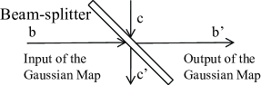
Figure 1: Gaussian Map constructed by a beam-splitter

Multi-mode extension.— Multi-mode Gaussian QPT has many important applications. For example, it applies to a complex linear optical circuit with BSs, squeezers, homodyne detections, linear losses, Gaussian noises and so on. Consider now a Gaussian process acting on a $k$-mode input state (on mode $b_{1},b_{2},\cdots b_{k}$), with outcome also a $k$-mode state. Even though other methods calgary can also be extended to the multi-mode case, the number of input states required there increases exponentially with the number of modes $k$, because the number of ket-bra operators $|\{n_{i}\}\rangle\langle\{m_{i}\}|$ in Fock space increases exponentially with $k$. As shown below, the number of input states in our method increases polynomially.

To apply isomorphism liusky , we consider $k$ pairs of maximally entangled states, each on modes $a_{1},b_{1}$; $a_{2},b_{2}$,$\cdots$ $a_{k},b_{k}$. Explicitly, $|\Phi^{+}\rangle=|\phi^{+}\rangle_{1}|\phi^{+}\rangle_{2}\cdots|\phi^{+}\rangle_{k}.$ Here $|\phi^{+}\rangle_{i}=\lim_{q\rightarrow 1}\exp\left({qa_{i}^{\dagger}b_{i}^{\dagger}}\right)|00\rangle$ indicates a maximally-entangled state on modes $a_{i},\;b_{i}$. Subspaces $a$ and $b$ each are now $k$-mode. Any state $|\psi\rangle$ in subspace $b$, can still be written in the form of Eq. (Efficient tomography of quantum processes), with the new definitions for $|\psi\rangle$ and $|\Phi^{+}\rangle$. Using Eq. (10), it is obvious that the output state of these $k$-pairs-TMSS fully characterize the process. A $k$-mode QPT can also be tested with $k$-mode CSs, if the process in Gaussian. The main Eqs. (22, 24) still hold after redefining the notations there. First, $\Gamma_{a},\;\Gamma_{b}$, $u$, $\alpha_{i}$, $d_{i}$, $Z_{a},Z_{b}$ are now $k$-mode vectors. For example, $|\alpha_{i}\rangle=|\alpha_{i1},\alpha_{i2},\cdots\alpha_{ik}\rangle$, $Z_{b}=(Z_{b1},Z_{b2},\cdots Z_{bk})$, $d_{i}=(d_{i1},d_{i2},\cdots d_{ik})$, and so on. Following Eq. (15), $\mathcal{X}_{xy}$ is now a $k\!\times\!k$ matrix, for $\mathcal{X}=X$ or $Y$ with $x=a,b$ $y=a,b$. We still apply Eqs. (22, 24) to calculate {$\Gamma_{b}$, $X_{ab},\;Y_{ab}$} and {$\Gamma_{a}$, $X_{aa}$, $Y_{aa}$}, respectively, but keep in mind that the matrices $K$, $J$ and symbols $d$, $c$ are now redefined. There are $(2k+1)k$ unknowns in ($\Gamma_{B},\;X_{ab},\;Y_{ab}$). We need $2k+1$ different CSs of $k$-mode to fix these unknowns. Matrix $K$ is now $(2k+1)\times(2k+1)$, since each $\alpha_{i}$ here is a $k$-mode row vector. Here $d$ is a $(2k+1)\times k$ matrix as $d^{T}=\left(d_{1}^{T},\;d_{2}^{T},\cdots d_{2k+1}^{T}\right)$, with $d_{i}=(d_{i1},d_{i2},\cdots d_{ik})$. Similarly, $J$ is now $N\times N$ and $N=(k+1)(2k+1)$, since $\alpha_{i}^{2}$ and $|\alpha_{i}|^{2}$ here are row vectors of $\alpha^{2}_{i}=(E_{i1},\;E_{i2},\cdots E_{ik})$ and $|\alpha_{i}|^{2}=(\tilde{E}_{i1},\;\tilde{E}_{i2},\cdots\tilde{E}_{ik})$, and each element of $E_{im}$ (or $\tilde{E}_{im}$) is a vector with ($k-m+1$) modes (or $k$ modes), as $E_{im}=(\alpha_{im}^{2},\alpha_{im}\alpha_{i,m+1},\alpha_{im}\alpha_{i,m+2},\cdots\alpha_{im}\alpha_{k},\alpha_{k}^{2})$ and $\tilde{E}_{im}=(\alpha_{im}\alpha^{*}_{i1},\alpha_{im}\alpha^{*}_{i2},\cdots\alpha_{im}\alpha^{*}_{i,k-1},\alpha_{im}\alpha^{*}_{ik})$. Obviously, $c$ is a column vector with $N$ elements. Therefore we conclude with this:
Corollary 1: Any $k$-mode map $\varepsilon$ in Fock space is characterized by the output state of $k$-pair-TMSS under one-sided map $I\otimes\varepsilon$. Any $k$-mode Gaussian QPT can be performed with $(k+1)(2k+1)$ different CSs of $k$-mode; or with $2k+1$ different CSs of $k$-mode if the process is trace-preserving.

In summary, we have presented explicit formulas quantum process characterization with only one weakly entangled state, as well as the tomography of a quantum optical Gaussian process with a few different coherent states. These results have been extended to multi-mode quantum optical process and the number of test states required increases only polynomially with the number of modes.

Acknowledgments XBW is supported by the NSFC under Grant No. 60725416, the National Fundamental Research Programs of China Grant No. 2007CB807900 and 2007CB807901, and China Hi-Tech Program Grant No. 2006AA01Z420. FN acknowledges partial support from the NSA, LPS, ARO, DARPA, NSF Grant No. 0726909, JSPS-RFBR Contract No. 09-02-92114, Grant-in-Aid for Scientific Research (S), MEXT Kakenhi on Quantum Cybernetics, and FIRST (Funding Program for Innovative R&D on S&T).

References

• (1) J.F. Poyatos, J.I. Cirac, and P. Zoller, Phys. Rev. Lett. 78, 390 (1997); G.M. D’Ariano and P. Lo Presti, Phys Rev. Lett. 86, 4195 (2001); M. Mohseni, A.T. Rezakhani, and D.A. Lidar, Phys. Rev. A 77, 032322 (2008).
• (2) K. Lobino et al, Science 322, 563 (2008); S. Rahimi-Keshari et al, arXiv:1009.3307v1.
• (3) A. Jamiolkowski, Rep. Math. Phys, 3, 275 (1972).
• (4) J. Eisert and M.B. Plenio, Phys. Rev. Lett. 89, 097901 (2002); G. Giedke and J.I. Cirac, Phys. Rev. A 66, 032316 (2002).