Brownian motors: Joint effect of non-Gaussian noise and time asymmetric forcing

Abstract

Previous works have shown that time asymmetric forcing on one hand, as well as non-Gaussian noises on the other, can separately enhance the efficiency and current of a Brownian motor. Here, we study the result of subjecting a Brownian motor to both effects simultaneously. Our results have been compared with those obtained for the Gaussian white noise regime in the adiabatic limit. We find that, although the inclusion of the time asymmetry parameter increases the efficiency value up to a certain extent, for the present case this increase is much less appreciable than in the white noise case. We also present a comparative study of the transport coherence in the context of colored noise. Though the efficiency in some cases becomes higher for the non-Gaussian case, the Péclet number is always higher in the Gaussian colored noise case than in the white noise as well as non-Gaussian colored noise cases.

I Introduction

In recent years noise induced transport by Brownian motors or “ratchets” review1 have attracted the attention of an increasing number of researchers. Such interest was motivated by their biological interest as well as for its potential technological applications. The pioneering works which included a built-in ratchet-like bias together with correlated fluctuations, were followed by works including and studying different aspects such as tilting and pulsating potentials, velocity inversions, etc. Thorough reviews in this area reiman indicate the biological and/or technological motivation for the study of ratchets as well as the state of the art. A large part of the contemporary literature points towards different means to improve the efficiency or the current in a ratchet system.

There are current studies on the role of non-Gaussian noises on some noise-induced phenomena qRE1 ; qRE1p ; qRE2 ; qruido1 ; qruido2 ; wio3 showing the possibility of strong effects on the system’s response. Such a noise source is based on the nonextensive statistics tsallis with a probability distribution that depends on $q$, a parameter indicating the departure from Gaussian behavior: for $q=1$ we have a Gaussian distribution, and different non-Gaussian distributions for $q>1$ or $q<1$. In qruido4 it was shown that the effect of such a non-Gaussian colored noise can strongly enhance the transport properties of Brownian motors.

Another line of work, also pointing towards efficiency enhancement, can be found in rk1 ; rk2 ; rk3 ; ai . The system considered in these works include both time and space asymmetries ajdari , thereby finding a range of parameters where a remarkable efficiency enhancement is obtained.

In the present work we explore the possibility of mixing up both previous enhancement methods. That is, to consider the system used in rk1 , but subject to a non-Gaussian colored noise source as used in qruido4 . As we indicate latter, it is in principle possible to try an analytical-like approach using an effective Markovian approximation qRE1 ; wio3 . However, here we have chosen to make an extensive numerical analysis of the problem. Moreover, as was shown in wio3 ; qruido4 , the enhancement is found to occur only for $q>1.0$, and for this reason we restrict our analysis only to such a finite range of the parameter $q$.

We also study the transport coherence in this model by analyzing the Péclet number $Pe$. This is a dimensionless number relevant in the study of transport phenomena, defined as the ratio of the rate of advection of a physical quantity by the flow to the rate of diffusion of the same quantity driven by an appropriate gradient landau . In our present case $Pe$ is defined as the ratio of current to the effective diffusion coefficient in the medium and is expressed as $Pe=\frac{l{v}}{D_{eff}},$ where $l$ is a characteristic length (in this case the length period=2$\pi$), $v$ the velocity, and $D_{eff}$ the (effective) diffusion coefficient. The transport of a Brownian particle is always accompanied by the spreading of fluctuations, namely, a diffusive spread, in the physical space at a fixed time, and the effectiveness of transport is affected by such a diffusive spread. The Brownian particle takes a time $t=l/v$ to traverse a distance $l$ with a velocity $v$ and the diffusive spread of the particle during the same time is given by $<(\Delta x)^{2}>=2D_{eff}t$. Hence, the criterion to have a reliable transport is that $<(\Delta x)^{2}>=2D_{eff}t<l^{2}$. This implies that $Pe=lv/D_{eff}>2$ for coherent transport pe . The value of $Pe$ depends on the characteristic length scale $l$ of the system.

Our results indicate that, even though we observe an enhancement in efficiency, in general it is smaller than for the white noise case. However, there are regions of parameters (like noise intensity, noise correlation time, departure from Gaussian behavior) that shows a remarkable optimization of the transport properties, that could have a strong interest for technological applications. Our results on $Pe$ shows that the inclusion of colored noise causes an enhancement in $Pe$ as compared to that in the white noise case, though, the value of $Pe$ is not high enough to make the net transport coherent over a wide range of parameter space. Also, Péclet number is always higher in the Gaussian colored noise case than in the non-Gaussian case at variance to the behavior of efficiency.

In the next section we describe the model, the noise source, and the simulation procedure. In section III we present our results and discuss them in detail. The last section includes some general conclusions and indications for future work.

II Model

We consider the motion of an overdamped Brownian particle subjected to a temporally asymmetric adiabatic forcing in the presence of a random noise source. The Langevin equation of motion of such a particle is

$$\frac{dx}{dt}=f(x)+F(t)-L+\zeta(t).$$ (1)

The periodic “ratchet” potential that we have adopted is $V(x)=-V_{0}\sin(x)-\mu/4\sin(2x)$, with the force field given by $f(x)=-dV(x)/dx$. Here, $\mu$ is a measure of the asymmetry in the periodic potential and we have scaled $V_{0}$ to be unity. The parameter $L$ in Eq. (1) is the external load force and $\zeta(t)$, that in the original formulation rk1 ; rk2 ; rk3 was assumed white, is a non-Gaussian colored noise governed by the equation

$$\frac{d\zeta(t)}{dt}=-\frac{1}{\sigma}\frac{dV_{q}(\zeta)}{d\zeta}+{\frac{1}{\sigma}\xi(t)},$$ (2)

where $\xi(t)$ is a zero mean and delta correlated ($<\xi(t)\xi(t^{\prime})>=2D\delta(t-t^{\prime})$) Gaussian white noise. The potential $V_{q}(\zeta)$ is

$$V_{q}(\zeta)=\frac{1}{\beta(q-1)}\ln\left(1+\beta(q-1)\frac{\zeta^{2}}{2}\right),$$ (3)

with $\beta=\sigma/D$. For $q=1$ we recover the Gaussian Ornstein-Uhlenbeck noise, a colored noise with time correlation $\sigma$. When $q=1$ and $\sigma=0$ we recover the Gaussian white noise case. Figure 1 in Refs. wio3 ; qruido4 depict the typical form of the probability distribution function for this process.

The periodic zero-mean forcing $F(t)$ in the above equation Langevin equation Eq. (1) is taken to be asymmetric in time and is given by

$$F(t) = \frac{1+\epsilon}{1-\epsilon}\,F_{0},\,\,\,\,\,\,\,\,\,\,\,\,n\tau\leq\,t\,<n\tau+\frac{1}{2}\tau(1-\epsilon),$$

$$= -F_{0},\,\,\,\,\,\,\,\,\,\,\,\,\,\,\,\,\,\,\,\,\,\,n\tau+\frac{1}{2}\tau(1-\epsilon)<\,t\,\leq(n+1)\tau.$$

Figure 1: Sketch of the time asymmetric forcing.

The parameter $\epsilon$ here characterizes the temporal asymmetry of the periodic forcing, $\tau$ is the time period of the driving force $F(t)$ and $n=0,1,..$ is an integer. We assume that $F(t)$ changes slow enough, i.e., its frequency is smaller than any other frequency related to the relaxation rate in the problem such that the system is in a steady state at each instant of time. Thus we consider the adiabatic limit of forcing and the profile of this forcing $F(t)$ is shown in Fig. 1.

Following the Stratonovich interpretation, the corresponding Fokker-Planck equation associated to Eqs. (1,2) is

$$\frac{\partial P_{q}(x,\zeta,\sigma,t)}{\partial t} = -\frac{\partial}{\partial x}\Bigl{(}[f(x)+F(t)-L+\zeta]P_{q}(x,\zeta,\sigma,t)\Bigr{)}$$ (5)

$$+ \frac{\partial}{\partial\zeta}\left(\frac{1}{\sigma}\left(\frac{d}{d\zeta}V_{q}(\zeta)\right)P_{q}(x,\zeta,\sigma,t)\right)+\frac{D}{\sigma^{2}}\frac{\partial^{2}}{\partial\zeta^{2}}P_{q}(x,\zeta,\sigma,t).$$

Since we are interested in the adiabatic limit it is possible to obtain an expression for the probability current density $j$ in the presence of a constant external force $F_{0}$ in the limit $q=1$ and $\sigma=0$. The expression is given by

$$j = \frac{1-\exp{[\frac{-2\pi F_{0}}{k_{B}T}]}}{{\int_{0}^{2\pi}dyI_{-}(y)}},$$ (6)

where $I_{-}(y)$ is given by

$$I_{-}(y)=\exp\,\left[\frac{-V(y)+F_{0}y}{k_{B}T}\right]\int_{y}^{y+2\pi}dx\exp\,\left[\frac{V(x)-F_{0}x}{k_{B}T}\right].$$ (7)

and $k_{B}T$ corresponds to the thermal noise which corresponds to $D$ in the present case. It may be noted that for $\mu=0$, $j(F_{0})\neq-j(-F_{0})$ for $\phi\neq 0\,,\,\pi$. This asymmetry ensures rectification of current for the rocked ratchet even in the presence of spatially symmetric potential.

The net current in the system arises due to the effect of the non-Gaussian noise as well as the zero mean time asymmetric forcing. The expression for the time averaged current due to the time asymmetric forcing alone can be separated into two parts

$$\langle j\rangle_{f}=j^{+}+j^{-},$$ (8)

where

$$j^{+} = \frac{1}{2}(1-\epsilon)\,j(\frac{1+\epsilon}{1-\epsilon}F_{0}),$$

$$j^{-} = \frac{1}{2}(1+\epsilon)\,j(-F_{0}).$$ (9)

Here, $j^{+}$ is the fraction of current that flows during the interval of time $(1-\epsilon)\frac{\tau}{2}$ when the external driving force is $\frac{1+\epsilon}{1-\epsilon}F_{0}$, and $j^{-}$ is the fraction of current that flows during the time period when the external driving force is $-F_{0}$. The difference between the total current, $J$, and the net current $\langle j\rangle_{f}$ from the time asymmetric forcing term, i.e., $j_{c}=J-\langle j\rangle_{f}$ comes from the colored non-Gaussian noise which in turn depends on $q$ and $\sigma$.

The contribution to the input energy also comes from both the colored noise and the time asymmetric forcing i.e., $E_{in}=E_{in-c}+E_{in-f}$. The input energy per unit time due to the time asymmetric forcing, $E_{in-f}$, can be expressed by kamegawa

$$E_{in-f}=\frac{1}{2}F_{0}\left[\left(\frac{1+\epsilon}{1-\epsilon}\right)j^{+}-j^{-}\right].$$ (10)

The contribution to the input energy from the non-Gaussian colored noise is given by qruido4

$$E_{in-c}=\lim_{t\rightarrow 0}\frac{1}{t}\int_{0}^{t}\zeta(t)\frac{dx}{dt}dt=\langle-V^{\prime}(x)\zeta\rangle+\langle\zeta^{2}\rangle,$$ (11)

where $\langle..\rangle$ indicates ensemble averaging. Numerical simulations show that the time average of $V^{\prime}(x(t))\zeta(t)$ (i.e., $\langle V^{\prime}(x(t))\zeta(t)\rangle$ ) is always several orders of magnitude smaller than $\langle\zeta(t)^{2}\rangle$ and hence such a term could be neglected. The quantity $\langle\zeta(t)^{2}\rangle$ can be approximated by $2D/{\sigma(5-3q)}$ qruido4 . Thus the expression for the contribution to the input energy from the non-Gaussian colored noise term is approximately given by

$$E_{in-c}\cong\frac{2D}{\sigma(5-3q)}.$$ (12)

It is worth to remark that this expression is valid only for finite values of $\sigma$ and hence is not applicable in the presence of an uncorrelated non-Gaussian noise source ($\sigma=0$ and $q\neq 0$).

The most common way of defining efficiency is by attaching a load force $L$ in a direction opposite to the direction of current in the ratchet eff-load . The overall potential experienced by the Brownian particle is then given by $V(x)=-V_{0}\sin(x)-(\mu/4)\,\sin(2x)+xL$. In order to reduce the number of parameters, in what follows we adopt the asymmetry parameter, $\mu=0$ or, in other words, the potential that the particle experience is a simple sinusoidal potential.

Within the operating range of the load, $0<L<L_{s}$, the particles move in a direction opposite to the direction of the applied load force thereby storing energy. $L_{s}$ indicates a threshold value (called stopping force) such that for $L=L_{s}$ the current is zero. The average work done over a period (i.e. power) is given by

$$E_{out}=\frac{1}{2}L\,J,$$ (13)

where $J$ is the total current rk1 ; rk2 .

The thermodynamic efficiency for energy transduction is given by

$$\eta=\frac{E_{out}}{E_{in}}\,.$$ (14)

As has been explained in rk1 , at low temperature, when the thermal energy is smaller than the modulation amplitude of the potential, $k_{B}T<V_{0}$, a significant current value can only arise when $F_{0}$, the external bias, is larger than a critical value which, in the present case, is $1$ riskin . When $F_{0}<1$, barriers exists in both directions and hence there is no current. A significant current can flow in the forward direction only when $\frac{1+\epsilon}{1-\epsilon}F_{0}>1$. Thus when $\frac{1-\epsilon}{1+\epsilon}<F_{0}<1$, a unidirectional current exists in the ratchet due to the temporally asymmetric periodic forcing. In the present work the value of the zero mean external bias $F_{0}$ lies in the range $0.11<F_{0}<1$.

III Numerical Details

We have numerically simulated Eqs. (1,2) using the Heun algorithm in the adiabatic limit for the external zero mean time asymmetric forcing (that is, the system follows the external forcing). The ratchet system is evolved for $10^{2}$ cycles of forcing, $t=10^{2}{\tau}$, where ${\tau}=10^{4}$ is the time period of forcing and the adopted time step is $10^{-2}$. This time period of external forcing is chosen to be large enough to ensure that we are in the limit of adiabatic forcing. We have done ensemble averages over $10^{3}$ trajectories and have calculated the current, diffusion, the efficiency and Péclet number, through numerical simulations. We have computed $v$, the net velocity, and $D_{eff}$, the effective diffusion coefficient describing fluctuations around the average position of the particles due to both the colored non-Gaussian noise as well as time asymmetric forcing and the Péclet number using the expressions

$$v=\Big{\langle}\,\frac{x(t)-x(t_{0})}{t-t_{o}}\,\Big{\rangle}=2\pi J,$$ (15)

and

$$D_{eff}=\lim_{t\to\infty}\frac{1}{2t}\left[\langle{x^{2}(t)}\rangle-{\langle x(t)\rangle}^{2}\right]$$ (16)

where $\langle\dots\rangle$, as in Eq. (11), denotes ensemble averaging. The Péclet number is given by

$$Pe=\frac{l{v}}{D_{eff}},$$ (17)

here $l$ is a characteristic length (=2$\pi$), $v$ the velocity, and $D_{eff}$ the (effective) diffusion coefficient. All the physical quantities are taken in dimensionless units.

IV Results and Discussions

We start by plotting in Fig. 2(a), and for different $q$ values, the efficiency as a function of load in presence of a temporally asymmetric forcing with $F_{0}=0.1$ and $\epsilon=0.8$. The adopted noise strength value was $D=0.1$ with a correlation time $\sigma=0.1$. We see a non-monotonous dependence of efficiency with load. For a fixed $q$ value, the efficiency increases with $L$, reaches a maximum value and then decreases. We observe that as we depart from Gaussian behavior, i.e., when $q$ departs from $1$ ($q>1$), the efficiency is found to increase up to a certain value of $q$ ($q=1.2$), and then it decreases when further increasing $q$. To be more specific, we find $\eta_{q=1.1}>\eta_{q=1.2}>\eta_{q=1.0}$. Also, the presence of non-Gaussian terms ($q>1$) reduces the range of operation of the ratchet. In the inset of the figure we show the behavior of efficiency with $q$ for the load value $L=0.05$. The load was chosen such that there was a finite efficiency value for all $q$. From the inset (b) we see that there is a small increase in efficiency up to $q=1.2$ followed by a strong decrease. Thus there is a non-monotonous behavior of efficiency with $q$ as we depart from the Gaussian case.

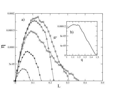
Figure 2: (a) Efficiency as a function of load for $F_{0}=0.1$, $\epsilon=0.8$, $D=0.1$ and $\sigma=0.1$ for different $q$ values: $q=1.0$ ($\circ$), $q=1.1$ ($\square$), $q=1.2$ ($\diamond$), $q=1.4$ ($+$), $q=1.5$ ($\ast$). The inset (b) shows the plot of efficiency with $q$ along the load value $L=0.05$.

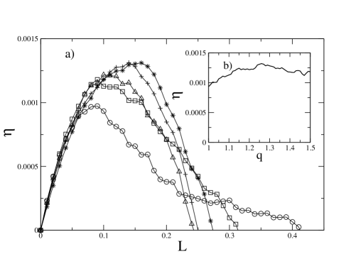
Figure 3: (a) Efficiency as a function of load for $F_{0}=0.1$, $\epsilon=0.8$, $D=0.1$ and $\sigma=1.0$ for different $q$ values: $q=1.0$ ($\circ$), $q=1.1$ ($\square$), $q=1.2$ ($\vartriangle$), $q=1.4$ ($+$), $q=1.5$ ($\ast$). The inset (b) shows the plot of efficiency with $q$ along the load value $L=0.1$.

In Fig. 3 (a) we plot the efficiency as a function of load for the same noise strength value, $D=0.1$, but with a larger correlation time $\sigma=1.0$, and all other parameters remaining the same. We observe that there is an increase in efficiency by an order of magnitude with increasing correlation time $\sigma$ when plotted as a function of load, $L$, i.e., $\eta_{max}=1.4\times 10^{-3}$. The inset shows the behavior of efficiency with $q$ when the load is $L=0.1$. We observe that there is an increase in efficiency when we depart from $q=1.0$, however, after $q\sim 1.25$, it slightly decreases, but much less markedly than in the inset of Fig. 2 (with $D=0.1$ and $\sigma=0.1$). Also, contrary to the behavior seen in Fig. 2, with lower correlation time and noise strength $D$, the efficiency in this case increases with increasing $q$. It should be noted that the maximum range of load is obtained for the Gaussian case. The higher $\sigma$ value helps in keeping the efficiency around a finite value. For an intermediate value of $\sigma$ ($\sigma=0.5$), we have seen that the efficiency value increases up to $q=1.2$, and at $q=1.3$ the efficiency drops to a value below the one we have at $q=1.0$, when plotted as a function of load (results not shown here). Beyond $q=1.3$ the efficiency again shoots up to a value above the Gaussian case.

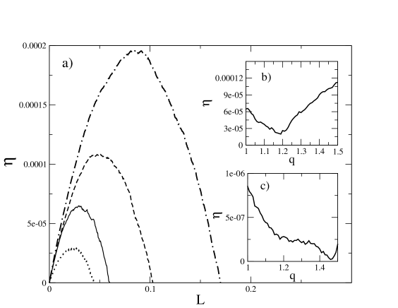
Figure 4: (a) Efficiency as a function of load for $F_{0}=0.1$, $\epsilon=0.8$, $D=1.0$ and $\sigma=1.0$ for different $q$ values: $q=1.0$ (solid line), $q=1.2$ (dotted line), $q=1.4$ (dashed line), $q=1.5$ (dash-dotted line). The inset (b) shows the behavior of efficiency with $q$ along the load value $L=0.03$ when $D=1.0$ and $\sigma=1.0$. The inset (c) shows the plot of efficiency with $q$ along the load value $L=0.003$ when $D=1.0$ and $\sigma=0.1$.

Figure 4 (a) shows efficiency plotted as a function of load for a larger noise strength value, $D=1.0$ and larger correlation time, $\sigma=1$ with all other parameters being the same. We see that as $q$ is increased, the efficiency value first decreases as $q$ goes from $q=1.0$ to $q=1.2$ and then the efficiency starts to increase. The important point to be noted here is that the efficiency value at $q=1.4$ is larger than that at $q=1.0$. This indicates that a correlation time $\sigma>0$ favors energy transduction in presence of a non-Gaussian noise ($q>1.0$). The interplay of $\sigma$ and $q$ gives rise to these interesting effects even when the noise strength $D$ is very high. The inset (b) in this figure shows the behavior of efficiency versus $q$ along the load value $L=0.03$. We can see that the efficiency decreases with increasing $q$ though there is a slight increase after $q=1.2$. However, this efficiency increase is much smaller than for the Gaussian colored noise case, $q=1$. Again, when $D=0.5$ and $\sigma=1.0$ the maximum efficiency is obtained when $q=1.0$. The inset (c) in this figure shows the plot of $\eta$ vs $q$ for $D=1.0$ and $\sigma=0.1$ for the load value $L=0.003$. We can see that the efficiency decreases with increasing $q$, reaches a minimum and then there is a small increase for $q=1.5$. The values are so small that the net efficiency value is almost negligible and hence we present here as an inset only the $\eta$ vs $q$ plot for which the appropriate load value has been chosen from the $\eta$ vs $L$ plot.

However we find that the maximum value for efficiency and the range of load is obtained for the Gaussian case, i.e. when $q=1$. As $q$ increases departing from the Gaussian case, the efficiency decreases up to $q=1.4$ and then increases for $q=1.5$, though this increase is much smaller than for $q=1.0$. Thus we can conclude that an increase in noise strength makes the system completely random and there is no directed transport possible in this range of parameters.

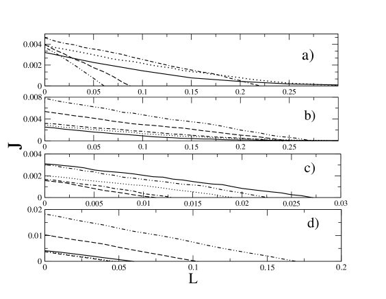
Figure 5: Current as a function of load for four particular cases, (a) $D=0.1$, $\sigma=0.1$, (b) $D=0.1$, $\sigma=1.0$, (c) $D=1.0$, $\sigma=0.1$ and (d) $D=1.0$, $\sigma=1.0$ with $F_{0}=0.1$ and $\epsilon=0.8$. The different lines correspond to: $q=1.0$ (solid), $q=1.1$ (dotted), $q=1.2$ (dash-dotted), $q=1.4$ (dashed), $q=1.5$ (dash-double dotted)).

In Fig. 5 we plot curves of current as a function of the load for the four cases of efficiency discussed above with different $q$ values. The figure caption gives the details of the values chosen for $D$ and $\sigma$. As expected, the current in the ratchet system decreases with an increase of the load force, and beyond a certain load value (the stopping force) the current starts to flow in the same direction as the load. The value of current, obtained in the presence of colored non-Gaussian noise, is much higher than that obtained in the presence of white noise. This is one of the main results to be stressed in our present work. From the curves we also see that except for the case of high noise strength and low correlation time, i.e., $D=1.0,\,\mbox{and}\sigma=0.1$, the value of current increases with an increase in $q$. The interplay of high noise strength and non-Gaussian behavior causes the current to be less than in the Gaussian case value. For the case $D=1.0$ and $\sigma=1.0$ the value obtained for the current was very high. In fact, the value of current decreases with $q$ up to $q=1.3$ and increases afterwards. However, we will not analyze this parameter range as a noise source with a large $\sigma$ value reduces the extent of randomness in the system.

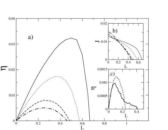
Figure 6: (a) Efficiency as a function of load for $D=0.1$, $\sigma=1.0$ and with $F_{0}=0.1$ and $\epsilon=0.9$. The inset (b) shows the behavior of current for the same set of parameters. The different lines correspond to: $q=1.0$ (solid), $q=1.2$ (dotted), $q=1.4$ (dashed), $q=1.5$ (dash-dotted)). The inset (c) shows the behavior of $\eta$ with load for $\epsilon=0.8$ and for $q=1.0$ (solid lines) and $q=1.2$ (dashed lines).

In Fig. 6 (a) we plot the variation of efficiency with load for the optimum value of system parameters, namely $\sigma=1.0$, $\epsilon=0.9$, $F_{0}=0.1$ and $D=0.1$. We see an enhancement in the efficiency for this specific range of parameters. As noted before, the efficiency keeps increasing when increasing $\sigma$. However, as indicated above, large values of $\sigma$ implies a more deterministic behavior of the system reentr forcing us to work with low $\sigma$ values. The inset (b) shows the behavior of current for the same set of parameters. The obtained value of current is high and it increases when we increase the departure from Gaussian behavior. But the stopping value of the load is high when noise source is colored and Gaussian.

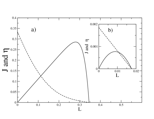
Figure 7: (a) Efficiency (solid line) and current (dotted line) as a function of load for the white noise case with $D=0.1$. The current is multiplied by a factor of 100 to scale with $\eta$. The inset (b) shows $\eta$ and current as a function of load for the case when $D=1.0$. The other parameter values chosen in the plot are $F_{0}=0.1$ and $\epsilon=0.8$.

To grasp the relevance of the time asymmetry parameter $\epsilon$, we checked the value of efficiency both with and without $\epsilon$. From the obtained results we could conclude that finite $\epsilon$ values contribute to the enhancement of efficiency even for correlated and non-Gaussian noise. However, this increase is still very small when compared with the increase in efficiency observed in the white noise case. We find that in order to have appreciable efficiency values, a large $\epsilon$ ($\epsilon\geq 0.6$) is needed. This means that the asymmetry in the temporal forcing has to be high which is in contrast with the white noise case.

We also see that efficiency is higher when $\epsilon=0.9$ than when $\epsilon=0.8$ by almost an order of magnitude for the same $q$ value. Thus for comparison, in the inset (c) of Fig. 6 we plot $\eta$ vs $L$ when $\epsilon=0.8$ with other parameters being the same. We represent here only two cases of efficiency value corresponding to $q=1.0$ and $q=1.2$. A similar behavior is seen for all other parameter ranges. We can clearly see that there is an enhancement in efficiency with higher $\epsilon$ values with a larger value being for the case when $q=1.0$. Thus we can conclude from Fig. 6 that the presence of correlation in noise reduces the efficiency value by a large amount even when the presence of barriers in one direction disappears due to the temporally asymmetric forcing parameter $\epsilon$.

In order to compare with the known results for the white noise case rk1 ; rk2 ; rk3 , in Fig. 7 we present the efficiency and the current in presence of white noise, as a function of load, and for two noise strength values (a) $D=0.1$ and (b) $D=1.0$. We see that an increase in $D$ causes the value of efficiency and also the range of load to be drastically reduced. The order of magnitude of current is almost the same and lies between $0.0015\sim 0.002$ for the case when $D=1.0$ and is between $0.003\sim 0.0035$ for the case when $D=0.1$.

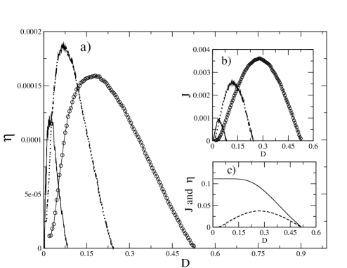
Figure 8: (a) Efficiency vs D for $\epsilon=0.8$, $L=0.1$ and $\sigma=0.1$ for different $q$ values: $q=1.0$ ($\circ$), $q=1.2$ (dotted), $q=1.4$ (solid). Inset (b) shows the behavior of current with $D$ for the same set of parameters. In the inset (c) we show the behavior of current (dashed) and efficiency (solid) for the white noise case as a function of noise strength $D$. Here the current is multiplied by a factor of 10 to scale with the efficiency value in the plot.

In Fig. 8 (a) we plot the efficiency as a function of noise strength $D$ with $\epsilon=0.8$, $L=0.1$, and $\sigma=0.1$, for different $q$ values. The inset (b) shows the dependence of the current with $D$ for the same set of parameters. We can see that both the current and efficiency show a peak as a function of $D$ for all range of parameters implying that noise facilitates energy transduction. To be more specific, both the efficiency and current are zero up to a certain value of $D$, beyond which there is a finite current and efficiency with a peak value for a particular $D$ in between and then with further increase in $D$ there is a reduction in current and efficiency. This is at variance with the behavior of efficiency in presence of white noise for both sinusoidal and sawtooth potential rk1 ; rk2 ; rk3 .

The existence of a peak in efficiency with $D$ can be understood by plotting the curves of input energy and current as a function of the noise intensity $D$ for the corresponding set of parameters. On increasing $D$, the current starts to rise to a larger value as compared to zero temperature value, and there is also an increase in efficiency. However, when $D$ increases beyond a certain value, there will be a contribution to the current in both directions, due to the overcoming of the potential barrier in either directions, implying a reduction of the net current. As a result, the efficiency will in turn has to decrease in the high temperature regime.

The shift in the efficiency maximum when departing from Gaussian regime is apparent from the plot. Such a maximum in $\eta$ has a non-monotonic behavior, with the largest value occurring for $q=1.2$, while the current maxima, as a function of $D$, has a monotonic nature. The maximum value of the current decreases when departing from Gaussian regime as is seen in inset (b) of this figure.

To have a comparison with the white noise case, in Fig. 8 we have included an inset (c) where we show the behavior of efficiency and current with a sinusoidal potential, subjected only to white noise. We see that for this case, though the current has a maximum as a function of $D$ the efficiency does not show a maximum. Only a fine tuning of the different parameters could yield a maximum in the current and efficiency with $D$. This is in contrast with that for the colored noise case where it is possible to obtain a peak in $\eta$ and $J$ with $D$ for both Gaussian and non-Gaussian noises, though the peak value of efficiency and current are very small.

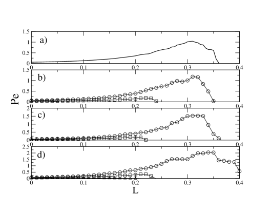
Figure 9: Plot of $Pe$ as a function of load for four different cases of interest: (a) white noise case, (b) $D=0.1$ and $\sigma=0.01$, (c) $D=0.1$ and $\sigma=0.1$, (d) $D=0.1$ and $\sigma=1.0$. Other parameters are $\epsilon=0.8$ and $q=1.0$ ($\circ$), $q=1.2$ ($\square$) and $q=1.4$ ($\vartriangle$)).

Finally we analyze the transport coherence by calculating the Péclet number ($Pe$) and make a comparison with the white noise case. Fig. 9 shows the behavior of $Pe$ as a function of the load for the cases of interest in this work. It is apparent that the inclusion of colored noise causes an enhancement in $Pe$ as compared to that in the white noise case, though the value of $Pe$ is not high enough to make the net transport coherent.

From the above plot we can also observe that though the value of $Pe$ is not high to make the transport coherent, the best value of $Pe$ is always obtained in the Gaussian colored noise case. In other words, though the efficiency in some cases becomes higher for the non-Gaussian case, the Péclet number is always high in the Gaussian case. The inclusion of non-Gaussianity makes the transport less and less coherent.

A final observation from the above plot is that the $Pe$ approaches a value of $2$ for a small range of load values for the case when $D=0.1$ and $\sigma=1.0$. Thus, as in the case of efficiency, an increase in $\sigma$ makes the transport to be coherent. We can conclude that in the Gaussian colored noise case it is possible to have a larger transport coherence than in the white noise case (i.e., with the inclusion of $\sigma$), due to the larger current. However, the efficiency value reduces with the inclusion of $\sigma$.

V Conclusions

We have studied the combined effect of a non-Gaussian colored noise source and a zero mean temporal asymmetric rocking force on crucial quantities of the ratchet system, namely the current, efficiency and Péclet number. We have seen that though time asymmetric forcing helps to increase the efficiency, such an increase is not as appreciable as in the white noise regimes. However, we have found that there exists a parameter regime for noise intensity, noise correlation time, and departure from Gaussian behavior, showing a notable optimization of the transport properties, that could have a strong interest for technological applications.

Finally, a direct analytic approach, exploiting an effective Markovian approximation qRE1 ; qRE1p is possible, but highly cumbersome from a numerical point of view. Another possibility that we are trying to implement is a perturbation approach for small $\sigma$ and for $q\sim 1$ (i,e, $|q-1|\ll 1$). We expect that such an approach will reveal some details about the behavior of the system in relation to the role of the different parameters on efficiency and current. In particular, we expect it could clarify how the two enhancement methods interacts leading to a poor enhancement when combined. Such studies will be the subject of a forthcoming work futur .

- (1) R. D. Astumian, Science 276, 917 (1997).
- (2) P. Reimann, Phys. Rep. 361, 57 (2002), P. Hänggi and F. Marchesoni, Rev. Mod. Phys. 81, 387 (2009); see also A. M. Jayannavar, cond-mat 0107079.
- (3) M.A. Fuentes, R. Toral and H.S. Wio, Physica A 295, 114-122 (2001); M.A. Fuentes, H.S. Wio and R. Toral, Physica A 303, 91–104 (2002).
- (4) M.A. Fuentes, C. Tessone, H.S. Wio and R. Toral, Fluctuations and Noise Letters 3, L365 (2003).
- (5) F.J. Castro, M.N. Kuperman, M.A. Fuentes and H.S. Wio, Phys. Rev. E 64, 051105 (2001).
- (6) H.S. Wio, J.A. Revelli and A.D. Sánchez, Physica D 168-169, 165-170 (2002).
- (7) H.S. Wio and R. Toral, in Anomalous Distributions, Nonlinear Dynamics and Nonextensivity, H. Swineey and C. Tsallis (Eds.), Physica D 193, 161 (2004).
- (8) H.S. Wio, On the Role of Non-Gaussian Noises, in Nonextensive Entropy-Interdisciplinary Applications, M.Gell-Mann and C. Tsallis, Eds. (Oxford U.P., Oxford, 2003).
- (9) C. Tsallis, Stat. Phys. 52, 479 (1988); E.M.F. Curado and C. Tsallis, J. Phys. A 24, L69 (1991); ibid, 24, 3187 (1991); ibid, 25, 1019 (1992).
- (10) S. Bouzat and H.S. Wio, Eur. Phys. J. B. 41, 97-105 (2004); S. Bouzat and H.S. Wio, Physica A 351, 69-78 (2005).
- (11) R. Krishnan, M.C. Mahato and A.M. Jayannavar, Phys. Rev. E 70, 021102 (2004).
- (12) R. Krishnan, S. Roy and A.M. Jayannavar, J. Stat. Mech. P04012 (2005).
- (13) R. Krishnan, J. Chacko. M. Sahoo and A.M. Jayannavar, J. Stat. Mech. P06017 (2006).
- (14) B.-Q. Ai, X. J. Wang, G. T. Liu, D. H. Wen, H. Z. Xie, W. Chen and L. G. Liu, Phys. Rev. E 68, 061105 (2003).
- (15) A. Ajdari, D. Mukamel, L. Peliti and J. Prost, J. Phys. I France 4, 1551 (1994), M.C. Mahato and A.M. Jayannavar, Phys. Lett. A 209, 21 (1995), D.R. Chialvo, M.M. Millonas, Phys. Lett. A 209, 26 (1995), M.C. Mahato, T.P. Pareek and A.M. Jayannavar, Int. J. Mod. Phys. B 10, 3857 (1996).
- (16) L. D. Landau and E. M. Lifshitz, Fluid Dynamics, Pergamon Press, Oxford, 1959.
- (17) S. Roy, D. Dan and A. M. Jayannavar, J. Stat. Mech. P09012 (2006); R. Krishnan, D. Dan and A. M. Jayannavar, Mod. Phys. Lett. B 19 Nos 19 & 20, 971 (2005); R. Krishnan, D. Dan and A. M. Jayannavar, Physica A 354, 171 (2005); B. Linder and L Schimansky-Geier, Phys. Rev. Lett. 89, 230602 (2002), R. Krishnan, D. Dan and A. M. Jayannavar, Ind. J. Phys. 78, 747 (2004), J. A. Freund and L. Schimansky-Geier, Phys. Rev. E60, 1304 (1999); K. Visscher, M. J. Schnitzer and S. M. Block, Nature 400, 184 (1999), T. Harms and R. Lipowsky, Phys. Rev. Lett. 79, 2895 (1997), M. J. Schnitzer and S. M. Block, Nature (London) 388, 386 (1997).
- (18) H. Kamegawa, T. Hondou and F. Takagi, Phys. Rev. Lett. 80, 5251 (1998); F. Takagi and T. Hondou, Phys. Rev. E60, 4954 (1999); D. Dan and A. M. Jayannavar, Phys. Rev. E66, 41106 (2002).
- (19) K. Sekimoto, J. Phys. Soc. Jpn. 66, 6335 (1997); J. M. R. Parrondo and B. J. De Cisneros, Appl. Phys. A75, 179 (2002).
- (20) H. Risken, The Fokker-Planck Equation (Springer Verlag, Berlin 1984).
- (21) F. Castro, A. Sánchez and H.S.Wio, Phys. Rev. Lett. 75, 1691 (1995).
- (22) R. Krishnan and H.S. Wio, in preparation.