Optional Pólya tree and Bayesian inference

Abstract

We introduce an extension of the Pólya tree approach for constructing distributions on the space of probability measures. By using optional stopping and optional choice of splitting variables, the construction gives rise to random measures that are absolutely continuous with piecewise smooth densities on partitions that can adapt to fit the data. The resulting “optional Pólya tree” distribution has large support in total variation topology and yields posterior distributions that are also optional Pólya trees with computable parameter values.

Optional Polya tree and Bayesian inference

and

t1Supported in part by NSF Grants DMS-05-05732 and DMS-09-06044. t2Supported by a Gerhard Casper Stanford Graduate Fellowship.

62F15, 62G99, 62G07, Polya tree, Bayesian inference, nonparametric, recursive partition, density estimation

1 Introduction

Ferguson ferg73 formulated two criteria for desirable prior distributions on the space of probability measures: (i) The support of the prior should be large with respect to a suitable topology, and (ii) the corresponding posterior distribution should be analytically manageable. Extending the work by Freedman free63 and Fabius fabius64 , he introduced the Dirichlet process as a prior that satisfies these criteria. Specifically, assuming for simplicity that the parameter space $\Omega$ is a bounded interval of real numbers, and the base measure in the Dirichlet process prior is the Lebesgue measure, then the prior will have positive probability in all weak neighborhoods of any absolutely continuous probability measure, and given i.i.d. observations, the posterior distribution is also a Dirichlet process with its base measure obtainable from that of the prior by the addition of delta masses at the observed data points.

While these properties made it an attractive prior in many Bayesian nonparametric problems, the use of the Dirichlet process prior is limited by its inability to generate absolutely continuous distributions; that is, a random probability measure sampled from the Dirichlet process prior is almost surely a discrete measure black73 , blackmac73 , ferg73 . Thus in applications that require the existence of densities under the prior, such as the estimation of a density from a sample lo84 or the modeling of error distributions in location or regression problems dia86 , there is a need for alternative ways to specify the prior. Lo lo84 proposed an elegant prior in the space of densities by assuming the density is a mixture of kernel functions where the mixing distribution is modeled by a Dirichlet process. Under Lo’s model, the random distributions are guaranteed to have smooth densities and the predictive density is still analytically tractable. However the degree of smoothness is not adaptive.

Another approach to deal with the discreteness problem is to use Pólya tree priors ferg74 . This class of random probability measures includes the Dirichlet process as a special case and yet is itself a special case of the more general class of “tail free” processes previously studied by Freedman free63 . Pólya tree prior satisfies Ferguson’s two criteria. First, it is possible to construct Pólya tree priors with positive probability in neighborhoods around arbitrary positive densities lav92 . Second, the posterior distribution arising from a Pólya tree prior is available in close form ferg74 . Further properties and applications of Pólya tree priors are found in hutter09 , lav94 , ghosh03 , hans06 and maul92 .

In this paper we study the extension of the Pólya tree prior construction by allowing optional stopping and randomized partitioning schemes. To motivate optional stopping, consider the standard construction of the Pólya tree prior for probability measures in an interval $\Omega$. The interval is recursively bisected into subintervals. At each stage, the probability mass already assigned to an interval is randomly divided and assigned into its subintervals according to the independent draw of a Beta variable. However, in order for the prior to generate absolutely continuous measures, it is necessary for the parameters in the Beta distribution to increase rapidly as the depth of the bisection increases, that is, as we move into more and more refined levels of partitioning kraft64 .

In any case, even when the construction yields a random distribution with density, with probability $1$ the density will have discontinuity almost everywhere. The use of Beta variables with large magnitudes for its parameters, although useful in forcing the random distribution to be absolutely continuous, has the effect of severely constraining our ability to allocate conditional probability to represent faithfully the data distributions within small intervals. To resolve this conflict between smoothness and faithfulness to the data distribution, one can introduce an optional stopping variable for each subregion obtained in the partitioning process hutter09 . By putting uniform distributions within each stopped subregion, we can achieve the goal of generating absolutely continuous distributions without having to force the Beta parameters to increase rapidly. In fact, we will be able to use Jeffrey’s rule of Beta ($\frac{1}{2},\frac{1}{2}$) in the inference of conditional probabilities, regardless of the depth of the subregion in the partition tree. We believe this is a desirable consequence of optional stopping.

Our second extension is to allow randomized partitioning. Standard Pólya tree construction relies on a fixed scheme for partitioning. For example in hans06 a $k$-dimensional rectangle is recursively partitioned where in each stage of the recursion the subregions are further divided into $2^{k}$ quadrants by bisecting each of the $k$ coordinate variables. In contrast, when recursive partitioning is used in other statistical problems, it is customary to allow flexible choices of the variables to use to further divide a subregion. This allows the subregion to take very different shapes depending on the information in the data. The data-adaptive nature of the recursive partitioning is a reason for the success of tree-based learning methodologies such as CART brei84 . Thus it is desirable to allow Pólya tree priors to use partitions that are the result of randomized choices of divisions in each of the subregions at each stage of the recursion. Once the partitioning is randomized in the prior, the posterior distribution will give more weights on those partitions that provide better fits to the data. In this way the data is allowed to influence the choice of the partitioning. This will be especially useful in high-dimensional applications.

In Section 2 we introduce the construction of “Optional Pólya trees” that allow optional stopping and randomized partitioning. It is shown that this construction leads to priors that give absolutely continuous distributions almost surely. We also show how to specify the prior so that it has positive probability in all total variation neighborhoods in the space of absolutely continuous distributions on $\Omega$. In Section 3 we show that the use of optional Pólya tree priors will lead to posterior distributions that are also optional Pólya trees. We present a recursive algorithm for the computation of the parameters governing the posterior optional Pólya tree. These results ensure that Ferguson’s two criteria are satisfied by optional Pólya tree priors, but now on the space of absolutely continuous probability measures. In this section, we also show that the posterior Pólya tree is weakly consistent in the sense that asymptotically it concentrates all its probability in any weak neighborhood of a true distribution whose density is bounded. In Section 4, we develop and test the optional Pólya tree approach to density estimation in Euclidean space. Concluding remarks are given in Section 5.

We end this introduction with brief remarks on related works. The important idea of early stopping was first introduced by Hutter hutter09 . Ways to attenuate the dependency of Pólya trees on the partition include mixing the base measure used to define the tree lav92 , lav94 , hans06 , random perturbation of the dividing boundary in the partition of intervals paddock03 and the use of positively correlated variables for the conditional probabilities at each level of the tree definition (Nieto-Barajas and Müller BarajasandMuller2009 ). Compared to these works, our approach allows not only early stopping but also randomized choices of the splitting variables. This provides a much richer class of partitions than previous models and raises the new challenge of learning the partition based on the observed data. We show that under mild conditions such learning is achievable by finite computation. We also provide a relatively complete mathematical foundation which represents the first theory for Bayesian density estimation based on recursive partitioning. Although a Bayesian version of recursive partitioning has been proposed previously (Bayesian CART, denison98 ), it was formulated for a different problem (classification instead of density estimation). Furthermore, it studied mainly model specification and computational algorithm, and did not discuss the mathematical and asymptotic properties of the method.

2 Optional Pólya tree

We are interested in constructing random probability measures on a space $(\Omega,\mu)$. $\Omega$ is either finite or a bounded rectangle in $\mathbb{R}^{p}$. In this paper we assume for simplicity that $\mu$ is the counting measure in the finite case and the Lebesgue measure in the continuous case. Suppose that $\Omega$ can be partitioned in $M$ different ways; that is, for $j=1,2,\ldots,M$,

$$\Omega=\bigcup_{k=1}^{K^{j}}\Omega_{k}^{j}\qquad\mbox{where }\Omega_{k}^{j}\mbox{'s are disjoint}.$$

Each $\Omega_{k}^{j}$, called a level-1 elementary region, can in turn be divided into level-2 elementary regions. Assume there are $M_{k_{1}}^{j_{1}}$ ways to divide $\Omega_{k_{1}}^{j_{1}}$; then for $j_{2}=1,\ldots,M_{k_{1}}^{j_{1}}$, we have

$$\Omega_{k_{1}}^{j_{1}}=\bigcup_{k_{2}=1}^{K_{k_{1}}^{j_{1}j_{2}}}\Omega_{k_{1}k_{2}}^{j_{1}j_{2}}.$$

In general, for any level-$k$ elementary region $A$, we assume there are $M(A)$ ways to partition it; that is, for $j=1,2,\ldots,M(A)$,

$$A=\bigcup_{k=1}^{K^{j}(A)}A_{k}^{j}.$$

Let $\mathcal{A}^{k}$ be the set of all possible level-$k$ elementary regions, and $\mathcal{A}^{(k)}=\bigcup_{l=1}^{k}\mathcal{A}^{l}$. If $\Omega$ is finite, we assume that $\mathcal{A}^{k}$ separates points in $\Omega$ if $k$ is large enough. If $\Omega$ is a rectangle in $\mathbb{R}^{p}$, we assume that every open set $B\subset\Omega$ is approximated by unions of sets in $\mathcal{A}^{(n)}$, that is, $\exists B_{n}\uparrow B$ where $B_{n}$ is a finite union of disjoint regions in $\mathcal{A}^{(n)}$.

Example 1.

$$\Omega = \bigl{\{}x=(x_{1},\ldots,x_{p})\dvtx x_{i}\in\{1,2\}\bigr{\}},$$

$$\Omega_{k}^{j} = \{x\dvtx x_{j}=k\},\qquad k=1\mbox{ or }2,$$

$$\Omega_{k_{1}k_{2}}^{j_{1}j_{2}} = \{x\dvtx x_{j_{1}}=k_{1},x_{j_{2}}=k_{2}\},\qquad\mbox{ etc.}$$

In this example, the number of ways to partition a level-$k$ elementary region decreases as $k$ increases.

Example 2.

$$\Omega=\{(x_{1},x_{2},\ldots,x_{p})\dvtx x_{i}\in[0,1]\}\subset\mathbb{R}^{p}.$$

If $A$ is a level-$k$ elementary region (a rectangle), and $m_{j}(A)$ is the midpoint of the range of $x_{j}$ for $A$, we set $A_{1}^{j}=\{x\in A\dvtx x_{j}\leq m_{j}(A)\}$ and $A_{2}^{j}=A\setminus A_{1}^{j}$. There are exactly $M(A)=p$ ways to partition each $A$, regardless of its level.

Once a system to generate partitions has been specified as above, we can formally define recursive partitions as follows. A recursive partition of depth $k$ is a series of decisions $J^{(k)}=(J_{1},J_{2},\ldots,J_{k})$ where $J_{l}$ represents all the decisions made at level $l$ to decide, for each region produced at the previous level, whether or not to stop partitioning it further and if not, which way to use to partition it. Once we have decided not to partition a region, then it will remain intact at all subsequent levels. Thus each $J^{(k)}$ specifies a partition of $\Omega$ into a subset of regions in $\mathcal{A}^{(k)}$.

We use a recursive procedure to produce a random recursive partition of $\Omega$ and a random probability measure $Q$ that is uniformly distributed within each part of the partition. Suppose after $k$ steps of the recursion, we have obtained a random recursive partition $\mathbf{J}^{(k)}$ and we write

$$\Omega=T_{0}^{k}\cup T_{1}^{k},$$

where

$$T_{0}^{k} = \bigcup_{i=1}^{I}A_{i}\qquad\mbox{is a union of disjoint }A_{i}\in\mathcal{A}^{(k-1)},$$

$$T_{1}^{k} = \bigcup_{i=1}^{I^{\prime}}A^{\prime}_{i}\qquad\mbox{is a union of disjoint }A^{\prime}_{i}\in\mathcal{A}^{k}.$$

The set $T_{0}$ represents the part of $\Omega$ where the partitioning has already been stopped and $T_{1}$ represents the complement. In addition, we have also obtained a random probability measure $Q^{(k)}$ on $\Omega$ which is uniformly distributed within each region in $T_{0}^{k}$ and $T_{1}^{k}$.

In the $(k+1)$th step, we define $Q^{(k+1)}$ by further partitioning of the regions in $T_{1}^{k}$ as follows. For each elementary region $A$ in the above decomposition of $T_{1}^{k}$, generate an independent random variable,

$$S\sim\operatorname{Bernoulli}(\rho).$$

If $S=1$, stop further partitioning of $A$ and add it to the set of stopped regions. If $S=0$, draw $J\in\{1,2,\ldots,M(A)\}$ according to a nonrandom vector $\bolds\lambda(A)=(\lambda_{1},\ldots,\lambda_{M(A)})$, called the selection probability vector, that is, $P(J=j)=\lambda_{j}$ and $\sum_{l=1}^{M(A)}\lambda_{l}=1$. If $J=j$, apply the $j$th way of partitioning $A$,

$$A=\bigcup_{l=1}^{K}A_{l}^{j}\qquad\mbox{(here $K$ depends on $A$ and $j$)}$$

and set $Q^{(k+1)}(A_{l}^{j})=Q^{(k)}(A)\theta_{l}^{j}$ where $\bolds\theta^{j}=(\theta_{1}^{j},\ldots,\theta_{K}^{j})$ is generated from a Dirichlet distribution with parameter $(\alpha_{1}^{j},\ldots,\alpha_{K}^{j})$. The nonrandom vector $\bolds\alpha^{j}=\bolds\alpha^{j}(A)$ is referred to as the assignment weight vector.

After this step, we have obtained $T_{0}^{k+1}$ and $T_{1}^{k+1}$, the respective unions of the stopped and continuing regions. Clearly

$$\Omega = T_{0}^{k+1}\cup T_{1}^{k+1},$$

$$T_{0}^{k+1} \supset T_{0}^{k},\qquad T_{1}^{k+1}\subset T_{1}^{k}.$$

The new measure $Q^{(k+1)}$ is then defined as a refinement of $Q^{(k)}$. For $B\subset T_{0}^{(k+1)}$, we set

$$Q^{(k+1)}(B)=Q^{(k)}(B).$$

For $B\subset T_{1}^{(k+1)}$ where $T_{1}^{k+1}$ is partitioned as

$$T_{1}^{k+1}=\bigcup_{i=1}^{J}A_{i},\qquad A_{i}\in\mathcal{A}^{k+1},$$

we set

$$Q^{(k+1)}(B)=\sum_{i=1}^{J}Q^{(k+1)}(A_{i})\biggl{(}\frac{\mu(A_{i}\cap B)}{\mu(A_{i})}\biggr{)}.$$

Recall that for each $A_{i}$ in the partition of $T_{1}^{k+1}$, we have already generated its $Q^{(k+1)}$ probability.

Let $\mathcal{F}^{(k)}$ be the $\sigma$-field of events generated by all random variables used in the first $k$ steps; the stopping probability $\rho=\rho(A)$ is required to be measurable with respect to $\mathcal{F}^{(k)}$. The specification of $\rho(\cdot)$ is called the stopping rule. In this paper we are mostly interested in the case when $\rho(\cdot)$ is an “independent stopping rule;” that is, $\rho(A)$ is a pre-specified constant for each possible elementary region $A$. However in some applications it is useful to let $\rho(A)$ depend on $Q^{(k)}(A)$.

Let $\mathcal{A}^{(\infty)}=\bigcup_{k=1}^{\infty}\mathcal{A}^{k}$ be the set of all possible elementary regions.

Theorem 1.

Suppose there is a $\delta>0$ such that with probability $1$, $1-\delta>\rho(A)>\delta$ for any region $A$ generated during any step in the recursive partitioning process. Then with probability $1$, $Q^{(k)}$ converges in variational distance to a probability measure $Q$ that is absolutely continuous with respect to $\mu$.

Definition 1.

The random probability measure $Q$ defined in Theorem 1 is said to have an optional Pólya tree distribution with parameters $\bolds\lambda,\bolds\alpha$ and stopping rule $\rho$.

Proof of Theorem 1 We only need to prove this for the case when $\Omega$ is a bounded rectangle. We can think of $Q^{(k)}$’s as being generated in two steps.

1. Generate the nonstopped version $Q^{*(k)}$ by recursively choosing the ways of partitioning each level of regions but without stopping in any of the regions. Let $J^{*(k)}$ denote the decision made during this process in the first $k$ levels of the recursion. Each realization of $J^{*(k)}$ determines a partition of $\Omega$ consisting of regions $A\in\mathcal{A}^{k}$ (not $\mathcal{A}^{(k)}$ as in the case of optional stopping). Let $\mathcal{A}^{k}(J^{*(k)})=\{A\in\mathcal{A}^{k}\dvtx A$ is a region in the partition induced by $J^{*(k)}\}$. If $A\in\mathcal{A}^{k}(J^{*(k)})$, then it can be written as

   $$A=\Omega_{l_{1}l_{2}\cdots l_{k}}^{j_{1}j_{2}\cdots j_{k}}.$$

   We set

   $$Q^{*(k)}(A)=\theta_{l_{1}}^{j_{1}}\cdot\theta_{l_{1}l_{2}}^{j_{1}j_{2}}\cdots\theta_{l_{1}\cdots l_{k}}^{j_{1}\cdots j_{k}}\quad\mbox{and}\quad Q^{*(k)}(\cdot|A)=\mu(\cdot|A).$$

   This defines $Q^{*(k)}$ as a random measure.

2. Given the results in Step 1, generate the optional stopping variables $S=S(A)$ for each region $A\in\mathcal{A}^{k}(J^{*(k)})$, successively for each level $k=1,2,3,\ldots.$ Then for each $k$, modify $Q^{*(k)}$ to get $Q^{(k)}$ by replacing $Q^{*(k)}(\cdot|A)$ with $\mu(\cdot|A)$ for any stopped region $A$ up to level $k$.

For each $A\in\mathcal{A}^{k}(J^{*(k)})$, let $I^{k}(A)=$ indicator of the event that $A$ has not been stopped during the first $k$ levels of the recursion:

$$E\bigl{(}Q^{(k)}(T_{1}^{k})|J^{*(k)}\bigr{)} = E\biggl{(}\sum_{A\in\mathcal{A}^{k}(J^{*(k)})}Q^{*(k)}(A)I^{k}(A)|J^{*(k)}\biggr{)}$$

$$= \sum_{A\in\mathcal{A}^{k}(J^{*(k)})}E\bigl{(}Q^{*(k)}(A)|J^{*(k)}\bigr{)}E\bigl{(}I^{k}(A)|J^{*(k)}\bigr{)}$$

$$\leq (1-\delta)^{k}\sum_{A\in\mathcal{A}^{k}(J^{*(k)})}E\bigl{(}Q^{*(k)}(A)|J^{*(k)}\bigr{)}$$

$$= (1-\delta)^{k}.$$

Thus $E(Q^{(k)}(T_{1}^{k}))\to 0$ geometrically and hence $Q^{(k)}(T_{1}^{k})\to 0$ with probability $1$. Similarly, $\mu(T_{1}^{k})\to 0$ with probability $1$.

For any Borel set $B\subset\Omega$, we claim that $\lim Q^{(k)}(B)$ exists with probability $1$. To see this, write

$$Q^{(k)}(B) = Q^{(k)}(B\cap T_{0}^{k})+Q^{(k)}(B\cap T_{1}^{k})$$

$$= a_{k}+b_{k};$$

$a_{k}$ is increasing since

$$Q^{(k+1)}(B\cap T_{0}^{k+1}) \geq Q^{(k+1)}(B\cap T_{0}^{k})$$

$$= Q^{(k)}(B\cap T_{0}^{k}),$$

and $b_{k}\to 0$ since $Q^{(k)}(T_{1}^{k})\to 0$ with probability $1$.

Since the Borel $\sigma$-field $\mathcal{B}$ is generated by countably many rectangles, we have with probability $1$ that $\lim Q^{(k)}(B)$ exists for all $B\in\mathcal{B}$. Define $Q(B)$ as this limit. If $Q(B)>0$ then $Q^{(k)}(B)>0$ for some $k$. Since $Q^{(k)}\ll\mu$ by construction, we must also have $\mu(B)>0$. Thus $Q$ is absolutely continuous.

For any $B\in\mathcal{B}$, $Q^{(k)}(B\cap T_{0}^{k})=Q(B\cap T_{0}^{k})$, and hence

$$\bigl{|}Q^{(k)}(B)-Q(B)\bigr{|} = \bigl{|}Q^{(k)}(B\cap T_{1}^{k})-Q(B\cap T_{1}^{k})\bigr{|}$$

$$< 2Q^{(k)}(T_{1}^{k})\longrightarrow 0.$$

Thus the convergence of $Q^{(k)}$ to $Q$ is in variational distance.

The next result shows that it is possible to construct optional Pólya tree distribution with positive probability on all $L_{1}$ neighborhoods of densities.

Theorem 2.

Let $\Omega$ be a bounded rectangle in $\mathbb{R}^{p}$. Suppose that the condition of Theorem 1 holds and that the selection probabilities $\lambda_{i}(A)$, the assignment probabilities $\alpha_{i}^{j}(A)/(\sum_{l}\alpha_{l}^{j}(A))$ for all $i,j$ and $A\in\mathcal{A}^{(\infty)}$ are uniformly bounded away from $0$ and $1$. Let $q=dQ/d\mu$; then for any density $f$ and any $\tau>0$, we have

$$P\biggl{(}\int|q(x)-f(x)|\,d\mu<\tau\biggr{)}>0.$$

First assume that $f$ is uniformly continuous. Let

$$\delta(\varepsilon)={\sup_{|x-y|<\varepsilon}}|f(x)-f(y)|;$$

then $\delta(\varepsilon)\downarrow 0$ as $\varepsilon\downarrow 0$. For any $k$ large enough, we can find a partitioning $\Omega=\bigcup_{i=1}^{I}A_{i}$ where $A_{i}\in\mathcal{A}^{k}$ is arrived at by $k$ steps of recursive partitioning (deterministic and without stopping) and that each $A_{i}$ has diameter $<\varepsilon$.

Approximate $f$ by a step function $f^{*}(x)=\sum_{i}f_{i}^{*}I_{A_{i}}(x),f_{i}^{*}=\int_{A_{i}}f\,d\mu/\break\mu(A_{i})$. Let $D_{\varepsilon}(f)$ be the set of step functions $g(\cdot)=\sum g_{i}I_{A_{i}}(\cdot)$ satisfying

$${\sup_{i}}|g_{i}-f_{i}^{*}|<\delta(\varepsilon).$$

Suppose $g\in D_{\varepsilon}(f)$; then for any $B$ we have $B=\bigcup_{i=1}^{I}(B\cap A_{i})=\bigcup_{i=1}^{I}B_{i}$ and

$$\biggl{|}\int_{B}(g-f)\,d\mu\biggr{|} \leq \sum_{i}|g_{i}-f_{i}^{*}|\mu(B_{i})+\sum_{i}\biggl{|}f_{i}^{*}\mu(B_{i})-\int_{B_{i}}f\,d\mu\biggr{|}$$

$$\leq \sum_{i}\delta(\varepsilon)\mu(B_{i})+\sum_{i}r_{i},$$

where

$$r_{i} = \mu(B_{i})\biggl{|}\frac{\int_{A_{i}}f\,d\mu}{\mu(A_{i})}-\frac{\int_{B_{i}}f\,d\mu}{\mu(B_{i})}\biggr{|}$$

$$= \mu(B_{i})\biggl{|}\frac{\int_{A_{i}}(f(x)-f(x_{k}))\,d\mu}{\mu(A_{i})}-\frac{\int_{B_{i}}(f(x)-f(x_{k}))\,d\mu}{\mu(B_{i})}\biggr{|},$$

where $x_{i}\in B_{i}$. Since

$$|f(x)-f(x_{i})|<\delta(\varepsilon)\qquad\mbox{for }x\in A_{i},$$

we have

$$|r_{i}|<2\delta(\varepsilon)\mu(B_{i}).$$

Hence

$$\biggl{|}\int_{B}(g-f)\,d\mu\biggr{|}<3\delta(\varepsilon)\mu(B)\qquad\forall B,$$

and thus

$$\int|g-f|\,d\mu<3\delta(\varepsilon)\mu(\Omega)=3\delta^{\prime}(\varepsilon),$$

where $\delta^{\prime}(\varepsilon)=\delta(\varepsilon)\mu(\Omega)$. Since all probabilities in the construction of $q^{k}=\frac{dQ^{(k)}}{d\mu}$ are bounded away from $0$ and $1$, we have

$$P\bigl{(}q^{k}\in D_{\varepsilon}(f)\mbox{ for all large }k\bigr{)}>0.$$

Hence

$$P\biggl{(}\int|q^{k}-f|\,d\mu<3\delta^{\prime}(\varepsilon)\mbox{ for all large }k\biggr{)}>0.$$

On the other hand, by Theorem 1, we have

$$P\biggl{(}\int|q^{k}-q|\,d\mu\to 0\biggr{)}=1.$$

Thus

$$P\biggl{(}\int|q-f|\,d\mu<4\delta^{\prime}(\varepsilon)\biggr{)}>0.$$

Finally, the result also holds for a discontinuous $f$ since we can approximate it arbitrarily closely in $L_{1}$ distance by a uniformly continuous one.

It is not difficult to specify $\alpha_{i}^{j}(A)$ to satisfy the assumption of Theorem 2. A useful choice is

$$\alpha_{i}^{j}(A)=\tau^{k}\mu(A_{i}^{j})/\mu(\Omega)\qquad\mbox{for }A\in\mathcal{A}^{k},$$

where $\tau>0$ is a suitable constant.

The reason for including the factor $\tau^{k}$ when $A\in\mathcal{A}^{k}$ is to ensure that the strength of information we specified for the conditional probabilities within $A$ is not diminishing as the depth of partition $k$ increases. For example, in Example 2 each $A$ is partitioned into two parts of equal volumes; that is,

$$A=A_{1}^{j}\cup A_{2}^{j},\qquad\mu(A_{1}^{j})=\mu(A_{2}^{j})=\tfrac 12\mu(A).$$

Thus $A\in\mathcal{A}^{k}\Rightarrow\mu(A_{i}^{j})=2^{-(k+1)}\mu(\Omega)$, and

$$\alpha_{i}^{j}(A)=2^{k}\frac{\mu(A_{i}^{j})}{\mu(\Omega)}=\frac{1}{2}\qquad\mbox{for all }k.$$

In this case, by choosing $\tau=2$ we have obtained a nice “self-similarity” property for the optional Pólya tree, in the sense that the conditional probability measure $Q(\cdot|A)$ will have an optional Pólya tree distribution with the same specification for $\alpha_{i}^{j}$’s as in the original optional Pólya tree distribution for $Q$.

Furthermore, in this example if we use $\tau=2$ to specify a prior distribution for Bayesian inference of $Q$, then for any $A\in\mathcal{A}^{k}$, the inference for the conditional probability $\theta_{1}^{j}(A)$ will follow a classical binomial Bayesian inference with the Jeffrey’s prior Beta ($\frac{1}{2},\frac{1}{2}$).

3 Bayesian inference with an optional Pólya tree prior

Suppose we have observed $\mathbf{x}=\{x_{1},x_{2},\ldots,x_{n}\}$ where $x_{i}$’s are independent draws from a probability measure $Q$, where $Q$ is assumed to have an optional Pólya tree as a prior distribution. In this section we show that the posterior distribution of $Q$ given $\mathbf{x}$ also follows an optional Pólya tree distribution.

We denote the prior distribution for $q=\frac{dQ}{d\mu}$ by $\pi(\cdot)$. For any $A\subset\Omega$, we define $\mathbf{x}(A)=\{x_{i}\in\mathbf{x}\dvtx x_{i}\in A\}$ and $n(A)=\#(\mathbf{x}(A))=$ cardinality of the set $\mathbf{x}(A)$. Let

$$q(x)=\frac{dQ}{d\mu}(x)\qquad\mbox{for }x\in\Omega$$

and

$$q(x|A)=\frac{q(x)}{Q(A)}\qquad\mbox{for }x\in A;$$

then the likelihood for $\mathbf{x}$ and the marginal density for $\mathbf{x}$ can be written, respectively, as

$$P(\mathbf{x}|Q) = \prod_{i=1}^{n}q(x_{i})=q(\mathbf{x}),$$

$$P(\mathbf{x}) = \int q(\mathbf{x})\,d\pi(q).$$

The variable $q$ (or $Q$) represents the whole set of random variables, that is, the stopping variable $S(A)$, the selection variable $J(A)$ and the condition probability allocation $\theta_{i}^{j}(A)$, etc., for all regions $A$ generated during the generation of the random probability measure $Q$.

In what follows, we assume that the stopping rule needed for $Q$ is an independent stopping rule. By considering how $\Omega$ is partitioned and how probabilities are assigned to the parts of this partition, we have

$$q(\mathbf{x})=Su(\mathbf{x})+(1-S)\Biggl{(}\prod_{i=1}^{K^{J}}(\theta_{i}^{J})^{n_{i}^{J}}\Biggr{)}q(\mathbf{x}|\mathbf{N}^{J}=\mathbf{n}^{J}).$$ (1)

In this expression:

$u(\mathbf{x})=\prod_{i=1}^{n}u(x_{i})$ where $u(x)=\frac{1}{\mu(\Omega)}$ is the uniform density on $\Omega$.

$S=S(\Omega)$ is the stopping variable for $\Omega$.

$J$ is the choice of partitioning to use on $\Omega$.

$\mathbf{N}^{J}=(n(\Omega_{1}^{J}),\ldots,n(\Omega_{K^{J}}^{J}))$ is the counts of observations in $\mathbf{x}$ falling into each part of the partition $J$.

To understand $q(\mathbf{x}|\mathbf{N}^{J}=\mathbf{n}^{j})$, suppose $J=j$ specifies a partition $\Omega=\Omega_{1}^{j}\cup\Omega_{2}^{j}\cup\cdots\cup\Omega_{K^{j}}^{j}$; then the sample $\mathbf{x}$ is partitioned accordingly into subsamples,

$$\mathbf{x}=\mathbf{x}(\Omega_{1}^{j})\cup\cdots\cup\mathbf{x}(\Omega_{K^{j}}^{j}).$$

Under $Q$, if the subsample sizes $n_{1}^{j},\ldots,n_{K^{j}}^{j}$ are given, then the positions of points in $\mathbf{x}(\Omega_{i}^{j})$ within $\Omega_{i}^{j}$ are generated independently of those in the other subregions. Thus

$$q(\mathbf{x}|\mathbf{N}^{J}=n^{j})=\prod_{i=1}^{K^{j}}q(\mathbf{x}(\Omega_{i}^{j})|\Omega_{i}^{j}),$$

where

$$q(\mathbf{x}(\Omega_{i}^{j})|\Omega_{i}^{j})=\prod_{x\in\mathbf{x}(\Omega_{i}^{j})}q(x|\Omega_{i}^{j}).$$

Note that once $J=j$ is given, $q(\cdot|\Omega_{i}^{j})$ is generated independently as an optional Pólya tree according to the parameters $\bolds\rho,\bolds\lambda,\bolds\alpha$ that are relevant within $\Omega_{i}^{j}$. We denote by $\Phi(\Omega_{i}^{j})$ the expectation of $q(\mathbf{x}(\Omega_{i}^{j})|\Omega_{i}^{j})$ under this induced optional Pólya tree within $\Omega_{i}^{j}$.

In fact, for any $A\subset\bigcup_{k=1}^{\infty}\mathcal{A}^{k}$, we have an induced optional Pólya tree distribution $\pi_{A}(q)$ for the conditional density $q(\cdot|A)$, and we define

$$\Phi(A)=\int q(\mathbf{x}(A)|A)\,d\pi_{A}(q),$$

if $\mathbf{x}(A)\neq\varnothing$ and $\Phi(A)=1$ if $\mathbf{x}(A)=\varnothing$. Similarly, we define

$$\Phi_{0}(A)=u(\mathbf{x}(A)|A)=\prod_{x\in\mathbf{x}(A)}u(x|A)$$

and $\Phi_{0}(A)=1$ if $\mathbf{x}(A)=\varnothing$. Note that $P(\mathbf{x})=\Phi(\Omega)$ and $u(\mathbf{x})=\Phi_{0}(\Omega)$.

Next, we successively integrate out [w.r.t. $\pi(\cdot)$] the random variables in the right-hand side of (1) according to the order $q(\mathbf{x}|\mathbf{n}^{J}),\bolds\theta^{J},J$ and $S$ (last). This gives us

$$\Phi(\Omega)=\rho\Phi_{0}(\Omega)+(1-\rho)\sum_{j=1}^{M}\lambda_{j}\frac{D(\mathbf{n}^{j}+\bolds\alpha^{j})}{D(\bolds\alpha^{j})}\prod_{i=1}^{K^{j}}\Phi(\Omega_{i}^{j}),$$ (2)

where $D(\mathbf{t})=\Gamma(t_{1})\cdots\Gamma(t_{k})/\Gamma(t_{1}+\cdots+t_{k})$.

Similarly, for any $A\in\bigcup_{k=1}^{\infty}\mathcal{A}^{k}$ with $\mathbf{x}(A)\neq\varnothing$, we have

$$\Phi(A)=\rho\Phi_{0}(A)+(1-\rho)\sum_{j=1}^{M}\lambda_{j}\frac{D(\mathbf{n}^{j}+\bolds\alpha^{j})}{D(\bolds\alpha^{j})}\prod_{i=1}^{K^{j}}\Phi(A_{i}^{j}),$$ (3)

where $\mathbf{n}^{j}$ is the vector of counts in the partition $A=\bigcup_{i=1}^{K^{j}}A_{i}^{j}$, and $M,K^{j},\rho,\bolds\lambda^{j}$, $\bolds\alpha^{j}$, etc., all depend on $A$. We note that in the special case when the choice of splitting variables are nonrandom, a similar recursion was given in hutter09 .

We can now read off the posterior distribution of $S=S(\Omega)$ from equation (2) by noting that the first term $\rho\Phi_{0}(\Omega)$ and the remainder in the right-hand side of (2) are, respectively, the probabilities of the events

{stopped at $$\Omega \mathbf{x} u(\cdot)$$, generate from }

and

{not stopped at $$\Omega \mathbf{x} M$$, generate by one of the partitions}.

Thus $S\sim$ Bernoulli with probability $\rho\Phi_{0}(\Omega)/\Phi(\Omega)$. Similarly, the $j$th term in the sum (over $j$) appearing in the right-hand side of (2) is the probability of the event

{not stopped at $$\Omega \mathbf{x} j \Omega$$, generate by using the th way to partition }.

Hence, conditioning on not stopping at $\Omega$, $J$ takes value $j$ with probability proportional to

$$\lambda_{j}\frac{D(\mathbf{n}^{j}+\bolds\alpha^{j})}{D(\bolds\alpha^{j})}\prod_{i=1}^{K^{j}}\Phi(\Omega_{i}^{j}).$$

Finally, given $J=j$, the probabilities assigned to the parts of this partition are $\bolds\theta^{j}$ whose posterior distribution is Dirichlet ($\mathbf{n}^{j}+\bolds\alpha^{j}$).

By similar reasoning, we can also read off the posterior distribution of $S=S(A),J=J(A),\bolds\theta^{j}=\bolds\theta^{j}(A)$ from (3) for any $A\subset\mathcal{A}^{k}$. Thus we have proven the following.

Theorem 3.

Suppose $\mathbf{x}=(x_{1},\ldots,x_{n})$ are independent observations from $Q$ where $Q$ has a prior distribution $\pi(\cdot)$ that is an optional Pólya tree with independent stopping rule, and satisfying the condition of Theorem 2, the conditional distribution of $Q$ given $\mathbf{X}=\mathbf{x}$ is also an optional Pólya tree where, for each $A\subset A^{\infty}$, the parameters are given as follows:

1. Stopping probability:

   $$\rho(A|\mathbf{x})=\rho(A)\Phi_{0}(A)/\Phi(A).$$

2. Selection probabilities:

   $$P(J=j|\mathbf{x})\propto\lambda_{j}\frac{D(\mathbf{n}^{j}+\bolds\alpha^{j})}{D(\bolds\alpha^{j})}\prod_{i=1}^{K^{j}}\Phi(A_{i}^{j}),\qquad j=1,\ldots,M.$$

3. Allocation of probability to subregions: the probabilities $\theta_{i}^{j}$ for subregion $A_{i}^{j},i=1,\ldots,K^{j}$ are drawn from Dirichlet ($\mathbf{n}^{j}+\bolds\alpha^{j}$).

In the above, it is understood that $M,K^{j},\lambda_{j},\mathbf{n}^{j},\bolds\alpha^{j}$ all depend on $A$.

We use the notation $\pi(\cdot|x_{1},x_{2},\ldots,x_{n})$ to denote this posterior distribution for $Q$.

To use Theorem 3, we need to compute $\Phi(A)$ for $A\in\mathcal{A}^{\infty}$. This is done by using the recursion (3), which says that $\Phi(\cdot)$ is determined for a region $A$ if it is first determined for all subregions $A_{i}^{j}$. By going into subregions of increasing levels of depth, we will eventually arrive at some regions having certain simple relations with the sample $\mathbf{x}$. We can often derive close form solutions for $\Phi(\cdot)$ for such “terminal regions” and hence determine all the parameters in the specifications of the posterior optional Pólya tree by a finite computation. We give two examples.

Example 3 (($2^{p}$ contingency table)).

Let $\Omega=\{1,2\}\times\{1,2\}\times\cdots\times\{1,2\}$ be a table with $2^{p}$ cells. Let $\mathbf{x}=(x_{1},x_{2},\ldots,x_{n})$ be $n$ independent observations where each $x_{i}$ falls into one of the $2^{p}$ cells according to the cell probabilities $\{q(y)\dvtx y\in\Omega\}$. Assume that $q$ has an optional Pólya tree distribution according to the partitioning scheme in Example 1 where $\lambda_{j}=\frac{1}{M}$ if there are $M$ variables still available for further splitting of a region $A$, and $\alpha_{i}^{j}=\frac{1}{2},i=1,2$. Finally, assume that $\rho(A)\equiv\rho$ where $\rho\in(0,1)$ is a constant.

In this example, there are three types of terminal regions.

1. $A$ contains no observation. In this case, $\Phi(A)=1$.

2. $A$ is a single cell (in the $2^{p}$ table) containing any number of observations. In this case, $\Phi(A)=1$.

3. $A$ contains exactly one observation, and $A$ is a region where $M$ of the $p$ variables are still available for splitting. In this case,

   $$\Phi(A)=r_{M}=\int q(x)\,d\pi_{M}(Q),$$

   where $\pi_{M}(\cdot)$ is the optional Pólya tree on a $2^{M}$ table. By recursion (3) we have

   $$r_{M} = \rho 2^{-M}+(1-\rho)\Biggl{(}\frac{1}{M}\sum_{j=1}^{M}\frac{B(3/2,1/2)}{B(1/2,1/2)}\Biggr{)}\cdot r_{M-1}$$

   $$= \rho 2^{-M}+(1-\rho)\frac{1}{2}r_{M-1}$$

   $$= \rho 2^{-M}\frac{(1-(1-\rho)^{M})}{1-(1-\rho)}+\biggl{(}\frac{1-\rho}{2}\biggr{)}^{M}$$

   $$= 2^{-M}.$$

Example 4.

$\Omega$ is a bounded rectangle in $\mathbb{R}^{p}$ with a partitioning scheme as in Example 2. Assume that for each region, one of the $p$ variables is chosen to split it $(\lambda_{j}\equiv\frac{1}{p})$, and that $\alpha_{i}^{j}=\frac{1}{2},i=1,2$. Assume $\rho(A)$ is a constant, $\rho\in(0,1)$. In this case, a terminal region $A$ contains either no observations [then $\Phi(A)=1$] or a single observation $x\in A$. In the latter case,

$$\Phi(A)=r_{A}(x)=\int_{A}q(x|A)\,d\pi_{A}(Q)$$

and

$$r_{A}(x) = \frac{\rho}{\mu(A)}+(1-\rho)\frac{1}{p}\sum_{j=1}^{p}\frac{B(3/2,1/2)}{B(1/2,1/2)}\cdot r_{A_{i(x)}^{j}}(x)$$

$$= \frac{\rho}{\mu(A)}+(1-\rho)\frac{1}{2}r_{A_{i(x)}^{j}}(x),$$

where $i(x)=1$ or $2$ according to whether $x\in A_{1}^{j}$ or $A_{2}^{j}$. Since $\mu(A_{1}^{j})=\mu(A_{2}^{j})=\frac{1}{2}\mu(A)$ for the Lebesgue measure, we have

$$r_{A}(x) = \frac{\rho}{\mu(A)}+(1-\rho)\frac{1}{2}\biggl{[}\frac{\rho}{\mu(A)\cdot 1/2}+(1-\rho)\frac{1}{2}[\cdots]\biggr{]}$$

$$= \frac{\rho}{\mu(A)}[1+(1-\rho)+(1-\rho)^{2}+\cdots]$$

$$= \frac{1}{\mu(A)}.$$

Example 5.

$\Omega$ is a bounded rectangle in $\mathbb{R}^{p}$. At each level, we split the regions according to just one coordinate variable, according to a predetermined order; for example, coordinate variable $x_{i}$ is used to split all regions at the $k$th step whenever $k\equiv i$ (mod $p$). In this case, $\Phi(A)$ for terminal regions are determined exactly as in Example 4. By allowing only one way to split a region, we sacrifice some flexibility in the resulting partition in exchange for a great reduction of computational complexity.

Our final result in this section shows that optional Pólya tree priors lead to posterior distributions that are consistent in the weak topology. For any probability measure $Q_{0}$ on $\Omega$, a weak neighborhood $U$ of $Q_{0}$ is a set of probability measures of the form

$$U=\biggl{\{}Q\dvtx\biggl{|}\int g_{i}(\cdot)\,dQ-\int g_{i}(\cdot)\,dQ_{0}\biggr{|}<\varepsilon_{i},i=1,2,\ldots,K\biggr{\}},$$

where $g_{i}(\cdot)$ is a bounded continuous function on $\Omega$.

Theorem 4.

Let $x_{1},x_{2},\ldots$ be independent, identically distributed variables from a probability measure $Q$, $\pi(\cdot)$ and $\pi(\cdot|x_{1},\ldots,x_{n})$ be the prior and posterior distributions for $Q$ as defined in Theorem 3. Then, for any $Q_{0}$ with a bounded density, it holds with $Q_{0}^{(\infty)}$ probability equal to $1$ that

$$\pi(U|x_{1},\ldots,x_{n})\longrightarrow 1$$

for all weak neighborhoods $U$ of $Q_{0}$.

It is a consequence of Schwarz’s theorem schw65 that the posterior is weakly consistent if the prior has positive probability in Kullback–Leibler neighborhoods of the true density ghosh03 , Theorem 4.4.2. Thus, by the same argument as in Theorem 2, we only need to show that it is possible to approximate a bounded density in Kullback–Leibler distance by step functions on a suitably refined partition.

Let $f$ be a density satisfying $\sup_{x\in\Omega}f(x)\leq M<\infty$. First assume that $f$ is continuous with modulus of continuity $\delta(\varepsilon)$. Let $\bigcup_{i=1}^{I}A_{i}$ be a recursive partition of $\Omega$ satisfying $A_{i}\in\mathcal{A}^{k}$ and diameter $(A_{i})\leq\varepsilon$. Let

$$g_{i}=\sup_{x\in A_{i}}f(x),\qquad g(x)=\sum_{i=1}^{I}g_{i}I_{A_{i}}(x)$$

and $G=\int g(x)\,d\mu$. We claim that as $\varepsilon\to 0$, the density $g/G$ approximates $f$ arbitrarily well in Kullback–Leibler distance. To see this, note that

$$0 \leq G-1=\int(g-f)\,d\mu=\sum_{i}\int_{A_{i}}\bigl{(}g(x)-f(x)\bigr{)}\,d\mu$$

$$\leq \sum_{i}\int_{A_{i}}\delta(\varepsilon)\,d\mu=\delta(\varepsilon)\mu(\Omega).$$

Hence

$$0 \leq \int f\log\bigl{(}f/(g/G)\bigr{)}\,d\mu$$

$$= \int f\log(f/g)\,d\mu+\int f\log G\,d\mu$$

$$\leq \log(G)\leq\log\bigl{(}1+\delta(\varepsilon)\mu(\Omega)\bigr{)}.$$

Finally, if $f$ is not continuous, we can find a set $B\subset\Omega$ with $\mu(B^{c})<\varepsilon^{\prime}$ such that $f$ is uniformly continuous on $B$. Then

$$\int(g-f)\,d\mu = \int_{B}(g-f)\,d\mu+\int_{B^{c}}(g-f)\,d\mu$$

$$\leq \delta(\varepsilon)\mu(\Omega)+M\varepsilon^{\prime}$$

and the result still holds.

4 Density estimation using an optional Pólya tree prior

In this section we develop and test the methods for density estimation using an optional Pólya tree prior. Two different strategies are considered. The first is through computing the posterior mean density. The other is a two-stage approach—first learn a fixed tree topology that is representative of the underlying structure of the distribution, and then compute a piecewise constant estimate conditional on this tree topology. Our numerical examples start with the one-dimensional setting to demonstrate some of the basic properties of optional Pólya trees. We then move onto the two-dimensional setting to provide a flavor of what happens when the dimensionality of the distribution increases.

4.1 Computing the mean

For the purpose of demonstration, we first consider the situation described in Example 2 with $p=1$ where the state space is the unit interval and the splitting point of each elementary region (or tree node) is the middle point of its range. In this simple scenario, each node has only one way to divide, so the only decision to make is whether to stop or not. Each point $x$ in the state space $\Omega$ belongs to one and only one elementary region in $A^{k}$ for each $k$. In this case, the posterior mean density function can be computed very efficiently using an inductive procedure. (See the Appendix for details.)

In a multi-dimensional setting with multiple ways to split at each node, the sets in each $A^{k}$ could overlap, and so the computation of the posterior mean is more difficult. One way to get around this problem is to place some restriction on how the elementary regions can split. For example, an alternate splitting rule requires that each dimension is split in turn (Example 5). This limits the number of choices to split for each elementary region to one and effectively reduces the dimensionality of the problem to one. However, in restricting the ways to divide, one wastes a lot of computation on cutting dimensions that need not be cut which affects the variability of the estimate significantly. We demonstrate this phenomenon in our later examples.

Another way to compute (or at least approximate) the posterior mean density is first explored by Hutter hutter09 . For any point $x\in\Omega$, Hutter proposed computing $\Phi(\Omega|x,D)$ and using $\Phi(\Omega|x,D)/\Phi(\Omega|D)$ as an estimate of the posterior mean density at $x$. [Here $D$ represents the observed data; $\Phi(\Omega|D)$ denotes the $\Phi$ computed for the root node given the observed data points and $\Phi(\Omega|x,D)$ is computed treating $x$ as an extra data point observed.] This method is general but computationally intensive, especially when there are multiple ways to divide each node. Also, because this method is for estimating the density at a specific point, to investigate the entire function one must evaluate $\Phi(\Omega|x,D)$ on a grid of $x$ values which makes it even more unattractive computationally. For this reason, in our later two-dimensional examples we only use the restriction method discussed above to compute the posterior mean.

4.2 The hierarchical MAP method

Another approach for density estimation using an optional Pólya tree prior is to proceed in two steps—first learn a “good” partition or tree topology over the state space, and then estimate the density conditional on this tree topology. The first step reduces the prior process from an infinite mixture of infinite trees to a fixed finite tree. Given such a fixed tree topology (i.e., whether to stop or not at each step, and if not, which way to divide), we can easily compute the (conditional) mean density function. The posterior probability mass over each node is simply a product of Beta means, and the distribution within those stopped regions is uniform by construction. So the key lies in learning a reliable tree structure. In fact, learning the tree topology is useful beyond facilitating density estimation. A representative partition over the state space by itself sheds light on the underlying structure of the distribution. Such information is particularly valuable in high-dimensional problems where direct visualization of the data is difficult.

Because a tree topology depends only on the decisions to stop and the ways to split, its posterior probability is determined by the posterior $\rho$’s and $\lambda$’s. The likelihood of each fixed tree topology is the product of a sequence of terms in the form, $\rho$, $1-\rho$, $\lambda_{k}$, depending on the stopping and splitting decisions at each node. One seemingly obvious candidate tree topology for representing the data structure is the maximum a posteriori (MAP) topology, that is, the topology with the highest posterior probability. However, in this setting the MAP topology often does not produce the most descriptive partition for the distribution. It biases toward shorter tree branches in that deeper tree structures simply have more terms less than 1 to multiply into their posterior probability. While the data typically provide strong evidence for the stopping decisions (and so the posterior $\rho$’s for all but the very deep nodes are either very close to 1 or very close to 0), this is not the case for the $\lambda$’s. It occurs often that for an elementary region the data points are distributed relatively symmetrically in two or more directions, and thus the posterior $\lambda$’s for those directions will be much less than 1. As a consequence, deep tree topologies, even if they reflect the actual underlying data structure, often have lower posterior probabilities than shallow trees do. (This failure of the MAP estimate relates more generally to the multi-modality of the posterior distribution as well as the self-similarity of the prior process and deserves more studies in its own right.)

We propose the construction of the representative tree topology through a simple top-down sequential procedure. Starting from the root node, if the posterior $\rho>0.5$ then we stop the tree; otherwise we divide the tree in the direction $k$ that has the highest $\lambda_{k}$. (When there is more than one direction with the same highest $\lambda_{k}$, the choice among them is arbitrary.) Then we repeat this procedure for each $A_{k}^{j}$ until all branches of the tree have been stopped. This can be viewed as a hierarchical MAP decision procedure—with each MAP decision being made based on those made in the previous steps. In the context of building trees, this approach is natural in that it exploits the hierarchy inherent in the problem.

4.3 Numerical examples

Next we apply the optional Pólya tree prior to several examples of density estimation in one and two dimensions. We consider the situation described in Example 2 with $p=1$ and $2$ where the state space is the unit interval $[0,1]$ and the unit square $[0,1]\times[0,1]$, respectively. The cutting point of each coordinate is the middle point of its range for the corresponding elementary region. For all the optional Pólya tree priors used in the following examples, the prior stopping probability $\rho=0.5$ and the prior pseudo-count $\alpha=0.5$ for all elementary regions. The standard Pólya tree priors examined (as a comparison) have quadratically increasing pseudo-counts $\alpha=\operatorname{depth}^{2}$ (see ferg74 and kraft64 ). For numerical purpose, we stop dividing the nodes if their support is under a certain threshold which we refer to as the precision threshold. We used $10^{-6}$ as the precision threshold in the one-dimensional examples and $10^{-4}$ in the two-dimensional examples. Note that in the 1D examples, each node has only one way to divide, and so we can use the inductive procedure described in the Appendix to compute the posterior mean density function. For the 2D examples, we implemented and tested the full optional tree as well as a restricted version based on “alternate cutting” (see Example 5).

Example 6 ((Mixture of two close spiky uniforms)).

We simulate data from the following mixture of uniforms:

$$0.5U(0.23,0.232)+0.5U(0.233,0.235)$$

and we apply three methods to estimate the density function. The first is to compute the posterior mean density using an optional Pólya tree prior. The second is to apply the hierarchical MAP method using an optional Pólya tree prior. The third is to compute the posterior mean using a standard Pólya tree prior. The results are presented in Figure 1. Several points can be made from this figure. (1) A sample size of 500 is

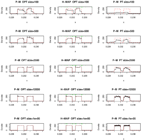
Figure 1: Density estimation for $0.5U(0.23,0.232)+0.5U(0.233,0.235)$. The five rows represent five different sample sizes $n=100$, 500, 2500, 12,500 and 100,000. The first column corresponds to the posterior mean approach using an optional Pólya tree prior. The second column corresponds to the hierarchical MAP method using an optional Pólya tree prior. The green ticks along the top margins of this column indicate the partition learned from this method. The third column corresponds to the posterior mean approach using a standard Pólya tree prior with $\alpha=\operatorname{depth}^{2}$. The red dashed lines in all plots represent the true density function.

sufficient for the optional tree methods to capture the boundaries as well as the modes of the uniform distributions whereas the Pólya tree prior with quadratic pseudo-counts requires thousands of data points to achieve this. (2) With increasing sample size, the estimates from the optional Pólya tree methods become smoother, while the estimate from the standard Pólya tree with quadratic pseudo-counts is still “locally spiky” even for a sample size of $10^{5}$. (This problem can be remedied by increasing the prior pseudo-counts faster than the quadratic rate at the price of further loss of flexibility.) (3) The hierarchical MAP method performs just as well as the posterior mean approach even though it requires much less computation and memory. (4) The partition learned in the hierarchical MAP approach reflects the structure of the distribution.

Example 7 ((Mixture of two Betas)).

Next we apply the same three methods to simulated samples from a mixture of two Beta distributions,

$$0.7\operatorname{Beta}(40,60)+0.3\operatorname{Beta}(2000,1000).$$

The results are given in Figure 2. Both the

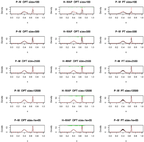
Figure 2: Density estimation for $0.7\operatorname{Beta}(40,60)+0.3\operatorname{Beta}(2000,1000)$. The five rows represent five different sample sizes $n=100$, 500, 2500, 12,500 and 100,000. The first column corresponds to the posterior mean approach using an optional Pólya tree prior. The second column corresponds to the hierarchical MAP method using an optional Pólya tree prior. The green ticks along the top margins of this column indicate the partition learned from this method. The third column corresponds to the posterior mean approach using a standard Pólya tree prior with $\alpha=\operatorname{depth}^{2}$. The red dashed lines in all plots represent the true density function.

optional and the standard Pólya tree methods do a decent job in capturing the locations of the two mixture components (with smooth boundaries). The optional Pólya tree does quite well with just 100 data points.

Example 8 ((Mixture of Uniform and “semi-Beta” in the unit square)).

In this example, we consider a mixture distribution over the unit square $[0,1]\times[0,1]$. The first component is a uniform distribution over $[0.78,0.80]\times[0.2,0.8]$. The second component has support $[0.25,0.4]\times[0,1]$ with $X$ being uniform over $[0.25,0.4]$ and $Y$ being Beta(100, 120), independent of each other. The mixture probability for the two components is $(0.35,0.65)$. Therefore, the actual density function of the distribution is

$$\frac{0.35}{0.012}\times{\mathbf{1}}_{[0.78,0.80]\times[0.2,0.8]}+\frac{0.65}{0.15}\times\frac{\Gamma(220)}{\Gamma(120)\Gamma(100)}y^{99}(1-y)^{119}{\mathbf{1}}_{[0.25,0.4]\times[0,1]}.$$

We apply the following methods to estimate this density—(1) the posterior mean approach using an optional Pólya tree prior with the alternate cutting restriction (Figure 3); (2) the hierarchical MAP method using an optional

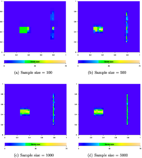
Figure 3: Density estimate for a mixture of uniform and “semi-Beta” using the posterior mean approach for an optional Pólya tree with the restriction of “alternate cutting.” The white blocks represent the density estimates falling outside of the intensity range plotted.

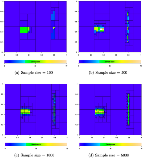
Figure 4: Density estimate for a mixture of uniform and “semi-Beta” by the hierarchical MAP method using an optional Pólya tree prior with the restriction of “alternate cutting.” The dark lines mark the representative partition learned from the method. The white blocks represent the density estimates falling outside of the intensity range plotted.

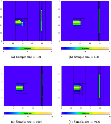
Figure 5: Density estimate for a mixture of uniform distribution and “semi-Beta” distribution by the hierarchical MAP method using an optional Pólya tree prior (with no restriction on division). The dark lines mark the representative partition learned from the method. The white blocks represent the density estimates falling outside of the intensity range plotted.

Pólya tree prior with the alternate cutting restriction (Figure 4); and (3) the hierarchical MAP method using an optional Pólya tree prior without any restriction on division (Figure 5). The last method does a much better job in capturing the underlying structure of the data, and thus requires a much smaller sample size to achieve decent estimates of the density.

Example 9 ((Bivariate normal)).

In our last example, we apply the hierarchical MAP method using an optional Pólya tree prior to samples from a bivariate normal distribution,

$$\operatorname{BN}\left(\pmatrix{0.6\cr 0.4},\pmatrix{0.1^{2}&0\cr 0&0.1^{2}}\right).$$

This example demonstrates how the posterior optional Pólya tree behaves in a multi-dimensional setting when the underlying distribution has smooth boundary (Figure 6).

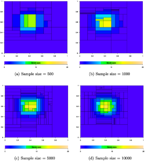
Figure 6: The hierarchical MAP method using an optional Pólya tree prior applied to samples from a bivariate normal distribution $\operatorname{BN}((0.4,0.6),0.1^{2}I)$.

Not surprisingly, the gradient or change in density is best captured when its direction is perpendicular to one of the coordinates (and thus is parallel to the other in the 2D case).

5 Concluding remarks

In this paper we established the existence and the theoretical properties of absolutely continuous probability measures obtained through the Introduction of randomized splitting variables and early stopping rules into a Pólya tree construction. For low-dimensional densities, it is possible to carry out exact computation to obtain posterior inferences based on this “optional Pólya tree” prior. A conceptually important feature of this approach is the ability to learn the partition underlying a piecewise constant density in a principled manner. Although the theory was motivated by applications in high-dimensional problems, at present exact computation is too demanding for such applications. The development of effective approximate computation should be a priority in future works.

Appendix

Here we describe an inductive procedure for computing the mean density function of an optional Pólya tree when the way to divide each elementary region is dichotomous and unique.

Let $A_{i}$ denote a level-$i$ elementary region and $(k_{1},k_{2},\ldots,k_{i})$ the sequence of left and right decisions to reach $A_{i}$ from the root node $\Omega$. That is, $A_{i}=\Omega_{k_{1}k_{2}\cdots k_{i}}$, where the $k$’s take values in {0, 1} indicating left and right, respectively. For simplicity, we let $A_{0}=\Omega$ represent the root node. Now for any point $x\in\Omega$, let $\{A_{i}\}$ be the sequence of nodes such that $x\in\bigcup_{i=0}^{\infty}A_{i}$. Assuming $\mu(A_{i})\downarrow 0$, the density of the mean distribution at $x$ is given by

$$\lim_{i\rightarrow\infty}EP(X\in A_{i})/\mu(A_{i}).$$

Therefore, to compute the mean density we just need a recipe for computing $EP(X\in A_{i})$ for any elementary region $A_{i}$. To achieve this goal, first let $A_{i}^{\prime}$ be the sibling of $A_{i}$ for all $i\geq 1$. That is,

$$A_{i}^{\prime}=\Omega_{k^{\prime}_{1}k^{\prime}_{2}\cdots k^{\prime}_{i}}\qquad\mbox{where $k^{\prime}_{j}=k_{j}$ for $j=1,2,\ldots,i-1$ and $k^{\prime}_{i}=1-k_{i}$.}$$

Next, for $i\geq 1$, let $\alpha_{i}$ and $\alpha_{i}^{\prime}$ be the Beta parameters for node $A_{i-1}$ associated with its two children $A_{i}$ and $A_{i}^{\prime}$. Also, for $i\geq 0$, let $\rho_{i}$ be the stopping probability of $A_{i}$, and $S_{i}$ the event that the tree has stopped growing on or before reaching node $A_{i}$. With this notation, we have for all $i\geq 1$,

$$EP(X\in A_{i}){\mathbf{1}}(S_{i})$$

$$\qquad=EP(X\in A_{i}){\mathbf{1}}(S_{i-1})+EP(X\in A_{i}){\mathbf{1}}(S_{i-1}^{c}){\mathbf{1}}(S_{i})$$

$$\qquad=\frac{\mu(A_{i})}{\mu(A_{i-1})}EP(X\in A_{i-1}){\mathbf{1}}(S_{i-1})$$

$$\qquad\quad{}+\frac{\alpha_{i}}{\alpha_{i}+\alpha_{i}^{\prime}}\rho_{i}EP(X\in A_{i-1}){\mathbf{1}}(S_{i-1}^{c})$$

and

$$EP(X\in A_{i}){\mathbf{1}}(S_{i}^{c}) = EP(X\in A^{i}){\mathbf{1}}(S_{i}^{c}){\mathbf{1}}(S_{i-1}^{c})$$

$$= \frac{\alpha_{i}}{\alpha_{i}+\alpha_{i}^{\prime}}(1-\rho_{i})EP(X\in A_{i-1}){\mathbf{1}}(S_{i-1}^{c}).$$

Now let $a_{i}=EP(X\in A_{i}){\mathbf{1}}(S_{i})$ and $b_{i}=EP(X\in A_{i}){\mathbf{1}}(S_{i}^{c})$, then the above equations can be rewritten as

$$\cases{\displaystyle a_{i}=\frac{\mu(A_{i})}{\mu(A_{i-1})}a_{i-1}+\frac{\alpha_{i}}{\alpha_{i}+\alpha_{i}^{\prime}}\rho_{i}b_{i-1},\cr\displaystyle b_{i}=\frac{\alpha_{i}}{\alpha_{i}+\alpha_{i}^{\prime}}(1-\rho_{i})b_{i-1},}$$ (4)

for all $i\geq 1$. Because $a_{o}=EP(X\in\Omega){\mathbf{1}}(S_{0})=P(S_{0})=\rho_{0}$, and $b_{0}=1-a_{0}=1-\rho_{0}$, we can apply (4) inductively to compute the $a_{i}$ and $b_{i}$ for all $A_{i}$’s. Because $EP(X\in A_{i})=a_{i}+b_{i}$, the mean density at $x$ is given by

$$\lim_{i\rightarrow\infty}EP(X\in A_{i})/\mu(A_{i})=\lim_{i\rightarrow\infty}(a_{i}+b_{i})/\mu(A_{i}).$$

References

- (1) Blackwell, D. (1973). Discreteness of Ferguson selections. Ann. Statist. 1 356–358. \MR0348905
- (2) Blackwell, D. and MacQueen, J. B. (1973). Ferguson distributions via Pólya urn schemes. Ann. Statist. 1 353–355. \MR0362614
- (3) Breiman, L., Friedman, J. H., Olshen, R. A. and Stone, C. J. (1984). Classification and Regression Trees. Wadsworth Advanced Books and Software, Belmont, CA. \MR0726392
- (4) Denison, D. G. T., Mallick, B. K. and Smith, A. F. M. (1998). A Bayesian CART algorithm. Biometrika 85 363–377. \MR1649118
- (5) Diaconis, P. and Freedman, D. (1986). On inconsistent Bayes estimates of location. Ann. Statist. 14 68–87. \MR0829556
- (6) Fabius, J. (1964). Asymptotic behavior of Bayes’ estimates. Ann. Math. Statist. 35 846–856. \MR0162325
- (7) Ferguson, T. S. (1973). A Bayesian analysis of some nonparametric problems. Ann. Statist. 1 209–230. \MR0350949
- (8) Ferguson, T. S. (1974). Prior distributions on spaces of probability measures. Ann. Statist. 2 615–629. \MR0438568
- (9) Freedman, D. A. (1963). On the asymptotic behavior of Bayes’ estimates in the discrete case. Ann. Math. Statist. 34 1386–1403. \MR0158483
- (10) Ghosh, J. K. and Ramamoorthi, R. V. (2003). Bayesian Nonparametrics. Springer, New York. \MR1992245
- (11) Hanson, T. E. (2006). Inference for mixtures of finite Pólya tree models. J. Amer. Statist. Assoc. 101 1548–1565. \MR2279479
- (12) Hutter, M. (2009). Exact nonparametric Bayesian inference on infinite trees. Technical Report 0903.5342. Available at http://arxiv.org/abs/0903.5342.
- (13) Kraft, C. H. (1964). A class of distribution function processes which have derivatives. J. Appl. Probab. 1 385–388. \MR0171296
- (14) Lavine, M. (1992). Some aspects of Pólya tree distributions for statistical modelling. Ann. Statist. 20 1222–1235. \MR1186248
- (15) Lavine, M. (1994). More aspects of Pólya tree distributions for statistical modelling. Ann. Statist. 22 1161–1176. \MR1311970
- (16) Lo, A. Y. (1984). On a class of Bayesian nonparametric estimates. I. Density estimates. Ann. Statist. 12 351–357. \MR0733519
- (17) Mauldin, R. D., Sudderth, W. D. and Williams, S. C. (1992). Pólya trees and random distributions. Ann. Statist. 20 1203–1221. \MR1186247
- (18) Nieto-Barajas, L. E. and Müller, P. (2009). Unpublished manuscript.
- (19) Paddock, S. M., Ruggeri, F., Lavine, M. and West, M. (2003). Randomized Polya tree models for nonparametric Bayesian inference. Statist. Sinica 13 443–460. \MR1977736
- (20) Schwartz, L. (1965). On Bayes procedures. Z. Wahrsch. Verw. Gebiete 4 10–26. \MR0184378