Lipschitz metric for the Camassa–Holm equation on the line

Abstract.

We study stability of solutions of the Cauchy problem on the line for the Camassa–Holm equation $u_{t}-u_{xxt}+3uu_{x}-2u_{x}u_{xx}-uu_{xxx}=0$ with initial data $u_{0}$. In particular, we derive a new Lipschitz metric $d_{\mathcal{D}}$ with the property that for two solutions $u$ and $v$ of the equation we have $d_{\mathcal{D}}(u(t),v(t))\leq e^{Ct}d_{\mathcal{D}}(u_{0},v_{0})$. The relationship between this metric and the usual norms in $H^{1}$ and $L^{\infty}$ is clarified. The method extends to the generalized hyperelastic-rod equation $u_{t}-u_{xxt}+f(u)_{x}-f(u)_{xxx}+(g(u)+\frac{1}{2}f^{\prime\prime}(u)(u_{x})^{2})_{x}=0$ (for $f$ without inflection points).

1. Introduction

The Cauchy problem for the Camassa–Holm (CH) equation [3, 4],

(1.1) $$u_{t}-u_{txx}+\kappa u_{x}+3uu_{x}-2u_{x}u_{xx}-uu_{xxx}=0,$$

where $\kappa\in\mathbb{R}$ is a constant, has attracted much attention due to the fact that it serves as a model for shallow water waves [8] and its rich mathematical structure. For example, it has a bi-Hamiltonian structure, infinitely many conserved quantities and blow-up phenomena have been studied, see, e.g., [5], [6], and [7].

We here focus on the construction of the Lipschitz metric for the semigroup of conservative solutions on the real line. This problem has been recently considered by Grunert, Holden, and Raynaud [12] in the periodic case, and here we want to present how the approach used there has to be modified in the non-periodic case.

For simplicity, we will only discuss the case $\kappa=0$, that is,

(1.2) $$u_{t}-u_{txx}+3uu_{x}-2u_{x}u_{xx}-uu_{xxx}=0,$$

and from now on we refer to (1.2) as the CH equation. However, the approach presented here can also handle the generalized hyperelastic-rod equation, see Remark 2.9. In particular, it includes the case with nonzero $\kappa$. The generalized hyperelastic-rod equation has been introduced in [15]. It is given by

(1.3) $$u_{t}-u_{xxt}+f(u)_{x}-f(u)_{xxx}+(g(u)+\frac{1}{2}f^{\prime\prime}(u)(u_{x})^{2})_{x}=0$$

where $f$ and $g$ are smooth functions. With $f(u)=\frac{u^{2}}{2}$ and $g(u)=\kappa u+u^{2}$, we recover (1.1) for any $\kappa$. With $f(u)=\frac{\gamma u^{2}}{2}$ and $g(u)=\frac{3-\gamma}{2}u^{2}$, we obtain the hyperelastic-rod wave equation:

$$u_{t}-u_{txx}+3uu_{x}-\gamma(2u_{x}u_{xx}+uu_{xxx})=0,$$

which has been introduced by Dai [9, 10, 11].

Equation (1.2) can be rewritten as the following system

(1.4) $$u_{t}+uu_{x}+P_{x} =0,$$

(1.5) $$P-P_{xx}=u^{2}+ \frac{1}{2}u_{x}^{2},$$

where we choose $u$ to be an element of $H^{1}(\mathbb{R})$. The $H^{1}$ norm is preserved as

(1.6) $$\frac{d}{dt}\left\|u(t)\right\|_{H^{1}(\mathbb{R})}^{2}=\frac{d}{dt}\int_{\mathbb{R}}(u^{2}+u_{x}^{2})dx=0,$$

for any smooth solution $u$. However, even for smooth initial data, the solution may break down in finite time. In this case, the solution experiences wave breaking ([4, 5]): The solution remains bounded while, at some point, the spatial derivative $u_{x}$ tends to $-\infty$. This phenomenon can be nicely illustrated by the so called multipeakon solutions. These are solutions of the form

(1.7) $$u(t,x)=\sum_{i=1}^{n}p_{i}(t)e^{-\left|x-q_{i}(t)\right|}.$$

Let us consider the case with $n=2$ and one peakon $p_{1}(0)>0$ (moving to the right) and one antipeakon $p_{2}(0)<0$ (moving to the left). In the symmetric case ($p_{1}(0)=-p_{2}(0)$ and $q_{1}(0)=-q_{2}(0)<0$) the solution $u$ will vanish pointwise at the collision time $t^{*}$ when $q_{1}(t^{*})=q_{2}(t^{*})$, that is, $u(t^{*},x)=0$ for all $x\in\mathbb{R}$. At time $t=t^{*}$, the whole energy is concentrated at the origin, and we have $\lim_{t\to t^{*}}(u^{2}+u_{x}^{2})\,dx=\left\|u_{0}\right\|_{H^{1}}\delta$, with $\delta$ denoting the Dirac delta distribution at the origin. In general we have two possibilities to continue the solution beyond wave breaking, namely to set $u$ identically equal to zero for $t>t^{\star}$, which is called a dissipative solution, or to let the peakons pass through each other, which is called a conservative solution and which is depicted in Figure 1. We are interested in the latter case, for which solutions have been studied by Bressan and Constantin [1] and Holden and Raynaud [13, 14]. Since the $H^{1}$-norm is preserved, the space $H^{1}$ appears as a natural space for the semigroup of solutions. However, the previous multipeakon example reveals the opposite. Indeed, $u(t^{*},x)=0$ for all $x\in\mathbb{R}$. Thus, the trivial solution $\bar{u}$, that is, $\bar{u}(t,x)=0$ for all $t,x\in\mathbb{R}$, which is also a conservative solution, coincides with $u$ at $t=t^{*}$. To define a semigroup of conservative solutions, we therefore need more information about the solution than just its pointwise values, for instance, the amount and location of the energy which concentrates on sets of zero measure. This justifies the introduction of the set $\mathcal{D}$ of Eulerian coordinates, see Definition 4.1, for which a semigroup can be constructed [13].

Furthermore, the $H^{1}$ norm is not well suited to establish a stability result. Consider, e.g., the sequence of multipeakons $u^{\varepsilon}$ defined as $u^{\varepsilon}(t,x)=u(t-\varepsilon,x)$, see Figure 1. Then, assuming that $\left\|u(0)\right\|_{H^{1}(\mathbb{R})}=1$, we have

$$\lim_{\varepsilon\to 0}\left\|u(0)-u^{\varepsilon}(0)\right\|_{H^{1}(\mathbb{R})}=0,\quad\text{and}\quad\left\|u(t^{\star})-u^{\varepsilon}(t^{\star})\right\|_{H^{1}(\mathbb{R})}=\left\|u^{\varepsilon}(t^{\star})\right\|_{H^{1}(\mathbb{R})}=1,$$

so that the flow is clearly discontinuous with respect to the $H^{1}$ norm.

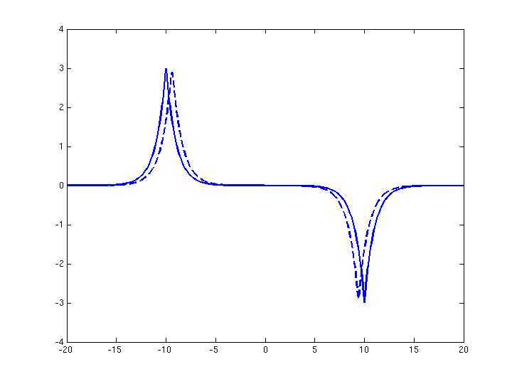
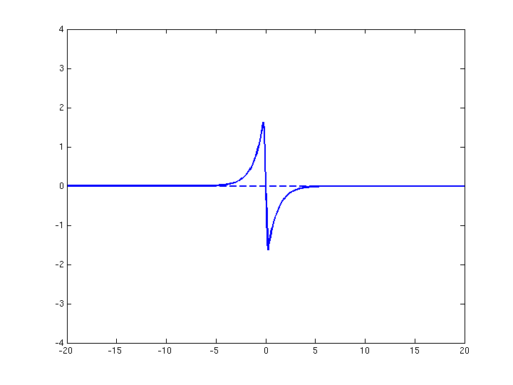
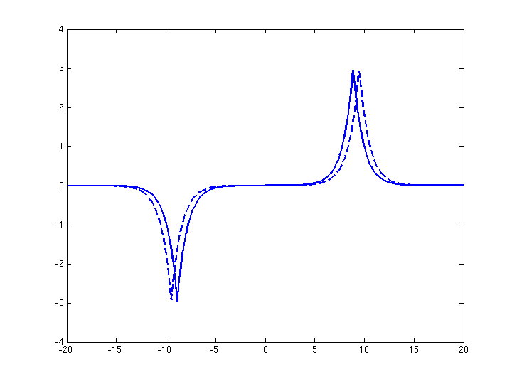
Figure 1. The dashed curve depicts the antisymmetric multipeakon solution $u(t,x)$, which vanishes at $t^{*}$, for $t=0$ (left) and $t=t^{*}$ (middle) and $t=2t^{*}$ (right). The solid curve depicts the multipeakon solution given by $u^{\varepsilon}(t,x)=u(t-\varepsilon,x)$ for some small $\varepsilon>0$ (the CH equation is invariant with respect to time translation).

The aim of this article is to present a metric for which the semigroup of conservative solutions on the line is Lipschitz continuous. A more extensive discussion about Lipschitz continuity with examples from ordinary differential equations, can be found in [2]. A detailed presentation for the Camassa–Holm equation in the periodic case is presented in [12], thus we here focus on explaining the differences between the periodic case and the decaying case. However, we first present the general construction.

The construction of the metric is closely connected to the construction of the semigroup itself. Let us outline this construction. We rewrite the CH equation in Lagrangian coordinates and obtain a semilinear system of ordinary differential equations: Let $u(t,x)$ denote the solution and $y(t,\xi)$ the corresponding characteristics, thus $y_{t}(t,\xi)=u(t,y(t,\xi))$. Then our new variables are $y(t,\xi)$, as well as

(1.8) $$U(t,\xi)=u(t,y(t,\xi)),\quad H(t,\xi)=\int_{-\infty}^{y(t,\xi)}(u^{2}+u_{x}^{2})dx,$$

where $U$ corresponds to the Lagrangian velocity while $H$ can be interpreted as the Lagrangian cumulative energy distribution. The time evolution for any $X=(y,U,H)$ is described by

(1.9) $$y_{t} =U,$$

$$U_{t} =-Q,$$

$$H_{t} =U^{3}-2PU,$$

where

(1.10) $$P(t,\xi)=\frac{1}{4}\int_{\mathbb{R}}\exp(-|y(t,\xi)-y(t,\eta)|)(U^{2}y_{\xi}+H_{\xi})(t,\eta)d\eta,$$

and

(1.11) $$Q(t,\xi)=-\frac{1}{4}\int_{\mathbb{R}}\mathop{\rm sign}(y(t,\xi)-y(t,\eta))\exp(-|y(t,\xi)-y(t,\eta)|)(U^{2}y_{\xi}+H_{\xi})(t,\eta)d\eta.$$

This system is well-posed as a locally Lipschitz system of ordinary differential equations in a Banach space, and we can define a semigroup of solution which we denote $S_{t}$. From standard theory for ordinary differential equations we know that $S_{t}$ is locally Lipschitz continuous, that is, given $T$ and $M$,

(1.12) $$\left\|S_{t}(X_{\alpha})-S_{t}(X_{\beta})\right\|\leq C_{M,T}\left\|X_{\alpha}-X_{\beta}\right\|$$

for any $t\in[0,T]$, $X_{\alpha},X_{\beta}\in B_{M}=\{X\ |\ \left\|X\right\|\leq M\}$ and where the constant $C_{M,T}$ depends only on $M$ and $T$.

The mapping from Lagrangian to Eulerian coordinates is surjective but not bijective. The discrepancy between the two sets of coordinates is due to the freedom of relabeling in Lagrangian coordinates. The relabeling functions form a group, which we denote $G$, and which basically consists of the diffeomorphisms of the line with some additional assumptions (see Definition 2.3). Given $X=(y,U,H)$, the element $X\circ f=(y\circ f,U\circ f,H\circ f)$ is the relabeled version of $X$ by the relabeling function $f\in G$. Using the fact that the semigroup $S_{t}$ is equivariant with respect to relabeling, that is,

(1.13) $$S_{t}(X\circ f)=S_{t}(X)\circ f,$$

we can construct a semigroup of solutions on equivalence classes from $S_{t}$. Finally, after establishing the existence of a bijection between the Eulerian coordinates and the equivalence classes in Lagrangian coordinates, we can transport the semigroup of solutions defined on equivalence classes and construct a semigroup, which we denote $T_{t}$, of conservative solutions in $\mathcal{D}$.

We want to find a metric which makes $T_{t}$ Lipschitz continuous. For that purpose, we introduce a pseudometric in Lagrangian coordinates which does not distinguish between elements of the same equivalence class and which, at the same time, leaves the semigroup $S_{t}$ locally Lipschitz continuous. This strategy has been used in [2] for the Hunter–Saxton equation and in [12] for the Camassa–Holm equation in the periodic case. In [2], the pseudometric is defined by using ideas from Riemannian geometry. Here, we follow the approach of [12] and first introduce a pseudosemimetric which also identifies elements of the same equivalence class and leaves $S_{t}$ Lipschitz continuous. A natural choice, which was applied in [12], is to consider the pseudometric $\tilde{J}$ defined as

(1.14) $$\tilde{J}(X_{\alpha},X_{\beta})=\inf_{f,g\in G}\left\|X_{\alpha}\circ f-X_{\beta}\circ g\right\|.$$

The pseudometric $\tilde{J}$ identifies elements of the same equivalence class, as $\tilde{J}(X,X\circ f)=0$. Moreover, it is invariant with respect to relabeling, that is, $\tilde{J}(X_{\alpha}\circ f,X_{\beta}\circ g)=\tilde{J}(X_{\alpha},X_{\beta})$ for any $f,g\in G$. It remains to prove that the pseudosemimetric makes the semigroup $S_{t}$ locally Lipschitz, that is, given $M$ and $T$, there exists a constant $C$ depending on $M$ and $T$ such that

(1.15) $$\tilde{J}(S_{t}X_{\alpha},S_{t}X_{\beta})\leq C\tilde{J}(X_{\alpha},X_{\beta}),$$

for all $t\in[0,T]$ and $X_{\alpha},X_{\beta}\in B_{M}$. The proof follows almost directly from the stability and equivariance of $S_{t}$. We outline it here. For every $\varepsilon>0$, there exist $f,g\in G$ such that $\tilde{J}(X_{\alpha},X_{\beta})\geq\left\|X_{\alpha}\circ f-X_{\beta}\circ g\right\|-\varepsilon$ and we get

(1.16a) $$\tilde{J}(S_{t}X_{\alpha},S_{t}X_{\beta}) \leq\left\|S_{t}(X_{\alpha})\circ f-S_{t}(X_{\beta})\circ g\right\|$$

(1.16b) $$=\left\|S_{t}(X_{\alpha}\circ f)-S_{t}(X_{\beta}\circ g)\right\| S_{t}$$ (as is equivariant)

(1.16c) $$\leq C_{M}\left\|X_{\alpha}\circ f-X_{\beta}\circ g\right\|$$ (by (1.12))

(1.16d) $$\leq C_{M}(\tilde{J}(X_{\alpha},X_{\beta})+\varepsilon)$$

and (1.15) follows by letting $\varepsilon$ tend to zero. However, the use of the Lipschitz stability of $S_{t}$ (1.12) relies on bounds on $\left\|X_{\alpha}\circ f\right\|$ and $\left\|X_{\beta}\circ g\right\|$ that are unavailable. The problem is that the norm $\left\|\,\cdot\,\right\|$ of the Banach space is not invariant with respect to relabeling and therefore, since $f$ and $g$ are a priori arbitrary, we cannot obtain any bound depending on $M$ for $\left\|X_{\alpha}\circ f\right\|$ and $\left\|X_{\beta}\circ g\right\|$. This motivates the introduction in this paper of the pseudosemimetric $J$ defined as

(1.17) $$J(X_{\alpha},X_{\beta})=\inf_{f_{1},f_{2}\in G}\big{(}\left\|X_{\alpha}\circ f_{1}-X_{\beta}\right\|+\left\|X_{\alpha}-X_{\beta}\circ f_{2}\right\|\big{)}.$$

As expected, the pseudosemimetric $J$ identifies equivalence classes (we have $J(X,X\circ f)=0$) but we lose the nice relabeling invariance property. At the same time, this definition of $J$ implies some implicit restrictions on the diffeomorphisms $f_{1}$ and $f_{2}$ which allow us to bound the relabeled versions $\left\|X_{\alpha}\circ f_{1}\right\|$ and $\left\|X_{\beta}\circ f_{2}\right\|$ so that the approach sketched in (1.16) can be carried out.

It remains to explain why, in the periodic case [12], we could use the definition of $\tilde{J}$, which is a more natural definition and moreover simplifies the proofs. In the periodic case (we take the period equal to one), the stability of the semigroup $S_{t}$ is established in the space $W^{1,1}([0,1])$ equipped with the norm

(1.18) $$\left\|U\right\|_{W^{1,1}([0,1])}=\left\|U\right\|_{L^{\infty}([0,1])}+\left\|U_{\xi}\right\|_{L^{1}([0,1])}.$$

Note that, in order to keep these formal explanations as simple as possible, we just consider the second component of $X=(y,U,H)$. Since $\left\|U\circ f\right\|_{L^{\infty}}=\left\|U\right\|_{L^{\infty}}$ and

$$\left\|U\circ f\right\|_{L^{1}}=\int_{0}^{1}U\circ ff_{\xi}\,d\xi=\left\|U\right\|_{L^{1}}$$

we have $\left\|U\circ f\right\|_{W^{1,1}}=\left\|U\right\|_{W^{1,1}}$, for any $f\in G$, so that the norm defined in (1.18) is relabeling invariant. Now, if the norm of the Banach space is relabeling invariant, we have

(1.19) $$\tilde{J}(X_{\alpha},X_{\beta})\leq J(X_{\alpha},X_{\beta})\leq 2\tilde{J}(X_{\alpha},X_{\beta}),$$

and the pseudosemimetrics $J$ and $\tilde{J}$ are equivalent. However, the natural Banach space for $U$ is not $W^{1,1}([0,1])$ but $W^{1,2}([0,1])=H^{1}([0,1])$. In the periodic case, it is not an issue as $H^{1}([0,1])\subset W^{1,1}([0,1])$ but the corresponding embedding does not hold in the case of the real line. This also shows that the approach that we present here for the real line can also be used in the periodic case and that the novelty in this article is that we handle a norm which is not relabeling invariant.

The final step consists of deriving a pseudometric from the pseudosemimetric $J$. This can be achieved by the following general construction: Let

$$d(X_{\alpha},X_{\beta})=\inf\sum_{i=1}^{N}J(X_{n-1},X_{n}),$$

where the infimum is taken over all finite sequences $\{X_{n}\}_{n=0}^{N}$ with $X_{0}=X_{\alpha}$ and $X_{N}=X_{\beta}$. The pseudometric $d$ inherits the Lipschitz stability property (1.15) from $J$. Finally, identifying elements belonging to the same equivalence class, the pseudometric $d$ turns into a metric on the set of equivalence classes. By bijection, it yields a metric in $\mathcal{D}$ which makes the semigroup of conservative solutions Lipschitz continuous.

In the last section, Section 5, we compare this new metric with the usual norms in $H^{1}$ and $L^{\infty}$.

2. Semigroup of solutions in Lagrangian coordinates

In this section, we recall from [13] the construction of the semigroup in Lagrangian coordinates. The Camassa–Holm equation reads

(2.1) $$u_{t}-u_{xxt}+3uu_{x}-2u_{x}u_{xx}-uu_{xxx}=0,$$

and can be rewritten as the following system

(2.2) $$u_{t}+uu_{x}+P_{x}=0,$$

(2.3) $$P-P_{xx}=u^{2}+\frac{1}{2}u_{x}^{2}.$$

Next, we rewrite the equation in Lagrangian coordinates. Therefore we introduce the characteristics

(2.4) $$y_{t}(t,\xi)=u(t,y(t,\xi)).$$

The Lagrangian velocity $U$ reads

(2.5) $$U(t,\xi)=u(t,y(t,\xi)).$$

We define the Lagrangian cumulative energy as

(2.6) $$H(t,\xi)=\int_{-\infty}^{y(t,\xi)}(u^{2}+u_{x}^{2})dx.$$

As an immediate consequence of the definition of the characteristics we obtain

(2.7) $$U_{t}(t,\xi)=u_{t}(t,y)+y_{t}(t,\xi)u_{x}(t,y)=-P_{x}\circ y(t,\xi).$$

The last term can be expressed uniquely in terms of $y$, $U$, and $H$. From (2.3) we obtain the following explicit expression for $P$,

(2.8) $$P(t,x)=\frac{1}{2}\int_{\mathbb{R}}e^{-|x-z|}\Big{(}u^{2}(t,z)+\frac{1}{2}u_{x}^{2}(t,z)\Big{)}dz.$$

Setting $Q(t,\xi)=P_{x}(t,y(t,\xi))$ and writing $P(t,\xi)=P(t,y(t,\xi))$, we obtain

(2.9) $$P(t,\xi)=\frac{1}{4}\int_{\mathbb{R}}\exp(-|y(t,\xi)-y(t,\eta)|)(U^{2}y_{\xi}+H_{\xi})(t,\eta)d\eta,$$

and

(2.10) $$Q(t,\xi)=-\frac{1}{4}\int_{\mathbb{R}}\mathop{\rm sign}(y(t,\xi)-y(t,\eta))\exp(-|y(t,\xi)-y(t,\eta)|)(U^{2}y_{\xi}+H_{\xi})(t,\eta)d\eta.$$

Moreover we introduce another variable $\zeta(t,\xi)=y(t,\xi)-\xi$. Thus we have derived a new system of equations, which is up to that point only formally equivalent to the Camassa–Holm equation:

(2.11) $$\zeta_{t} =U,$$

$$U_{t} =-Q,$$

$$H_{t} =U^{3}-2PU.$$

Let $V$ be the Banach space defined by

$$V=\{f\in C_{b}(\mathbb{R})\ |\ f_{\xi}\in L^{2}\}$$

where $C_{b}(\mathbb{R})=C(\mathbb{R})\cap L^{\infty}$ and the norm of $V$ is given by $\left\|f\right\|_{V}=\left\|f\right\|_{L^{\infty}}+\left\|f_{\xi}\right\|_{L^{2}}$. Of course $H^{1}\subset V$ but the converse is not true as $V$ contains functions that do not vanish at infinity. We will employ the Banach space $E$ defined by

$$E=V\times H^{1}\times V$$

with the following norm $\left\|X\right\|=\left\|\zeta\right\|_{V}+\left\|U\right\|_{H^{1}(\mathbb{R})}+\left\|H\right\|_{V}$ for any $X=(\zeta,U,H)\in E$.

Definition 2.1.

The set $\mathcal{G}$ is composed of all $(\zeta,U,H)\in E$ such that

(2.12a) $$(\zeta,U,H)\in\left[W^{1,\infty}\right]^{3},$$

(2.12b) $$y_{\xi}\geq 0,H_{\xi}\geq 0,y_{\xi}+H_{\xi}>0\text{ almost everywhere, and }\lim_{\xi\rightarrow-\infty}H(\xi)=0,$$

(2.12c) $$y_{\xi}H_{\xi}=y_{\xi}^{2}U^{2}+U_{\xi}^{2}\text{ almost everywhere},$$

where we denote $y(\xi)=\zeta(\xi)+\xi$.

Given a constant $M>0$, we denote by $B_{M}$ the ball

(2.13) $$B_{M}=\{X\in E\ |\ \left\|X\right\|\leq M\}.$$

Theorem 2.2.

For any $\bar{X}=(\bar{y},\bar{U},\bar{H})\in\mathcal{G}$, the system (2.11) admits a unique global solution $X(t)=(y(t),U(t),H(t))$ in $C^{1}(\mathbb{R}_{+},E)$ with initial data $\bar{X}=(\bar{y},\bar{U},\bar{H})$. We have $X(t)\in\mathcal{G}$ for all times. If we equip $\mathcal{G}$ with the topology induced by the $E$-norm, then the mapping $S\colon\mathcal{G}\times\mathbb{R}_{+}\to\mathcal{G}$ defined by

$$S_{t}(\bar{X})=X(t)$$

is a continuous semigroup. More precisely, given $M>0$ and $T>0$, there exists a constant $C_{M}$ which depends only on $M$ and $T$ such that, for any two elements $X_{\alpha},X_{\beta}\in\mathcal{G}\cap B_{M}$, we have

(2.14) $$\left\|S_{t}X_{\alpha}-S_{t}X_{\beta}\right\|\leq C_{M}\left\|X_{\alpha}-X_{\beta}\right\|$$

for any $t\in[0,T]$.

Proof.

We have

$$X_{t}=F(X)$$

where $F$ is locally Lipschitz (see proof [13, Theorem 2.3]). It implies, by Gronwall’s lemma, that we have

$$\left\|S_{t}(X_{\alpha})-S_{t}(X_{\beta})\right\|\leq C\left\|X_{\alpha}-X_{\beta}\right\|$$

for $t\in[0,T]$, where the constant $C$ only depends on $\sup_{t\in[0,T]}\left\|S_{t}(X_{\alpha})\right\|$ and $\sup_{t\in[0,T]}\left\|S_{t}(X_{\beta})\right\|$. In [13, Theorem 2.8] it is proved that $\sup_{t\in[0,T]}\left\|S_{t}(X_{\alpha})\right\|$ only depends of $\left\|X_{\alpha}\right\|$ and $T$, and thus on $M$ and $T$. ∎

Definition 2.3.

We denote by $G$ the subgroup of the group of homeomorphisms from $\mathbb{R}$ to $\mathbb{R}$ such that

(2.15a) $$f-\operatorname{Id}\text{ and }f^{-1}-\operatorname{Id} \text{ both belong to }W^{1,\infty}(\mathbb{R}),$$

(2.15b) $$f_{\xi}-1 \text{ belongs to }L^{2}(\mathbb{R}),$$

where $\operatorname{Id}$ denotes the identity function. Given $\kappa>0$, we denote by $G_{\kappa}$ the subset $G_{\kappa}$ of $G$ defined by

$$G_{\kappa}=\{f\in G\ |\ \left\|f-\operatorname{Id}\right\|_{{W^{1,\infty}(\mathbb{R})}}+\left\|f^{-1}-\operatorname{Id}\right\|_{{W^{1,\infty}(\mathbb{R})}}\leq\kappa\}.$$

The subsets $G_{\kappa}$ do not possess the group structure of $G$. The next lemma provides a useful characterization of $G_{\kappa}$.

Lemma 2.4 ([13, Lemma 3.2]).

Let $\kappa\geq 0$. If $f$ belongs to $G_{\kappa}$, then $1/(1+\kappa)\leq f_{\xi}\leq 1+\kappa$ almost everywhere. Conversely, if $f$ is absolutely continuous, $f-\operatorname{Id}\in{W^{1,\infty}(\mathbb{R})}$, $f$ satisfies (2.15b) and there exists $c\geq 1$ such that $1/c\leq f_{\xi}\leq c$ almost everywhere, then $f\in G_{\kappa}$ for some $\kappa$ depending only on $c$ and $\left\|f-\operatorname{Id}\right\|_{{W^{1,\infty}(\mathbb{R})}}$.

We define the subsets $\mathcal{F}_{\kappa}$ and $\mathcal{F}$ of $\mathcal{G}$ as follows

$$\mathcal{F}_{\kappa}=\{X=(y,U,H)\in\mathcal{G}\ |\ y+H\in G_{\kappa}\},$$

and

$$\mathcal{F}=\{X=(y,U,H)\in\mathcal{G}\ |\ y+H\in G\}.$$

For $\kappa=0$, $G_{0}=\{\operatorname{Id}\}$. As we shall see, the space $\mathcal{F}_{0}$ will play a special role. These sets are relevant only because they are preserved by the governing equation (2.11) as the next lemma shows. In particular, while the mapping $\xi\mapsto y(t,\xi)$ may not be a diffeomorphism for some time $t$, the mapping $\xi\mapsto y(t,\xi)+H(t,\xi)$ remains a diffeomorphism for all times $t$.

Lemma 2.5.

The space $\mathcal{F}$ is preserved by the governing equation (2.11). More precisely, given $\kappa,T\geq 0$, there exists $\kappa^{\prime}$ which only depends on $T$, $\kappa$ and $\left\|\bar{X}\right\|$ such that

$$S_{t}(\bar{X})\in\mathcal{F}_{\kappa^{\prime}}$$

for any $\bar{X}\in\mathcal{F}_{\kappa}$.

Proof.

Let $\bar{X}=(\bar{y},\bar{U},\bar{H})\in\mathcal{F}_{\kappa}$, we denote by $X(t)=(y(t),U(t),H(t))$ the solution of (2.11) with initial data $\bar{X}$ and set $h(t,\xi)=y(t,\xi)+H(t,\xi)$, $\bar{h}(\xi)=\bar{y}(\xi)+\bar{H}(\xi)$. By definition, we have $\bar{h}\in G_{\kappa}$ and, from Lemma 2.4, $1/c\leq\bar{h}_{\xi}\leq c$ almost everywhere, for some constant $c>1$ depending only on $\kappa$. We consider a fixed $\xi$ and drop it in the notation. Applying Gronwall’s inequality backward in time to (2.11) we obtain

(2.16) $$|y_{\xi}(0)|+|H_{\xi}(0)|+|U_{\xi}(0)|\leq\mathrm{e}^{CT}(|y_{\xi}(t)|+|H_{\xi}(t)|+|U_{\xi}(t)|),$$

for some constant $C$ which depends on $\left\|X(t)\right\|_{C([0,T],E)}$, which itself depends only on $\left\|\bar{X}\right\|$ and $T$. From (2.12c), we have

(2.17) $$|U_{\xi}(t)|\leq\sqrt{y_{\xi}(t)H_{\xi}(t)}\leq\frac{1}{2}(y_{\xi}(t)+H_{\xi}(t)).$$

Hence, since $y_{\xi}$ and $H_{\xi}$ are positive, (2.16) gives us

(2.18) $$\frac{1}{c}\leq\bar{y}_{\xi}+\bar{H}_{\xi}\leq\frac{3}{2}\mathrm{e}^{CT}(y_{\xi}(t)+H_{\xi}(t)),$$

and $h_{\xi}(t)=y_{\xi}(t)+H_{\xi}(t)\geq\frac{2}{3c}\mathrm{e}^{-CT}$. Similarly, by applying Gronwall’s lemma forward in time, we obtain $y_{\xi}(t)+H_{\xi}(t)\leq\frac{3}{2}c\,\mathrm{e}^{CT}$. We have $\left\|(y+H)(t)-\xi\right\|_{L^{\infty}(\mathbb{R})}\leq\left\|X(t)\right\|_{C([0,T],E)}\leq C$ and $\left\|y_{\xi}+H_{\xi}-1\right\|_{L^{2}}\leq\left\|\zeta_{\xi}\right\|_{L^{2}}+\left\|H_{\xi}\right\|_{L^{2}}\leq C$ for another constant $C$ which only depends on $\left\|\bar{X}\right\|$ and $T$. Hence, applying Lemma 2.4, we obtain that $y(t,\,\cdot\,)+H(t,\,\cdot\,)\in G_{\kappa^{\prime}}$ and therefore $X(t)\in F_{\kappa^{\prime}}$ for some $\kappa^{\prime}$ depending only on $\kappa$, $T$, and $\left\|\bar{X}\right\|$. ∎

For the sake of simplicity, for any $X=(y,U,H)\in\mathcal{F}$ and any function $f\in G$, we denote $(y\circ f,U\circ f,H\circ f)$ by $X\circ f$. This operation corresponds to relabeling.

Definition 2.6.

We denote by $\Pi(X)$ the projection of $\mathcal{F}$ into $\mathcal{F}_{0}$ defined as

$$\Pi(X)=X\circ(y+H)^{-1}$$

for any $X=(y,U,H)\in\mathcal{F}$.

The element $\Pi(X)$ is the unique relabeled version of $X$ that belongs to $\mathcal{F}_{0}$.

Lemma 2.7.

The mapping $S_{t}$ is equivariant, that is,

$$S_{t}(X\circ f)=S_{t}(X)\circ f.$$

This follows from the governing equation and the equivariance of the mappings $X\mapsto P(X)$ and $X\mapsto Q(X)$, where $P$ and $Q$ are defined in (2.9) and (2.10), see [13] for more details. From this lemma we get that

(2.19) $$\Pi\circ S_{t}\circ\Pi=\Pi\circ S_{t}.$$

Definition 2.8.

We define the semigroup $\bar{S}_{t}$ on $\mathcal{F}_{0}$ as

$$\bar{S}_{t}=\Pi\circ S_{t}.$$

The semigroup property of $\bar{S}_{t}$ follows from (2.19). From [13], we know that $\bar{S}_{t}$ is continuous with respect to the norm of $E$. It follows basically from the continuity of the mapping $\Pi$, but $\Pi$ is not Lipschitz continuous and the goal of the next section is to find a metric that makes $\bar{S}_{t}$ Lipschitz continuous.

Remark 2.9.

The details of the construction of the semigroup of solutions in Lagrangian coordinates for the generalized hyperelastic-rod equation (1.3) is given in [15]. The construction is based on a reformulation of the equation in Lagrangian coordinates which leads to a semilinear system of equations, similar to (2.11) for the Camassa–Holm equation. In the case of the generalized hyperelastic-rod equation, the equation can be rewritten as

(2.20) $$\left\{\begin{aligned} \zeta_{t}&=f^{\prime}(U),\\ U_{t}&=-Q,\\ H_{t}&=G(U)-2PU,\end{aligned}\right.$$

where $G(v)$ is given by

(2.21) $$G(v)=\int_{0}^{v}(2g(z)+f^{\prime\prime}(z)z^{2})\,dz,$$

and

(2.22) $$Q(t,\xi)=-\frac{1}{2}\int_{\mathbb{R}}\mathop{\rm sign}(\xi-\eta)\exp\big{(}-\mathop{\rm sign}(\xi-\eta)(y(\xi)-y(\eta))\big{)}\\ \times\Big{(}\big{(}g(U)-\frac{1}{2}f^{\prime\prime}(U)U^{2}\big{)}y_{\xi}+\frac{1}{2}f^{\prime\prime}(U)H_{\xi}\Big{)}(\eta)\,d\eta,$$

(2.23) $$P(t,\xi)=\frac{1}{2}\int_{\mathbb{R}}\exp\big{(}-\mathop{\rm sign}(\xi-\eta)(y(\xi)-y(\eta))\big{)}\\ \times\Big{(}\big{(}g(U)-\frac{1}{2}f^{\prime\prime}(U)U^{2}\big{)}y_{\xi}+\frac{1}{2}f^{\prime\prime}(U)H_{\xi}\Big{)}(\eta)\,d\eta.$$

Section 2 outlines the construction of the semigroup of solutions in Lagrangian coordinates. The construction of the metric in Eulerian coordinates, which is given in the following sections, relies basically on two fundamental results of this section: The Lipschitz stability of the semigroup of solution in Lagrangian coordinates (Theorem 2.2) and the equivariance of the semigroup (Lemma 2.7). The same results hold for the generalized hyperelastic-rod equation, see [15, Theorem 2.8 and Theorem 3.6] so that it is possible to define a Lipschitz stable metric for this equation in the same way as we do it for the CH equation.

3. Lipschitz metric for the semigroup $\bar{S}_{t}$

Definition 3.1.

Let $X_{\alpha},X_{\beta}\in\mathcal{F}$, we define $J(X_{\alpha},X_{\beta})$ as

(3.1) $$J(X_{\alpha},X_{\beta})=\inf_{f_{1},f_{2}\in G}\big{(}\left\|X_{\alpha}\circ f_{1}-X_{\beta}\right\|+\left\|X_{\alpha}-X_{\beta}\circ f_{2}\right\|\big{)}.$$

The mapping $J$ is symmetric. Moreover, if $X_{\alpha}$ and $X_{\beta}$ are equivalent, then $J(X_{\alpha},X_{\beta})=0$. Our goal is to create a distance between equivalence classes, and that is the reason why we introduce the pseudosemimetric $\tilde{J}$ as follows in the periodic case ([12]).

Definition 3.2.

Let $X_{\alpha},X_{\beta}\in\mathcal{F}$, we define $\tilde{J}(X_{\alpha},X_{\beta})$ as

$$\tilde{J}(X_{\alpha},X_{\beta})=\inf_{f,g\in G}\left\|X_{\alpha}\circ f-X_{\beta}\circ g\right\|.$$

The pseudosemimetric $\tilde{J}$ is relabeling invariant, that is, $\tilde{J}(X_{\alpha}\circ f,X_{\beta}\circ g)=\tilde{J}(X_{\alpha},X_{\beta})$. With Definition 3.1, we lose this important property. However, Definition 3.1 allows us to obtain estimates that cannot be obtained by Definition 3.2, see the proof of Theorem 3.10. In addition, it turns out that we do not actually need the relabeling invariance property to hold strictly and the estimates contained in the following lemma are enough for our purpose.

Lemma 3.3.

Given $X_{\alpha},X_{\beta}\in\mathcal{F}$ and $f\in G_{\kappa}$, we have

(3.2) $$\left\|X_{\alpha}\circ f-X_{\beta}\circ f\right\|\leq C\left\|X_{\alpha}-X_{\beta}\right\|$$

so that

(3.3) $$J(X_{\alpha}\circ f,X_{\beta})\leq CJ(X_{\alpha},X_{\beta})$$

for some constant $C$ which depends only on $\kappa$.

Proof.

Let us prove (3.2). Let $\bar{X}_{\alpha}=X_{\alpha}\circ f$ and $\bar{X}_{\beta}=X_{\beta}\circ f$. We have $\bar{\zeta}_{\alpha}=\bar{y}_{\alpha}-\operatorname{Id}$ and $\bar{\zeta}_{\beta}=\bar{y}_{\beta}-\operatorname{Id}$ so that $\left\|\bar{\zeta}_{\alpha}-\bar{\zeta}_{\beta}\right\|_{L^{\infty}}=\left\|\bar{y}_{\alpha}-\bar{y}_{\beta}\right\|_{L^{\infty}}=\left\|y_{\alpha}-y_{\beta}\right\|_{L^{\infty}}=\left\|\zeta_{\alpha}-\zeta_{\beta}\right\|_{L^{\infty}}$. Hence, $\left\|\bar{X}_{\alpha}-\bar{X}_{\beta}\right\|_{L^{\infty}}=\left\|X_{\alpha}-X_{\beta}\right\|_{L^{\infty}}$. By definition we have $\bar{y}_{\alpha}(\xi)=y_{\alpha}(f(\xi))=f(\xi)+\zeta_{\alpha}(f(\xi))=\xi+\bar{\zeta}_{\alpha}(\xi)$ and hence $\bar{\zeta}_{\alpha}(\xi)=\zeta_{\alpha}(f(\xi))+f(\xi)-\xi$. Thus

$$\left\|\bar{\zeta}_{\alpha,\xi}-\bar{\zeta}_{\beta,\xi}\right\|_{L^{2}}^{2} =\left\|\zeta_{\alpha,\xi}\circ ff_{\xi}-\zeta_{\beta,\xi}\circ ff_{\xi}\right\|_{L^{2}}^{2}$$

$$=\int_{\mathbb{R}}(\zeta_{\alpha,\xi}-\zeta_{\beta,\xi})^{2}(f(\xi))f_{\xi}^{2}(\xi)\,d\xi$$

$$\leq(1+\kappa)\int_{\mathbb{R}}(\zeta_{\alpha,\xi}-\zeta_{\beta,\xi})^{2}(f(\xi))f_{\xi}(\xi)\,d\xi$$

$$\leq(1+\kappa)\int_{\mathbb{R}}(\zeta_{\alpha,\xi}-\zeta_{\beta,\xi})^{2}(\xi)\,d\xi$$

$$\leq(1+\kappa)\left\|\zeta_{\alpha,\xi}-\zeta_{\beta,\xi}\right\|_{L^{2}}$$

so that $\left\|\bar{X}_{\alpha,\xi}-\bar{X}_{\beta,\xi}\right\|_{L^{2}}\leq C\left\|X_{\alpha,\xi}-X_{\beta,\xi}\right\|_{L^{2}}$. We have

$$\left\|\bar{U}_{\alpha}-\bar{U}_{\beta}\right\|_{L^{2}}^{2} =\int_{\mathbb{R}}(U_{\alpha}-U_{\beta})^{2}\circ f(\xi)\,d\xi$$

(3.4) $$\leq(1+\kappa)\int_{\mathbb{R}}(U_{\alpha}-U_{\beta})^{2}\circ ff_{\xi}\,d\xi=(1+\kappa)\left\|U_{\alpha}-U_{\beta}\right\|_{L^{2}}^{2}.$$

This concludes the proof of (3.2). For any $f\in G_{\kappa}$ and any $f_{1},f_{2}\in G$, we have

$$J(X_{\alpha}\circ f,X_{\beta}) \leq\left\|X_{\alpha}\circ f\circ f_{1}-X_{\beta}\right\|+\left\|X_{\alpha}\circ f-X_{\beta}\circ f_{2}\right\|$$

$$\leq\left\|X_{\alpha}\circ f\circ f_{1}-X_{\beta}\right\|+C\left\|X_{\alpha}-X_{\beta}\circ f_{2}\circ f^{-1}\right\|.$$

Hence, after taking $C\geq 1$,

$$J(X_{\alpha}\circ f,X_{\beta})\leq C(\left\|X_{\alpha}\circ f\circ f_{1}-X_{\beta}\right\|+\left\|X_{\alpha}-X_{\beta}\circ f_{2}\circ f^{-1}\right\|),$$

which implies, after taking the infimum,

$$J(X_{\alpha}\circ f,X_{\beta})\leq C\inf_{f_{1},f_{2}\in G}\big{(}\left\|X_{\alpha}\circ f_{1}-X_{\beta}\right\|+\left\|X_{\alpha}-X_{\beta}\circ f_{2}\right\|\big{)}.$$

∎

From the pseudosemimetric $J$, we obtain a metric $d$ by the following construction.

Definition 3.4.

Let $X_{\alpha},X_{\beta}\in\mathcal{F}_{0}$, we define $d(X_{\alpha},X_{\beta})$ as

(3.5) $$d(X_{\alpha},X_{\beta})=\inf\sum_{i=1}^{N}J(X_{n-1},X_{n})$$

where the infimum is taken over all sequences $\{X_{n}\}_{n=0}^{N}\in\mathcal{F}_{0}$ which satisfy $X_{0}=X_{\alpha}$ and $X_{N}=X_{\beta}$.

Lemma 3.5.

For any $X_{\alpha},X_{\beta}\in\mathcal{F}_{0}$, we have

(3.6) $$\left\|X_{\alpha}-X_{\beta}\right\|_{L^{\infty}}\leq 2d(X_{\alpha},X_{\beta}).$$

Proof.

First, we prove that, for any $X_{\alpha},X_{\beta}\in\mathcal{F}_{0}$, we have

(3.7) $$\left\|X_{\alpha}-X_{\beta}\right\|_{L^{\infty}}\leq 2J(X_{\alpha},X_{\beta}).$$

We have

$$\left\|X_{\alpha}-X_{\beta}\right\|_{L^{\infty}} \leq\left\|X_{\alpha}-X_{\alpha}\circ f\right\|_{L^{\infty}}+\left\|X_{\alpha}\circ f-X_{\beta}\right\|_{L^{\infty}}$$

(3.8) $$\leq\left\|X_{\alpha,\xi}\right\|_{L^{\infty}}\left\|f-\operatorname{Id}\right\|_{L^{\infty}}+\left\|X_{\alpha}\circ f-X_{\beta}\right\|_{L^{\infty}}.$$

It follows from the definition of $\mathcal{F}_{0}$ that $0\leq y_{\xi}\leq 1$, $0\leq H_{\xi}\leq 1$ and $\left|U_{\xi}\right|\leq 1$ so that $\left\|X_{\alpha,\xi}\right\|_{L^{\infty}}\leq 3$. We also have

$$\left\|f-\operatorname{Id}\right\|_{L^{\infty}}=\left\|(y_{\alpha}+H_{\alpha})\circ f-(y_{\beta}+H_{\beta})\right\|_{L^{\infty}}\leq\left\|X_{\alpha}\circ f-X_{\beta}\right\|_{L^{\infty}}.$$

Hence, from (3.8), we get

$$\left\|X_{\alpha}-X_{\beta}\right\|_{L^{\infty}}\leq 4\left\|X_{\alpha}\circ f-X_{\beta}\right\|_{L^{\infty}}.$$

In the same way, we obtain $\left\|X_{\alpha}-X_{\beta}\right\|_{L^{\infty}}\leq 4\left\|X_{\alpha}-X_{\beta}\circ f\right\|_{L^{\infty}}$ for any $f\in G$. After adding these two last inequalities and taking the infimum, we get (3.7). For any $\varepsilon>0$, we consider a sequence $\{X_{n}\}_{n=0}^{N}\in\mathcal{F}_{0}$ such that $X_{0}=X_{\alpha}$ and $X_{N}=X_{\beta}$ and $\sum_{i=1}^{N}J(X_{n-1},X_{n})\leq d(X_{\alpha},X_{\beta})+\varepsilon$. We have

$$\left\|X_{\alpha}-X_{\beta}\right\|_{L^{\infty}} \leq\sum_{n=1}^{N}\left\|X_{n-1}-X_{n}\right\|_{L^{\infty}}$$

$$\leq 2\sum_{n=1}^{N}J(X_{n-1},X_{n})$$

$$\leq 2(d(X_{\alpha},X_{\beta})+\varepsilon).$$

After letting $\varepsilon$ tend to zero, we get (3.6). ∎

Lemma 3.6.

The mapping $d:\mathcal{F}_{0}\times\mathcal{F}_{0}\to\mathbb{R}_{+}$ is a distance on $\mathcal{F}_{0}$, which is bounded as follows

(3.9) $$\frac{1}{2}\left\|X_{\alpha}-X_{\beta}\right\|_{L^{\infty}}\leq d(X_{\alpha},X_{\beta})\leq 2\left\|X_{\alpha}-X_{\beta}\right\|.$$

Proof.

The symmetry is embedded in the definition of $J$ while the construction of $d$ from $J$ takes care of the triangle inequality. From Lemma 3.5, we get that $d(X_{\alpha},X_{\beta})=0$ implies $X_{\alpha}=X_{\beta}$. The first inequality in (3.9) follows from Lemma 3.5 while the second one follows from the definition of $J$ and $d$. Indeed, we have

$$d(X_{\alpha},X_{\beta})\leq J(X_{\alpha},X_{\beta})\leq 2\left\|X_{\alpha}-X_{\beta}\right\|.$$

∎

We need to introduce the subsets of bounded energy in $\mathcal{F}_{0}$. Note that the total energy is equal to $H(\infty)-H(-\infty)=\left\|H\right\|_{L^{\infty}}$ as $H(-\infty)=0$ and $H$ is increasing, see Definition 2.1.

Definition 3.7.

We denote by $\mathcal{F}^{M}$ the set

$$\mathcal{F}^{M}=\{X=(y,U,H)\in\mathcal{F}\ |\ \left\|H\right\|_{L^{\infty}}\leq M\}$$

and

$$\mathcal{F}_{0}^{M}=\mathcal{F}_{0}\cap\mathcal{F}^{M}.$$

The ball $B_{M}$ (see (2.13)) is not preserved by the equation while the set $\mathcal{F}^{M}$ is preserved because of the conservation of energy, namely,

$$\left\|H(t,\cdot)\right\|_{L^{\infty}}=\lim_{\xi\to\infty}H(t,\xi)=\lim_{\xi\to\infty}H(0,\xi)=\left\|H(0,\cdot)\right\|_{L^{\infty}}.$$

The set $\mathcal{F}^{M}$ is also conserved by relabeling as, for any $f\in G$, $\left\|H\circ f\right\|_{L^{\infty}}=\left\|H\right\|_{L^{\infty}}$. The ball $B_{M}$ is included in $\mathcal{F}^{M}$ but the reverse inclusion does not hold. However, as the next lemma shows, when we restrict ourselves to $\mathcal{F}_{0}$, the sets $\mathcal{F}_{0}\cap\mathcal{F}^{M}$ and $\mathcal{F}_{0}\cap B_{M}$ are in fact equivalent.

Lemma 3.8.

For any element $X\in\mathcal{F}_{0}^{M}$, we have

(3.10) $$\mathcal{F}_{0}\cap B_{M}\subset\mathcal{F}_{0}^{M}\subset B_{\bar{M}}$$

for some constant $\bar{M}$ depending only on $M$.

Proof.

Since $y_{\xi}+H_{\xi}=1$, $H_{\xi}\geq 0$, $y_{\xi}\geq 0$, we get $0\leq H_{\xi}\leq 1$ and $0\leq y_{\xi}\leq 1$. Hence, $\left\|H_{\xi}\right\|_{L^{2}}^{2}\leq\int_{\mathbb{R}}H_{\xi}\,d\xi=H(\infty)\leq M$. Since $\zeta=-H$, we get $\left\|\zeta_{\xi}\right\|_{L^{2}}\leq M$. By (2.12c), we get $U_{\xi}^{2}\leq y_{\xi}H_{\xi}$ and therefore $\int_{\mathbb{R}}U_{\xi}^{2}\,d\xi\leq H(\infty)\leq M$. Finally, we have to show that $\left\|U\right\|_{L^{2}}\leq C(M)$. Therefore observe that by (2.12c), $\int_{\mathbb{R}}U^{2}y_{\xi}d\xi\leq\int_{\mathbb{R}}H_{\xi}d\xi\leq M$. This together with the fact that $X\in\mathcal{F}_{0}$ yields

$$\int_{\mathbb{R}}U^{2}d\xi=\int_{\mathbb{R}}U^{2}y_{\xi}d\xi+\int_{\mathbb{R}}U^{2}H_{\xi}d\xi\leq M(1+\left\|U\right\|_{L^{\infty}}^{2}).$$

Thus it is left to estimate $\left\|U\right\|_{L^{\infty}}$, which can be done as follows,

$$U^{2}(\xi)=2\int_{-\infty}^{\xi}U(\eta)U_{\xi}(\eta)d\eta=2\int_{\{\eta\leq\xi|y_{\xi}(\eta)>0\}}U(\eta)U_{\xi}(\eta)d\eta,$$

where we used that $U_{\xi}(\xi)=0$, when $y_{\xi}(\xi)=0$ by (2.12c). For almost every $\xi$ such that $y_{\xi}(\xi)>0$, we have

$$|U(\xi)U_{\xi}(\xi)|=|\sqrt{y_{\xi}(\xi)}U(\xi)\frac{U_{\xi}(\xi)}{\sqrt{y_{\xi}(\xi)}}|\leq\frac{1}{2}\Big{(}U^{2}(\xi)y_{\xi}(\xi)+\frac{U_{\xi}^{2}(\xi)}{y_{\xi}(\xi)}\Big{)}\leq\frac{1}{2}H_{\xi}(\xi),$$

from (2.12c) and hence $\left\|U\right\|_{L^{\infty}}^{2}\leq M$ and $\left\|U\right\|_{L^{2}}^{2}\leq M(1+M)$. ∎

Definition 3.9.

Let $d^{M}$ be the distance on $\mathcal{F}_{0}^{M}$ which is defined, for any $X_{\alpha},X_{\beta}\in\mathcal{F}_{0}^{M}$, as

$$d^{M}(X_{\alpha},X_{\beta})=\inf\sum_{n=1}^{N}J(X_{n-1},X_{n})$$

where the infimum is taken over all the sequences $\{X_{n}\}_{n=0}^{N}\in\mathcal{F}_{0}^{M}$ which satisfy $X_{0}=X_{\alpha}$ and $X_{N}=X_{\beta}$.

We can now prove our main stability theorem.

Theorem 3.10.

Given $T>0$ and $M>0$, there exists a constant $C_{M}$ which depends only on $M$ and $T$ such that, for any $X_{\alpha},X_{\beta}\in\mathcal{F}_{0}^{M}$ and $t\in[0,T]$, we have

(3.11) $$d^{M}(\bar{S}_{t}X_{\alpha},\bar{S}_{t}X_{\beta})\leq C_{M}d^{M}(X_{\alpha},X_{\beta}).$$

Proof.

By the definition of $d^{M}$, for any $\varepsilon$ such that $0<\varepsilon\leq 1$ there exists a sequence $\{X_{n}\}_{n=0}^{N}$ in $\mathcal{F}_{0}^{M}$ such that $X_{0}=X_{\alpha}$, $X_{N}=X_{\beta}$,

$$\sum_{n=1}^{N}J(X_{n-1},X_{n})\leq d^{M}(X_{\alpha},X_{\beta})+\varepsilon.$$

Hence, there exist functions $\{f_{n}\}_{n=0}^{N-1}$, $\{\tilde{f}_{n}\}_{n=1}^{N}$ in $G$ such that

(3.12) $$\sum_{n=1}^{N}(\left\|X_{n-1}\circ f_{n-1}-X_{n}\right\|+\|X_{n-1}-X_{n}\circ\tilde{f}_{n}\|)\leq d^{M}(X_{\alpha},X_{\beta})+2\varepsilon.$$

Let us denote

$$X_{n}^{t}=S_{t}(X_{n}),\quad g_{n}^{t}=y_{n}^{t}+H_{n}^{t},\quad\bar{X}_{n}^{t}=\bar{S}_{t}X_{n}=\Pi(X_{n}^{t})=X_{n}^{t}\circ(g_{n}^{t})^{-1}.$$

By Lemma 2.5, we have $g_{n}^{t}\in G_{\kappa}$ for some $\kappa$ which depends only on $M$ and $T$. The sequence $\{\bar{X}_{n}^{t}\}$ has endpoints given by $\bar{S}_{t}(X_{\alpha})$ and $\bar{S}_{t}(X_{\beta})$. Since $X_{n}\in\mathcal{F}^{M}$ and the set $\mathcal{F}^{M}$ is preserved by the flow of the equation and relabeling, we have $\bar{X}_{n}^{t}\in\mathcal{F}_{0}\cap\mathcal{F}^{M}=\mathcal{F}_{0}^{M}$ so that the sequence $\{\bar{X}_{n}^{t}\}$ is in $\mathcal{F}_{0}^{M}$, as required in the definition of $d^{M}$. For $f_{n-1}^{t}=g_{n-1}^{t}\circ f_{n-1}\circ(g_{n}^{t})^{-1}$, we have

$$\left\|\bar{X}_{n-1}^{t}\circ f_{n-1}^{t}-\bar{X}_{n}^{t}\right\| =\left\|X_{n-1}^{t}\circ(g_{n-1}^{t})^{-1}\circ f_{n-1}^{t}-X_{n}^{t}\circ(g_{n}^{t})^{-1}\right\|$$

$$\leq C_{M}\left\|X_{n-1}^{t}\circ(g_{n-1}^{t})^{-1}\circ f_{n-1}^{t}\circ(g_{n}^{t})-X_{n}^{t}\right\|\text{ (by \eqref{eq:xrlabnoem})}$$

$$=C_{M}\left\|X_{n-1}^{t}\circ f_{n-1}-X_{n}^{t}\right\|$$

$$=C_{M}\left\|S_{t}(X_{n-1})\circ f_{n-1}-S_{t}(X_{n})\right\|$$

(3.13) $$=C_{M}\left\|S_{t}(X_{n-1}\circ f_{n-1})-S_{t}(X_{n})\right\|\text{ (by the equivariance of $S_{t}$)}.$$

To use the stability result (2.14), we have to bound $\left\|X_{n-1}\circ f_{n-1}\right\|$ and $\left\|X_{n}\right\|$. By Lemma 3.8, there exists $\bar{M}$ such that $\left\|X\right\|\leq\bar{M}$ for any $X\in\mathcal{F}_{0}^{M}$. Hence, $\left\|X_{n}\right\|\leq\bar{M}$ as $X_{n}\in\mathcal{F}_{0}^{M}$. Since $f_{n-1}$ is a priori arbitrary, it may seem difficult to bound $\left\|X_{n}\circ f_{n-1}\right\|$, and it is important to note here that the relabeling invariant pseudosemimetric $\tilde{J}$, see (1.14), would not provide us with a bound on this term and the following estimates in fact motivate the Definition 3.1. Indeed, by (3.1), we obtain (3.12) which yields

$$\left\|X_{n-1}\circ f_{n}-X_{n}\right\| \leq d^{M}(X_{\alpha},X_{\beta})+2$$

$$\leq 2\left\|X_{\alpha}-X_{\beta}\right\|+2\quad\text{(by \eqref{eq:dequiv})}$$

$$\leq 4\bar{M}+2,$$

as $X_{\alpha},X_{\beta}\in\mathcal{F}_{0}^{M}$. Therefore, by the triangle inequality, $\left\|X_{n-1}\circ f_{n}\right\|\leq 5\bar{M}+2$ so that $\left\|X_{n-1}\circ f_{n}\right\|$ and $\left\|X_{n}\right\|$ are bounded by a constant depending only on $M$. Thus, we can use (2.14) and get from (3.13) that

$$\left\|\bar{X}_{n-1}^{t}\circ f_{n-1}^{t}-\bar{X}_{n}^{t}\right\|\leq C_{M}\left\|X_{n-1}\circ f_{n-1}-X_{n}\right\|,$$

where from now on $C_{M}$ denotes some constant dependent on $M$ and $T$. Similarly for $\tilde{f}_{n}^{t}=g_{n}^{t}\circ\tilde{f}_{n}\circ(g_{n-1}^{t})^{-1}$, we get that

$$\left\|\bar{X}_{n-1}^{t}-\bar{X}_{n}^{t}\circ\tilde{f}_{n}^{t}\right\|\leq C_{M}\left\|X_{n-1}-X_{n}\circ\tilde{f}_{n}\right\|.$$

Finally, we have

$$d^{M}(\bar{S}_{t}X_{\alpha},\bar{S}_{t}X_{\beta}) \leq\sum_{n=1}^{N}(\left\|\bar{X}_{n-1}^{t}\circ f_{n-1}^{t}-X_{n}\right\|+\|\bar{X}_{n-1}^{t}-\bar{X}_{n}^{t}\circ\tilde{f}_{n}^{t}\|)$$

$$\leq C_{M}\sum_{n=1}^{N}(\left\|X_{n-1}\circ f_{n-1}-X_{n}\right\|+\|X_{n-1}-X_{n}\circ\tilde{f}_{n}\|)$$

$$\leq C_{M}(d^{M}(X_{\alpha},X_{\beta})+2\varepsilon).$$

The result follows by letting $\varepsilon$ tend to zero. ∎

4. From Lagrangian to Eulerian coordinates

We now introduce a second set of coordinates, the so–called Eulerian coordinates. Therefore let us first consider $X=(y,U,H)\in\mathcal{F}$. We can define Eulerian coordinates as in [13] and also obtain the same mappings between Eulerian and Lagrangian coordinates (see also Figure 2). For completeness we will state the results here.

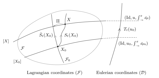
Figure 2. A schematic illustration of the construction of the semigroup. The set $\mathcal{F}$ where the Lagrangian variables are defined is represented by the interior of the closed domain on the left. The equivalence classes $[X]$ and $[X_{0}]$ (with respect to the action of the relabeling group $G$) of $X$ and $X_{0}$, respectively, are represented by the horizontal curves. To each equivalence class there corresponds a unique element in $\mathcal{F}_{0}$ and $\mathcal{D}$ (the set of Eulerian variables). The sets $\mathcal{F}_{0}$ and $\mathcal{D}$ are represented by the vertical curves.

Definition 4.1.

The set $\mathcal{D}$ consists of all pairs $(u,\mu)$ such that

1. $u\in H^{1}(\mathbb{R})$, and

2. $\mu$ is a positive Radon measure whose absolutely continuous part $\mu_{ac}$ satisfies

   (4.1) $$\mu_{ac}=u^{2}+u_{x}^{2}.$$

We can define a mapping, denoted by $L$, from $\mathcal{D}$ to $\mathcal{F}_{0}$:

Definition 4.2.

For any $(u,\mu)$ in $\mathcal{D}$ let,

(4.2) $$\left\{\begin{aligned} y(\xi)&=\sup\{y\mid\mu((-\infty,y))+y<\xi\},\\ H(\xi)&=\xi-y(\xi),\\ U(\xi)&=u\circ y(\xi).\end{aligned}\right.$$

Then $(y,U,H)\in\mathcal{F}_{0}$, and we denote by $L:\mathcal{D}\to\mathcal{F}_{0}$ the map which to any $(u,\mu)$ associates $X\in\mathcal{F}_{0}$.

Thus from any initial data $(u_{0},\mu_{0})\in\mathcal{D}$, we can construct a solution of (2.11) in $\mathcal{F}$ with initial data $X_{0}=L(u_{0},\mu_{0})\in\mathcal{F}_{0}$. It remains to go back to the original variables, which is the purpose of the mapping $M$ defined as follows:

Definition 4.3.

Given any element $X$ in $\mathcal{F}_{0}$, then $(u,\mu)$ defined as follows

(4.3) $$u(x)=U(\xi)\text{ for any }\xi\text{ such that }x=y(\xi),$$

(4.4) $$\mu=y_{\#}(\nu d\xi),$$

belongs to $\mathcal{D}$. We denote by $M:\mathcal{F}_{0}\to\mathcal{D}$ the map which to any $X$ in $\mathcal{F}_{0}$ associates $(u,\mu)$.

In fact, $M$ can be seen as a map from $\mathcal{F}/G\to D$, as any two elements belonging to the same equivalence class in $\mathcal{F}$ are mapped to the same element in $\mathcal{D}$ (cf. [13]). Moreover, identifying elements belonging to the same equivalence class, the mappings $L$ and $M$ are invertible and

(4.5) $$L\circ M=\operatorname{Id}_{\mathcal{F}/G},\quad\text{ and }\quad M\circ L=\operatorname{Id}_{\mathcal{D}}.$$

We will now use these mappings for defining also a Lipschitz metric on $\mathcal{D}$.

Definition 4.4.

Let

(4.6) $$T_{t}:=MS_{t}L\colon\mathcal{D}\rightarrow\mathcal{D}.$$

Next we show that $T_{t}$ is a Lipschitz continuous semigroup by introducing a metric on $\mathcal{D}$. Using the map $L$ we can transport the topology from $\mathcal{F}_{0}$ to $\mathcal{D}$.

Definition 4.5.

Define the metric $d_{\mathcal{D}}\colon\mathcal{D}\times\mathcal{D}\rightarrow[0,\infty)$ by

(4.7) $$d_{\mathcal{D}}((u,\mu),(\tilde{u},\tilde{\mu}))=d(L(u,\mu),L(\tilde{u},\tilde{\mu})).$$

The Lipschitz stability of the semigroup $T_{t}$ follows then naturally from Theorem 3.10. It holds on sets of bounded energy, which are given as follows.

Definition 4.6.

Given $M>0$, we define the subsets $\mathcal{D}^{M}$ of $\mathcal{D}$, which correspond to sets of bounded energy, as

(4.8) $$\mathcal{D}^{M}=\{(u,\mu)\in\mathcal{D}\ |\ \mu(\mathbb{R})\leq M\}.$$

On the set $\mathcal{D}^{M}$ we define the metric $d_{\mathcal{D}^{M}}$ as

(4.9) $$d_{\mathcal{D}^{M}}((u,\mu),(\tilde{u},\tilde{\mu}))=d^{M}(L(u,\mu),L(\tilde{u},\tilde{\mu})),$$

where the metric $d^{M}$ is defined as in Definition 3.9.

Definition 4.6 is well-posed as we can check from the definition of $L$: If $(u,\mu)\in\mathcal{D}^{M}$, then $L(u,\mu)\in\mathcal{F}_{0}^{M}$.

Theorem 4.7.

The semigroup $(T_{t},d_{\mathcal{D}})$ is a continuous semigroup on $\mathcal{D}$ with respect to the metric $d_{D}$. The semigroup is Lipschitz continuous on sets of bounded energy, that is: Given $M>0$ and a time interval $[0,T]$, there exists a constant $C_{M}$, which only depends on $M$ and $T$ such that for any $(u,\mu)$ and $(\tilde{u},\tilde{\mu})$ in $\mathcal{D}^{M}$, we have

(4.10) $$d_{D^{M}}(T_{t}(u,\mu),T_{t}(\tilde{u},\tilde{\mu}))\leq C_{M}d_{\mathcal{D}^{M}}((u,\mu),(\tilde{u},\tilde{\mu}))$$

for all $t\in[0,T]$.

Proof.

First we prove that $T_{t}$ is a semigroup. Since $\bar{S}_{t}$ is a mapping from $\mathcal{F}_{0}$ to $\mathcal{F}_{0}$, we have

$$T_{t}T_{t^{\prime}}=M\bar{S}_{t}LM\bar{S}_{t^{\prime}}L=M\bar{S}_{t}\bar{S}_{t^{\prime}}L=M\bar{S}_{t+t^{\prime}}L=T_{t+t^{\prime}}$$

where we also used (4.5) and the semigroup property of $\bar{S}_{t}$. We now prove the Lipschitz continuity of $T_{t}$. By using Theorem 3.10, we obtain that

$$d_{\mathcal{D}^{M}}(T_{t}(u,\mu),T_{t}(\tilde{u},\tilde{\mu})) =d^{M}(LM\bar{S}_{t}L(u,\mu)LM\bar{S}_{t}L(\tilde{u},\tilde{\mu}))$$

$$=d^{M}(\bar{S}_{t}L(u,\mu),\bar{S}_{t}L(\tilde{u},\tilde{\mu}))$$

(4.11) $$\leq C_{M}d^{M}(L(u,\mu),L(\tilde{u},\tilde{\mu}))$$

$$=C_{M}d_{\mathcal{D}^{M}}((u,\mu),(\tilde{u},\tilde{\mu})).$$

∎

By a weak solution of the Camassa–Holm equation we mean the following.

Definition 4.8.

Let $u\colon\mathbb{R}\times\mathbb{R}\rightarrow\mathbb{R}$ that satisfies

1. $u\in L^{\infty}([0,\infty),H^{1}(\mathbb{R}))$,

2. the equations

   (4.12) $$\iint_{\mathbb{R}_{+}\times\mathbb{R}}-u(t,x)\phi_{t}(t,x)+(u(t,x)u_{x}(t,x)+P_{x}(t,x))\phi(t,x)dxdt=\int_{\mathbb{R}}u(0,x)\phi(0,x)dx,$$

   and

   (4.13) $$\iint_{\mathbb{R}_{+}\times\mathbb{R}}(P(t,x)-u^{2}(t,x)-\frac{1}{2}u_{x}^{2}(t,x))\phi(t,x)+P_{x}(t,x)\phi_{x}(t,x)dxdt=0,$$

hold for all $\phi\in C_{0}^{\infty}([0,\infty),\mathbb{R})$. Then we say that $u$ is a weak global solution of the Camassa–Holm equation.

Theorem 4.9.

Given any initial condition $(u_{0},\mu_{0})\in\mathcal{D}$, we denote $(u,\mu)(t)=T_{t}(u_{0},\mu_{0})$. Then $u(t,x)$ is a weak, global solution of the Camassa–Holm equation.

Proof.

After making the change of variables $x=y(t,\xi)$ we get on the one hand

$$-\iint_{\mathbb{R}_{+}\times\mathbb{R}} u(t,x)\phi_{t}(t,x)dxdt=-\iint_{\mathbb{R}_{+}\times\mathbb{R}}u(t,y(t,\xi))\phi_{t}(t,y(t,\xi))y_{\xi}(t,\xi)d\xi dt$$

$$=-\iint_{\mathbb{R}_{+}\times\mathbb{R}}U(t,\xi)[(\phi(t,y(t,\xi))_{t}-\phi_{x}(t,y(t,\xi)))y_{t}(y,\xi)]y_{\xi}(t,\xi)d\xi dt$$

$$=-\iint_{\mathbb{R}_{+}\times\mathbb{R}}[U(t,\xi)y_{\xi}(t,\xi)(\phi(t,y(t,\xi)))_{t}-\phi_{\xi}(t,y(t,\xi))U(t,\xi)^{2}]d\xi dt$$

(4.14) $$=\int_{\mathbb{R}}U(0,\xi)\phi(0,y(0,\xi))y_{\xi}(0,\xi)d\xi$$

$$\quad+\iint_{\mathbb{R}_{+}\times\mathbb{R}}[U_{t}(t,\xi)y_{\xi}(t,\xi)+U(t,\xi)y_{\xi t}(t,\xi)]\phi(t,y(t,\xi))d\xi dt$$

$$\quad+\iint_{\mathbb{R}_{+}\times\mathbb{R}}U^{2}(t,\xi)\phi_{\xi}(t,y(t,\xi))d\xi dt$$

$$=\int_{\mathbb{R}}u(0,x)\phi(0,x)dx$$

$$\quad-\iint_{\mathbb{R}_{+}\times\mathbb{R}}(Q(t,\xi)y_{\xi}(t,\xi)+U_{\xi}(t,\xi)U(t,\xi))\phi(t,y(t,\xi))d\xi dt,$$

while on the other hand

$$\iint_{\mathbb{R}_{+}\times\mathbb{R}} (u(t,x)u_{x}(t,x)+P_{x}(t,x))\phi(t,x)dxdt$$

(4.15) $$=\iint_{\mathbb{R}_{+}\times\mathbb{R}}(U(t,\xi)U_{\xi}(t,\xi)+P_{x}(t,y(t,\xi))y_{\xi}(t,\xi))\phi(t,y(t,\xi))d\xi dt$$

$$=\iint_{\mathbb{R}_{+}\times\mathbb{R}}(U(t,\xi)U_{\xi}(t,\xi)+Q(t,\xi)y_{\xi}(t,\xi))\phi(t,y(t,\xi))d\xi dt,$$

which shows that (4.12) is fulfilled. Equation (4.13) can be shown analogously

$$\iint_{\mathbb{R}_{+}\times\mathbb{R}} P_{x}(t,x)\phi_{x}(t,x)dxdt$$

$$=\iint_{\mathbb{R}_{+}\times\mathbb{R}}Q(t,\xi)y_{\xi}(t,\xi)\phi_{x}(t,y(t,\xi))d\xi dt$$

(4.16) $$=\iint_{\mathbb{R}_{+}\times\mathbb{R}}Q(t,\xi)\phi_{\xi}(t,y(t,\xi))d\xi dt$$

$$=-\iint_{\mathbb{R}_{+}\times\mathbb{R}}Q_{\xi}(t,\xi)\phi(t,y(t,\xi))d\xi dt$$

$$=\iint_{\mathbb{R}_{+}\times\mathbb{R}}[\frac{1}{2}H_{\xi}(t,\xi)+(\frac{1}{2}U^{2}(t,\xi)-P(t,\xi))y_{\xi}(t,\xi)]\phi(t,y(t,\xi))d\xi dt$$

$$=\iint_{\mathbb{R}_{+}\times\mathbb{R}}[\frac{1}{2}u_{x}^{2}(t,x)+u^{2}(t,x)-P(t,x)]\phi(t,x)dxdt.$$

In the last step we used the following

(4.17) $$\int_{\mathbb{R}}u^{2}+u_{x}^{2}dx =\int_{\mathbb{R}}u^{2}\circ yy_{\xi}+u^{2}_{\xi}\circ yy_{\xi}d\xi$$

$$=\int_{\{\xi\in\mathbb{R}\mid y_{\xi}(t,\xi)>0\}}U^{2}y_{\xi}+\frac{U_{\xi}^{2}}{y_{\xi}}d\xi=\int_{\mathbb{R}}H_{\xi}d\xi.$$

For almost every $t\in\mathbb{R}_{+}$ the set $\{\xi\in\mathbb{R}\mid y_{\xi}(t,\xi)>0\}$ is of full measure and hence

(4.18) $$\int_{\mathbb{R}}u^{2}+u_{x}^{2}dx=\int_{\mathbb{R}}H_{\xi}d\xi,$$

which is bounded by a constant for all times. Thus we proved that $u$ is a weak solution of the Camassa–Holm equation. ∎

5. The topology on $\mathcal{D}$

Proposition 5.1.

The mapping

(5.1) $$u\mapsto(u,(u^{2}+u_{x}^{2})dx)$$

is continuous from $H^{1}(\mathbb{R})$ into $\mathcal{D}$. In other words, given a sequence $u_{n}\in H^{1}(\mathbb{R})$ converging to $u\in H^{1}(\mathbb{R})$, then $(u_{n},(u_{n}^{2}+u_{nx}^{2})dx)$ converges to $(u,(u^{2}+u_{x}^{2})dx)$ in $\mathcal{D}$.

Proof.

Let $X_{n}=(y_{n},U_{n},H_{n})=L(u_{n},(u_{n}^{2}+u_{nx}^{2})dx)$ and $X=(y,U,H)=L(u,(u^{2}+u_{x}^{2})dx)$. Then as in the proof of [13, Proposition 5.1] one can show that

(5.2) $$X_{n}\to X\text{ in }E.$$

Hence using (3.9), we get that $\lim_{n\to\infty}d(X_{n},X)=0$. ∎

Proposition 5.2.

Let $(u_{n},\mu_{n})$ be a sequence in $\mathcal{D}$ that converges to $(u,\mu)$ in $\mathcal{D}$. Then

(5.3) $$u_{n}\rightarrow u\text{ in }L^{\infty}(\mathbb{R})\text{ and }\mu_{n}\overset{\ast}{\rightharpoonup}\mu.$$

Proof.

Let $X_{n}=(y_{n},U_{n},H_{n})=L(u_{n},\mu_{n})$ and $X=(y,U,H)=L(u,\mu)$ . By the definition of the metric $d_{\mathcal{D}}$, we have $\lim_{n\to\infty}d(X_{n},X)=0$. Using (3.9), we immediately obtain that

(5.4) $$X_{n}\to X\text{ in }L^{\infty}(\mathbb{R}).$$

The rest can be proved as in [13, Proposition 5.2]. ∎

Acknowledgments. K. G. gratefully acknowledges the hospitality of the Department of Mathematical Sciences at the NTNU, Norway, creating a great working environment for research during the fall of 2009.

References

- [1] A. Bressan and A. Constantin. Global conservative solutions of the Camassa–Holm equation. Arch. Ration. Mech. Anal. 183:215–239, 2007.
- [2] A. Bressan, H. Holden, and X. Raynaud. Lipschitz metric for the Hunter–Saxton equation. J. Math. Pures Appl. 94:68–92, 2010.
- [3] R. Camassa and D. D. Holm. An integrable shallow water equation with peaked solutions. Phys. Rev. Lett 71(11):1661–1664, 1993.
- [4] R. Camassa, D. D. Holm, and J. Hyman. A new integrable shallow water equation. Adv. Appl. Mech 31:1–33, 1994.
- [5] A. Constantin and J. Escher. Global existence and blow-up for a shallow water equation. Ann. Scuola Norm. Sup. Pisa Cl. Sci. (4) 26:303–328, 1998.
- [6] A. Constantin and J. Escher. Wave breaking for nonlinear nonlocal shallow water equations. Acta Math. 181:229–243, 1998.
- [7] A. Constantin and J. Escher. On the blow-up rate and the blow-up set of breaking waves for a shallow water equation. Math. Z. 233:75–91, 2000.
- [8] A. Constantin and D. Lannes. The hydrodynamical relevance of the Camassa–Holm and Degasperis–Procesi equations. Arch. Rat. Mech. Anal., 192:165–186, 2009.
- [9] H.-H. Dai. Exact traveling-wave solutions of an integrable equation arising in hyperelastic rods. Wave Motion, 28(4):367–381, 1998.
- [10] H.-H. Dai. Model equations for nonlinear dispersive waves in a compressible Mooney–Rivlin rod. Acta Mech., 127(1-4):193–207, 1998.
- [11] H.-H. Dai and Y. Huo. Solitary shock waves and other travelling waves in a general compressible hyperelastic rod. Proc. R. Soc. Lond. Ser. A Math. Phys. Eng. Sci., 456(1994):331–363, 2000.
- [12] K. Grunert, H. Holden, and X. Raynaud. Lipschitz metric for the periodic Camassa–Holm equation. J. Differential Equations doi:10.1016/j.jde.2010.07.006, 2010.
- [13] H. Holden and X. Raynaud. Global conservative solutions of the Camassa–Holm equation—a Lagrangian point of view. Comm. Partial Differential Equations 32:1511–1549, 2007.
- [14] H. Holden and X. Raynaud. Global conservative multipeakon solutions of the Camassa–Holm equation. J. Hyperbolic Differ. Equ. 4:39–64, 2007.
- [15] H. Holden and X. Raynaud. Global conservative solutions of the generalized hyperelastic-rod wave equation. J. Differential Equations 233:448–484, 2007.