Approximation of conditional densities by smooth mixtures of regressions

Abstract

This paper shows that large nonparametric classes of conditional multivariate densities can be approximated in the Kullback–Leibler distance by different specifications of finite mixtures of normal regressions in which normal means and variances and mixing probabilities can depend on variables in the conditioning set (covariates). These models are a special case of models known as “mixtures of experts” in statistics and computer science literature. Flexible specifications include models in which only mixing probabilities, modeled by multinomial logit, depend on the covariates and, in the univariate case, models in which only means of the mixed normals depend flexibly on the covariates. Modeling the variance of the mixed normals by flexible functions of the covariates can weaken restrictions on the class of the approximable densities. Obtained results can be generalized to mixtures of general location scale densities. Rates of convergence and easy to interpret bounds are also obtained for different model specifications. These approximation results can be useful for proving consistency of Bayesian and maximum likelihood density estimators based on these models. The results also have interesting implications for applied researchers.

1 Introduction

This paper explores approximation properties of finite smooth mixtures of normal regressions as flexible models for conditional densities. These models are a special case of mixtures of experts (ME) introduced by Jacobs et al. (1991). ME have become increasingly popular is statistical literature since they are very flexible, easy to interpret and reasonably easy to estimate. See, for example, papers by Jordan and Jacobs (1994) and Jordan and Xu (1995) who employ the expectation maximization (EM) estimation algorithm or papers by Peng, Jacobs and Tanner (1996), Wood, Jiang and Tanner (2002), Geweke and Keane (2007) andVillani, Kohn and Giordani (2009) who use Markov chain Monte Carlo methods for estimation of ME in the Bayesian framework. This paper contributes to the literature that provides a theoretical explanation of the success of ME models in applications. In particular, I show that large classes of conditional densities can be approximated in the Kullback–Leibler (KL) distance by finite smooth mixtures of normal regressions. Approximation results are obtained in the KL distance for the following reason. If a data generating density is in the KL closure of a class of models then this density can be consistently estimated from data by these models under weak regularity conditions [see, e.g., Ghosh and Ramamoorthi (2003) for a textbook treatment of Schwarz’s theorem on posterior consistency and Roeder and Wasserman (1997) for posterior consistency results for finite mixture of normals].

Consider a joint probability distribution $F$ on a product space $Y\times X$, $Y\subset R^{d}$ and $X\subset R^{d_{x}}$. Assume the conditional distribution $F(y|x)$ has a density $f(y|x)$ with respect to the Lebesgue measure. The marginal density of $x$ with respect to some generic measure is denoted by $f(x)$. A model $\mathcal{M}$ for the conditional density $f(y|x)$ is described by $p(y|x,\mathcal{M})$. The KL distance between $f(y|x)f(x)$ and $p(y|x,\mathcal{M})f(x)$ is defined by

$$d_{\mathrm{KL}}(F,\mathcal{M})=\int\log\frac{f(y|x)}{p(y|x,\mathcal{M})}F(dy,dx).$$

This distance can also be interpreted as the expected KL distance between the conditional distributions. Either way, this is the distance useful for obtaining estimation consistency results. Also, convergence in the KL distance implies convergence in the total variation distance. Below, I consider several different specifications of mixture of normal regressions models, $p(y|x,\mathcal{M})$, and provide conditions on $F$ under which $d_{\mathrm{KL}}(F,\mathcal{M})$ can be made arbitrarily small. I also derive rates of convergence and easy to interpret bounds for $d_{\mathrm{KL}}(F,\mathcal{M})$.

In general, a finite mixture of normal regressions model can be written as

$$p(y|x,\mathcal{M})=\sum_{j=1}^{m}\alpha_{j}^{m}(x)\phi(y,\mu_{j}^{m}(x),\sigma_{j}^{m}(x)),$$

where mixing probabilities satisfy $\alpha_{j}^{m}(x)\in[0,1]$ and $\sum_{j}\alpha_{j}^{m}(x)=1$, and $\phi(y,\mu$, $\sigma)$ is a normal density with mean $\mu$ and standard deviation $\sigma$ evaluated at $y$ (if $y$ is multidimensional then the variance–covariance matrix is diagonal $\sigma^{2}I$). Most of the results obtained in the paper can be easily extended to models in which general location scale densities $\sigma^{-d}K((y-\mu)/\sigma)$ are mixed instead of the normal densities $\phi(y,\mu,\sigma)$. Models, in which the mixing weights depend on $x$, are referred in this paper as smooth mixtures. In practice, $\alpha_{j}^{m}(x)$’s are often modeled by a multinomial choice model, for example, multinomial logit [Peng, Jacobs and Tanner (1996)] or probit [Geweke and Keane (2007)], or it might not depend on $x$. The mean $\mu_{j}^{m}(x)$ can be constant, linear or flexible, for example, polynomial, in $x$. An exponentiated polynomial or spline in $x$ can be used for modeling the standard deviation $\sigma_{j}^{m}(x)$ [Villani, Kohn and Giordani (2009)].

To the best of my knowledge, previous literature on smooth mixtures of regressions (or experts) does not provide a theory on what specifications for $\alpha_{j}^{m}$, $\mu_{j}^{m}$ and $\sigma_{j}^{m}$ deliver a model that can approximate and consistently estimate large nonparametric classes of densities $F$. There are theoretical results on approximation of smooth functions and estimation of conditional expectations by ME [see Zeevi, Meir and Maiorov (1998) and Maiorov and Meir (1998)]. The only paper on approximation of conditional densities by ME seems to be Jiang and Tanner (1999) who develop approximation and estimation results for target densities from a single parameter exponential family, in which the parameter is a smooth function of covariates. A detailed comparison with results in Jiang and Tanner (1999) is presented in Section 6. In this paper, I do not restrict the functional form of $f(y|x)$ and use weak regularity conditions to describe a class of $F$ that can be approximated. Conditions on approximable classes of $f(y|x)$ and $f(x)$ that are common for different model specifications include bounded support for $f(x)$, continuity of $f(y|x)$ in $(y,x)$, finite expectation of a change of $\log f(y|x)$ in a neighborhood of $y$ and existence of the second moments of $y$. The latter restriction can be weakened by adding densities with fat tails to the mixtures in addition to normal densities.

In Section 4, I show that considerable flexibility is already attained when $\alpha_{j}^{m}$’s are modeled by multinomial logit with linear indices in $x$, and $(\mu_{j}^{m},\sigma_{j}^{m})$ are independent of $x$. Results in Sections 3 and 4 suggest that using polynomials in the logit specification reduces the number of mixture components $m$ required to achieve a specified approximation precision. As shown in Section 5, models for univariate response $y$ in which the mixing probabilities and the variances of the mixed normals are independent of $x$, and the means are flexible, for example, polynomial in $x$, can approximate large classes of $f(y|x)$. Differences in quantiles of $f(y|x)$ from these classes have to be bounded above and below uniformly in $x$. These restrictions on $f(y|x)$ can be weakened if the variances of the mixed normals are modeled by flexible functions of $x$. Section 7 summarizes the findings.

2 Infeasible model

In this section, I explicitly construct a smooth mixture of normals model that converges to a given $F$ in the KL distance as $m$ increases. This model is not feasible in the sense that it is not based on components employed in practice, for example, logit/probit mixing probabilities. However, the results for feasible models presented in the following sections follow from this one or are similar.

Let $A_{j}^{m}$, $j=0,1,\ldots,m$, be a partition of $Y$ consisting of adjacent half-open half-closed hypercubes $A_{1}^{m},\ldots,A_{m}^{m}$ with side length $h_{m}$ and the rest of the space $A_{0}^{m}$. As $m$ increases the fine part of the partition becomes finer, $h_{m}\rightarrow 0$. Also, it covers larger and larger part of $Y$: for any $y\in Y$ there exists $M_{0}$ such that

$$\forall m\geq M_{0}\qquad C_{\delta_{m}}(y)\cap A_{0}^{m}=\varnothing,$$ (1)

where $C_{\delta_{m}}(y)$ is a hypercube with center $y$ and side length $\delta_{m}\rightarrow 0$. It is always possible to construct such a partition. For example, if $Y=[0,\infty)$ let $A_{0}^{m}=[\log m,\infty)$, $A_{j}^{m}=[(j-1)\log m/m,j\log m/m)$ for $j\neq 0$, and $h_{m}=\log m/m$.

A candidate model $\mathcal{M}_{0}$ for approximating $f(y|x)$ is

$$p(y|x,\mathcal{M}_{0})=\sum_{j=1}^{m}F(A_{j}^{m}|x)\phi(y,\mu_{j}^{m},\sigma_{m})+F(A_{0}^{m}|x)\phi(y,0,\sigma_{0}),$$ (2)

where $\sigma_{0}$ is fixed, $\sigma_{m}$ converges to zero as $m$ increases and $\mu_{j}^{m}$ is the center of $A_{j}^{m}$. One can always construct a model $\mathcal{M}_{0}$ and a partition $A_{j}^{m}$ so that

$$\delta_{m}\rightarrow 0,\qquad\sigma_{m}/\delta_{m}\rightarrow 0,\qquad\delta_{m}^{d-1}h_{m}/\sigma_{m}^{d}\rightarrow 0,$$ (3)

for example, in the example for $Y=[0,\infty)$ from the previous paragraph let $\sigma_{m}=h_{m}^{0.5}$ and $\delta_{m}=h_{m}^{0.25}$.

For a partition satisfying (1) and (3), let us introduce the following restrictions on $F$.

Assumption 2.1.

1. f(y|x) is continuous in $y$ a.s. $F$.

1. [2.]

2. The second moments of $y$ are finite.

3. For any $(y,x)$ there exists a hypercube $C(r,y,x)$ with side length $r>0$ and $y\in C(r,y,x)$ such that (i)

   $$\int\log\frac{f(y|x)}{\inf_{z\in C(r,y,x)}f(z|x)}F(dy,dx)<\infty$$ (4)

   and (ii) exists $M_{3}$ such that for any $m\geq M_{3}$, if $y\in A_{0}^{m}$ then $C(r,y,x)\cap A_{0}^{m}$ contains a hypercube $C_{0}(r,y,x)$ with side length $r/2$ and a vertex at $y$ and if $y\in Y\setminus A_{0}^{m}$, then $C(r,y,x)\cap(Y\setminus A_{0}^{m})$ contains a hypercube $C_{1}(r,y,x)$ with side length $r/2$ and a vertex at $y$.

Parameter $\sigma_{0}$ can always be chosen so that

$$1>2^{-(d+1)}>\phi(y,0,\sigma_{0})\lambda(C_{0}(r,y,x)),$$ (5)

where $\lambda$ is the Lebesgue measure.

Proposition 2.1.

If the model $p(y|x,\mathcal{M}_{0})$ and the partition $A_{j}^{m}$ are constructed so that (1), (2), (3) and (5) hold, and $F$ satisfies Assumption 2.1, then $d_{\mathrm{KL}}(F,\mathcal{M}_{0})\rightarrow 0$ as $m\rightarrow\infty$.

The proposition is rigorously proved in the Appendix. Here, I briefly describe the intuition behind the argument and the role of the assumptions. Convergence in the KL distance is proved by the dominated convergence theorem (DCT). First, I establish point-wise convergence of the integrand, $\log f(y|x)/p(y|x,\mathcal{M}_{0})$, to zero, and then I derive an integrable upper bound on the integrand for the DCT applicability. Nonnegativity of the KL distance is fruitfully exploited in the proof as it allows working only with upper bounds and ignoring the lower ones in convergence arguments.

The first term on the right-hand side of (2) (the sum from 1 to $m$) approximates the integral

$$\int\phi(y,\mu,\sigma_{m})f(\mu|x)\,d\mu=\int f(y-\sigma_{m}z|x)\phi(z,0,1)\,dz,$$ (6)

when $h_{m}$ is much smaller than $\sigma_{m}$, and the fine part of the partition is large. The integral on the right-hand side of (6) is obtained by the change of variables. For a small $\delta_{m}$ and $z$ satisfying $\|\sigma_{m}z\|\leq\delta_{m}$, $f(y-\sigma_{m}z|x)$ is close to $f(y|x)$ as $f(y|x)$ is assumed to be continuous in $y$. Therefore, when $\sigma_{m}$ is much smaller than $\delta_{m}$ the right-hand side of (6) should be close to $f(y|x)$. Thus, this intuitive argument explains the role of conditions (3) and continuity of $f(y|x)$.

The second term on the right-hand side of (2) converges to zero. This term is not needed for point-wise convergence. It can be omitted when the support of $f(y|x)$ is bounded uniformly in $x$ as in this case we can set $A_{0}^{m}=\varnothing$ and use the same variance $\sigma_{m}^{2}$ in all mixture components (there is no need to define $\sigma_{0}$). This term together with part 2 of Assumption 2.1 prevents tails of $p(y|x,\mathcal{M}_{0})$ from becoming too thin relative to $f(y|x)$ in the unbounded support case (in the absence of this term the tails would be too thin as $\sigma_{m}\rightarrow 0$).

Parts 2 and 3 of Assumption 2.1 together guarantee existence of an integrable upper bound for the DCT applicability. An upper bound on $\log f(y|x)/p(y|x$, $\mathcal{M}_{0})$ involves a lower bound on $p(y|x,\mathcal{M}_{0})$. Both terms on the right-hand side in the definition of $p(y|x,\mathcal{M}_{0})$ in (2) can be bounded below by an expression proportional to $\inf_{z\in C(r,y,x)}f(z|x)$. That is how condition (4) is deduced. The lower bound for the second term in (2) also includes $\phi(y,0,\sigma_{0})$ and that is why finiteness of the second moments of $y$ is assumed.

One interpretation of condition (4) [part 3(i) of Assumption 2.1] is that local relative changes in $f(y|x)$ due to changes in $y$ should not be infinitely large on average. It seems difficult to think of an unconditional density, which is well behaved and positive everywhere, that would violate (4). This part of the assumption though can be violated by reasonable conditional densities as Example 2.1 below illustrates.

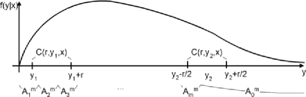
Figure 1: Construction of $C(r,y,x)$.

When $f(y|x)$ is positive everywhere, part 3(ii) of Assumption 2.1 is not needed. It always holds if $C(r,y,x)$ is a hypercube with center at $y$. Part 3(ii) becomes important when $f(y|x)$ can be equal to zero. In particular, the sets $C_{0}(r,y,x)$ and $C_{1}(r,y,x)$ in part 3(ii) of Assumption 2.1 are introduced to specify that $C(r,y,x)$ needs to be defined differently near the boundary of the support and in the tails if one wants to use condition (4) in its present form. This is illustrated in Figure 1.

The support of $f(\cdot|x)$ should include $C(r,y,x)$ a.s. $F$; otherwise, part 3(i) of Assumption 2.1 is not satisfied. Therefore, for $f(y|x)$ in Figure 1, it has to be the case that $C(r,y,x)=[y,y+r]$ at the boundary of the support (the intersection of the axes). Setting $C(r,y,x)=[y,y+r]$ near the boundary of the support makes the ratio $f(y|x)/\inf_{z\in C(r,y,x)}f(z|x)$ smallest possible (equal to one) and thus helps with condition (4). Parts of $Y$ near the boundary of the support are covered by the fine part of the partition $A_{1}^{m},\ldots,A_{m}^{m}$ for all sufficiently large $m$, and part 3(ii) of Assumption 2.1 holds for $C_{1}(r,y,x)=[y,y+r/2]$. Using $C(r,y,x)=[y,y+r]$ for all $y$ would not work. Since for any $m$ one can find $y\in A_{m}^{m}$ such that $C(r,y,x)\cap Y\setminus A_{0}^{m}$ is arbitrary small, and part 3(ii) of Assumption 2.1 fails. Thus, for $y$ that are arbitrary far from the boundary of the support, one has to use $C(r,y,x)=[y-r/2,y+r/2]$ eventually. Then, part 3(ii) of the assumption clearly holds for $C_{1}(r,y,x)=[y-r/2,y]$, $C_{0}(r,y,x)=[y,y+r/2]$ and any $m$.

Results in this section and similar results in the following sections can be generalized in several different ways. First, the derivation of the integrable upper bound in the proof of Proposition 2.1 suggests that the requirement of finite second moments of $y$ can be weakened by adding a density with thicker than normal tails to the mixture of normals; for example, substitute $\phi(y,0,\sigma_{0})$ in (2) with a Student $t$-density. Second, more general shapes of the support of $F$ can be accommodated if instead of hypercubes $C(r,y,x)$, $C_{0}(r,y,x)$, and $C_{1}(r,y,x)$ in Assumption 2.1 different sets with positive Lebesgue measure are used. For example, if the support of $f(\cdot|x)$ is a triangle in $R^{2}$ then small triangles can be used instead of the squares $C(r,y,x)$, $C_{0}(r,y,x)$ and $C_{1}(r,y,x)$. Third, general location scale densities $\sigma^{-d}K((y-\mu)/\sigma)$ can be used in mixtures instead of normal densities. As long as analogs of Lemmas .1, .2 and .3 (see the Appendix) are available for a particular type of densities, results in this and the following sections will hold for mixtures of these densities. Lemmas .1 and .3 hold for $\sigma^{-d}K((y-\mu)/\sigma)$ if $K(z)$ is bounded and nonincreasing in $|z|$ (proofs of the lemmas use only these facts about the normal distributions). The derivation of bounds in Lemma .2 exploits normality; however, the qualitative results of the lemma hold as long as $\int_{R}K(z)\,dz=1$ and $K(z)$ is positive in a neighborhood of zero. Thus, all the results in this paper that establish $d_{\mathrm{KL}}(F,\mathcal{M})\rightarrow 0$ do not depend on the normality assumption; however, bounds and convergence rates for $d_{\mathrm{KL}}(F,\mathcal{M})$ derived below are specific to mixtures of normal densities, and they might be different for mixtures of other densities. All these generalizations seem to be straight forward and I do not pursue them in this paper to keep the arguments short and simple.

Examples below demonstrate that Assumption 2.1 is satisfied for a large class of densities. They also describe some situations in which the assumption fails.

Example 2.1.

Exponential distribution, $f(y|x)=\gamma(x)\exp\{-\gamma(x)y\}$,$\gamma(x)>0$. The density is continuous in $y$ (part 1 of Assumption 2.1). Let $\int\gamma^{-2}\,dF<\infty$ so that the second moment of $y$ is finite (part 2 of Assumption 2.1). Define the partition $A_{j}^{m}$ and $C(r,y,x)$, $C_{0}(r,y,x)$ and $C_{1}(r,y,x)$ as shown in Figure 1, for example, for some $r>0$ let $C(r,y,x)=[y,y+r]$ for $y\in[0,r]$ and $C(r,y,x)=[y-r/2,y+r/2]$ for $y\in(r,\infty)$. Thus, from the discussion of Figure 1 above it follows that part 3(ii) of Assumption 2.1 is satisfied. Because $\log f(y|x)/\inf_{z\in C(r,y,x)}f(z|x)\leq r\gamma(x)$, part 3(i) of Assumption 2.1 holds as long as $\gamma(x)$ is integrable with respect to $f(x)$. If $\gamma(x)$ is not integrable, then part 3(i) of the assumption fails.

Example 2.2.

A Student $t$-distribution, in which scale and location parameters are functions of $x$, $f(y|x)\propto[\nu+((y-b(x))/c(x))^{2}]^{-(\nu+1)/2}$, $\nu>2$ and $b(x)^{2}$, $c(x)^{-2}$ and $c(x)^{2}$ are integrable w.r.t. $f(x)$. The second moment of $y$ is finite since

$$\int y^{2}\,dF = \int\biggl{(}c(x)^{2}\biggl{[}\frac{y-b(x)}{c(x)}\biggr{]}^{2}+2b(x)y-b(x)^{2}\biggr{)}\,dF$$

$$= \int\biggl{(}c(x)^{2}\frac{\nu}{\nu-2}+2b(x)^{2}-b(x)^{2}\biggr{)}\,dF<\infty.$$

As I discuss above, for densities positive everywhere part 3(ii) of Assumption 2.1 always holds with $C(r,y,x)=[y-r/2,y+r/2]$. Part 3(i) of Assumption 2.1 is also satisfied because

$$\int\log\frac{f(y|x)}{\inf_{z\in C(r,y,x)}f(z|x)}F(dy,dx)$$

$$\qquad=2\int_{X}\int_{b(x)}^{\infty}-\frac{\nu+1}{2}\log\frac{\nu+((y-b(x))/c(x))^{2}}{\nu+((y+r-b(x))/c(x))^{2}}f(y|x)\,dyF(dx)$$

$$\qquad\leq(\nu+1)2\int_{X}\int_{b(x)}^{\infty}\bigl{[}\nu+\bigl{(}\bigl{(}y+r-b(x)\bigr{)}/c(x)\bigr{)}^{2}\bigr{]}f(y|x)\,dyF(dx)<\infty,$$

where the last inequality follows by the integrability of $((y-b(x))/c(x)$, its square and $c(x)^{-2}$.

Example 2.3.

Suppose that conditional density $f(y|x)$ is continuous in $y$ and bounded above and away from zero, $\infty>\overline{f}\geq f(y|x)\geq\underline{f}>0$ for any $y\in Y=[a,b]$ and $x\in X$. Then we can set $A_{0}^{m}=\varnothing$. For $r\in(0,(b-a)/4)$, let $C(r,y,x)=[y,y+r]$ and $C_{1}(r,y,x)=[y,y+r/2]$ for $y\in[a,(a+b)/2]$ and $C(r,y,x)=[y-r,y]$ and $C_{1}(r,y,x)=[y-r/2,y]$ for $y\in((a+b)/2,b]$. Clearly, part 3(ii) of Assumption 2.1 is satisfied. Because $f(y|x)/\inf_{z\in C(r,y,x)}f(z|\break x)\leq\overline{f}/\underline{f}$ part 3(i) of Assumption 2.1 also holds. The second moment of $y$ is finite and thus all parts of Assumption 2.1 hold.

The boundedness away from zero condition can be replaced by a monotonicity condition at the boundary of the support. For example, let $f(y|x)$ be nondecreasing on $[a,a+2r]$, nonincreasing on $[b-2r,b]$ and bounded below by $\underline{f}>0$ on $[a+r,b-r]$. In this case $f(y|x)/\operatorname{inf}_{z\in C(r,y,x)}f(z|x)\leq\operatorname{max}\{1,\overline{f}/\underline{f}\}$ for any $y\in[a,b]$. Thus, part 3(i) of Assumption 2.1 holds. The other parts of the assumption are not affected by this change.

Example 2.4.

Consider a uniform distribution $f(y|x)=x^{-1}1_{[0,x]}(y)$ and $f(x)>0$ for any $x\in[1,\infty)$. A natural choice of the partition would be $A_{0}^{m}=[mh_{m},\infty)$ and $A_{j}^{m}=[(j-1)h_{m},jh_{m})$ for $j\in\{1,\ldots,m\}$. When $y=x$, the only reasonable choice of $C(r,y,x)$ is $C(r,y,x)=[y-r,y]$. For an arbitrary $m$ and $y=x=mh_{m}+r/4$, $C(r,y,x)$ violates part 3(ii) of Assumption 2.1 since the only possible $C_{0}(r,y,x)=[y-r/2,y]$ is not included in $A_{0}^{m}$. For $f(x)$ with bounded support, this example would satisfy Assumption 2.1 since in this case we could set $A_{0}^{m}=\varnothing$.

This example illustrates that Assumption 2.1 rules out some cases in which the support of $f(\cdot|x)$ is increasing in $x$ without a bound. In Section 5, I consider model specifications in which means and variances of the mixed normals can be flexible functions of $x$. Those specifications seem to be more promising for modeling densities $f(\cdot|x)$ with support increasing in $x$ without a bound (see Example 5.2).

2.1 Approximation error bounds

The proof techniques of this section can also be used to derive explicit bounds on the approximation error. The bounds for positive everywhere and especially differentiable $f(y|x)$ are particularly informative. It is also easy to deduce an approximation rate from them. Thus, I present below the bounds and approximation rate for these special albeit important cases. Convergence rates and bounds for other special classes can be obtained in a similar way, for example, for densities bounded away from zero. However, rates and bounds for the general case seem to be difficult to calculate.

Corollary 2.1.

Part (i). Suppose the model $p(y|x,\mathcal{M}_{0})$ and the partition $A_{j}^{m}$ are constructed so that (1), (2), (3) and (5) hold. Suppose $f(y|x)$ is positive and continuous in $y$ on $Y=R^{d}$ for all $x$, second moments of $y$ are finite and (4) holds with $C(r,y,x)=C_{r}(y)$ taken to be a hypercube with center at $y$ and radius $r$. Then, for all sufficiently large $m$,

$$d_{\mathrm{KL}}(F,\mathcal{M}_{0}) \leq \int\log\frac{f(y|x)}{\inf_{z\in C_{\delta_{m}}(y)}f(z|x)}F(dy,dx)$$ (10)

$${}+2\frac{3d^{3/2}\delta_{m}^{d-1}h_{m}}{(2\pi)^{d/2}\sigma_{m}^{d}}+2\exp\biggl{\{}-\frac{(\delta_{m}/\sigma_{m})^{2}}{8}\biggr{\}}$$

$${}+\int_{B_{\delta_{m}}(A_{0}^{m})}\log\frac{f(y|x)}{\inf_{z\in C_{r}(y)}f(z|x)}F(dy,dx)$$

$${}+\int_{B_{\delta_{m}}(A_{0}^{m})}\biggl{[}\frac{y^{\prime}y}{2\sigma_{0}^{2}}-\log\frac{(r/2)^{d}}{(2\pi\sigma_{0}^{2})^{d/2}}\biggr{]}F(dy,dx),$$

where $B_{\delta_{m}}(A_{0}^{m})=\{(y,x)\dvtx C_{\delta_{m}}(y)\cap A_{0}^{m}\neq\varnothing\}$and bounds in (10)–(10) converge to zero as $m\rightarrow\infty$.

Part (ii). If $f(y|x)$ is continuously differentiable in $y$ for all $x$ and instead of (4) the following condition holds:

$$\int\sup_{z\in C_{r}(y)}\biggl{\|}\frac{d\log f(z|x)}{dz}\biggr{\|}F(dy,dx)<\infty,$$ (11)

then for all sufficiently large $m$,

$$\qquad d_{\mathrm{KL}}(F,\mathcal{M}_{0}) \leq \delta_{m}\cdot\frac{d^{1/2}}{2}\int\sup_{z\in C_{\delta_{m}}(y)}\biggl{\|}\frac{d\log f(z|x)}{dz}\biggr{\|}F(dy,dx)$$ (15)

$${}+2\frac{3d^{3/2}\delta_{m}^{d-1}h_{m}}{(2\pi)^{d/2}\sigma_{m}^{d}}+2\exp\biggl{\{}-\frac{(\delta_{m}/\sigma_{m})^{2}}{8}\biggr{\}}$$

$${}+\frac{rd^{1/2}}{2}\int_{B_{\delta_{m}}(A_{0}^{m})}\sup_{z\in C_{r}(y)}\biggl{\|}\frac{d\log f(z|x)}{dz}\biggr{\|}F(dy,dx)$$

$${}+\int_{B_{\delta_{m}}(A_{0}^{m})}\biggl{[}\frac{y^{\prime}y}{2\sigma_{0}^{2}}-\log\frac{(r/2)^{d}}{(2\pi\sigma_{0}^{2})^{d/2}}\biggr{]}F(dy,dx),$$

and bounds in (15)–(15) converge to zero as $m\rightarrow\infty$.

Part (iii). If, in addition to assumptions from part (ii), for some $q>2$ and some $i_{1}\in\{1,\ldots,d\}$

$$\int|y_{i}|^{q}F(dy)<\infty,\qquad i\in\{1,\ldots,d\},$$ (16)

and

$$\int|y_{i_{1}}|^{q-2}\sup_{z\in C_{r}(y)}\biggl{\|}\frac{d\log f(z|x)}{dz}\biggr{\|}F(dy,dx)<\infty,$$ (17)

then the approximation error bound can be written as

$$d_{\mathrm{KL}}(F,\mathcal{M}_{0})\leq c\cdot\biggl{(}\frac{1}{m}\biggr{)}^{1/(d\cdot[2+1/(q-2)+\varepsilon])},$$ (18)

where $\varepsilon>0$ can be arbitrarily close to zero and $c$ does not depend on $m$.

The corollary is proved in the Appendix. The bounds in part (i) of the corollary follow from the proof of Proposition 2.1. The bounds in part (ii) are derived from the bounds in part (i), and they are especially easy to interpret. The larger the “average” derivative of $\log f(y|x)$ is the smaller $\delta_{m}$ has to be to achieve a prespecified level for the right-hand side of (15). Constant $h_{m}$ has to be much smaller than $\sigma_{m}$, and $\sigma_{m}$ has to be much smaller than $\delta_{m}$ [condition (3)] so that (15) becomes sufficiently small. Size of (15) and (15) depends on how fast and by how much tails of $f(y|x)f(x)$ dominate $d\log f(y|x)/dy$, $y^{2}$, and a constant.

The approximation rate in part (iii) is derived from the bounds in part (ii). Expressions in (15) and (15) can be immediately converted in expressions in terms of $m$. To convert (15) and (15) in expressions in terms of $m$ one seems to need slightly more than integrability of ${\sup_{z\in C_{r}(y)}}\|d\log f(z|x)/dz\|$ [condition (17)] and slightly more than finiteness of the second moments of $y$ [condition (16)]. Under these conditions, (15) and (15) are bounded by $(h_{m}m^{1/d})^{-(q-2)}$ times a constant (see the corollary proof). An upper bound on $(h_{m}m^{1/d})^{-(q-2)}$, (15) and (15) gives the rate in (18). This upper bound has to be strictly larger than (18) with $\varepsilon=0$ as I show in the corollary proof. For distributions with exponentially declining tails, (15) and (15) can be decreasing exponentially in $h_{m}m^{1/d}$. In this case, one can set $q=\infty$ in (18) (see Example 5.3 below).

The dimension of $y$ enters the approximation bounds exponentially. The dimension of $x$ does not affect the bound and the approximation rate for the “infeasible” model because this model is constructed with the use of $F(A_{j}^{m}|x)$’s, which are unknown functions of $x$. The following sections shed some light on the role of the dimension of $x$ in approximating $f(y|x)$ by feasible models.

3 Flexible multinomial choice models for mixing probabilities

This section gives conditions under which approximation results for “infeasible” model $\mathcal{M}_{0}$ also hold for a model with logit mixing probabilities that include polynomial terms in $x$. It also shows how to extend these results to multinomial probit and other models for mixing probabilities.

Assumption 3.1.

$X$ is compact and for partitions $A_{j}^{m}$, $j=0,1,\ldots,m$ satisfying (1), $F(A_{j}^{m}|x)$ is a continuous function of $x$ on $X$ and $F(A_{j}^{m}|x)>0$ [the support of $f(\cdot|x)$ does not depend on $x$].

Under this assumption (by the Stone–Weierstrass theorem) for any sequence of $\varepsilon_{m}\rightarrow 0$, $\varepsilon_{m}>0$ there exist finite order polynomials in $x$, $P_{j}^{m}(x)$ such that

$$|{\log F(A_{j}^{m}|x)-P_{j}^{m}(x)}|<\varepsilon_{m}\qquad\forall x\in X,j=1,\ldots,m.$$ (19)

Let $p(y|x,\mathcal{M}_{1})$ denote a model with $\sigma_{j}^{m}$ and $\mu_{j}^{m}$ independent of $x$ and logit mixing probabilities,

$$\alpha_{j}^{m}(x,\mathcal{M}_{1}) = \frac{\exp\{P_{j}^{m}(x)\}}{\sum_{k=1}^{m}\exp\{P_{k}^{m}(x)\}}$$

$$= \frac{F(A_{j}^{m}|x)\exp\{P_{j}^{m}(x)-\log F(A_{j}^{m}|x)\}}{\sum_{k=1}^{m}F(A_{k}^{m}|x)\exp\{P_{k}^{m}(x)-\log F(A_{k}^{m}|x)\}}.$$

Condition (19) implies $\alpha_{j}^{m}(x,\mathcal{M}_{1})\in(F(A_{j}^{m}|x)\exp\{-2\varepsilon_{m}\},F(A_{j}^{m}|x)\exp\{2\varepsilon_{m}\})$. The following corollary immediately follows.

Corollary 3.1.

If Assumption 3.1 and the conditions of Proposition 2.1 hold then $d_{\mathrm{KL}}(F,\mathcal{M}_{1})$ is bounded above and below by $d_{\mathrm{KL}}(F,\mathcal{M}_{0})\pm 2\varepsilon_{m}$ and thus converges to zero.

It seems possible to extend this corollary to other models for mixing probabilities, in particular, to a class of multinomial choice models in which mixing probabilities have the following representation:

$$\alpha_{j}^{m}(x)=\operatorname{Pr}[(e_{0},\ldots,e_{m})\dvtx v_{j}(x)+e_{j}\geq v_{k}(x)+e_{k},k\in\{0,\ldots,m\}],$$

where $v_{j}(x)$ are flexible functions of $x$ and $e_{k}$’s are i.i.d. Multinomial logit and probit models fall into this category with polynomial $v_{j}(x)$ and extreme value and normal distributions for $e_{k}$’s. The proof of Proposition 1 in Hotz and Miller (1993) implies that if $e_{k}$ are i.i.d. and have a density with respect to the Lebesgue measure, which is positive on $R$, then

$$(v_{0}(x),\ldots,v_{m-1}(x))=Q(\alpha_{0}^{m}(x),\ldots,\alpha_{m-1}^{m}(x)),$$

where $v_{m}(x)$ is normalized to 0 and $Q$ and $Q^{-1}$ are differentiable mappings defined correspondingly on $R^{m}$, and the interior of the $m$-dimensional simplex. Flexible functional forms for $(v_{0}(x),\ldots,v_{m-1}(x))$ can be used to approximate $Q(F(A_{0}^{m}|x),\ldots,F(A_{m-1}^{m}|x))$. Then $(\alpha_{0}^{m}(x),\ldots,\alpha_{m-1}^{m}(x))=\break Q^{-1}(v_{0}(x),\ldots,$ $v_{m-1}(x))$ will approximate $(F(A_{0}^{m}|x),\ldots,F(A_{0}^{m-1}|x)$. To get an analog of Corollary 3.1 one only needs to show that $Q^{-1}$ transfers small additive approximation errors in $v_{j}(x)$ into multiplicative approximation errors for $\alpha_{j}^{m}(x)$, that are close to one. Since the mapping $Q^{-1}$ is continuous this is the case as long as $F(A_{j}^{m}|x)$ are positive. Thus, it seems one does not need more than Assumption 3.1 to extend Corollary 3.1 to other models for mixing probabilities.

Of course, Corollary 3.1 can be formulated for any other method for approximating continuous functions in the sup norm on compacts, for example, for splines instead of the polynomials in the logit mixing probabilities.

The corollary implies that for $F$ satisfying conditions of Corollary 2.1, bounds on the approximation error for model $\mathcal{M}_{1}$ are given by the bounds in the corollary for $\mathcal{M}_{0}$ plus $\varepsilon_{m}$. Results from the function approximation theory [see, e.g., Section 3.3 in Rust (1996) for a survey] suggest that to achieve a worst case approximation bound $\varepsilon_{m}$, computable approximations to Lipschitz continuous functions must involve the number of parameters proportional to $\varepsilon_{m}^{-d_{x}}$ ($\varepsilon_{m}^{-d_{x}/n}$ if the function has bounded derivatives up to order $n+1$). Thus, the number of parameters in the polynomials (or splines) $P_{j}^{m}(x)$ depends at best exponentially on the dimension of $x$.

It might be very difficult to estimate a model with high order polynomials in the logit mixing probabilities. The following section shows that it is not necessary to use high order polynomials in logit specification to attain flexibility. However, as I discuss at the end of the following section, polynomial terms might reduce the number of mixture components required to achieve a specified approximation precision.

4 Linear indices in logit

In this section I explore an alternative approximation to $F(A_{j}^{m}|x)$ based on logit mixing probabilities that use only linear indices in $x$. The following assumption is a slightly stricter analog of Assumption 2.1.

Assumption 4.1.

1. $X=[0,1]^{d_{x}}$ (the arguments would go through for a bounded $X$).

1. [2.]

2. f(y|x) is continuous in $(y,x)$ a.s. $F$.

3. The second moments of $y$ are finite.

4. For any $(y,x)$ there exists a hypercube $C(r,y,x)$ with side length $r>0$ and $y\in C(r,y,x)$ such that (i)

   $$\int\log\frac{f(y|x)}{\inf_{z\in C(r,y,x),\|t-x\|\leq r}f(z|t)}F(dy,dx)<\infty$$ (20)

   and (ii) exists $M$ such that for any $m\geq M$, if $y\in A_{0}^{m}$ then $C(r,y,x)\cap A_{0}^{m}$ contains a hypercube $C_{0}(r,y,x)$ with side length $r/2$ and a vertex at $y$ and if $y\in Y\setminus A_{0}^{m}$, then $C(r,y,x)\cap(Y\setminus A_{0}^{m})$ contains a hypercube $C_{1}(r,y,x)$ with side $r/2$ and a vertex at $y$.

Let $B_{i}^{m}$, $i=1,\ldots,N(m)$ be equal size half-open half-closed hypercubes forming a partition of $X=[0,1]^{d_{x}}$. The partition becomes finer as $m$ increases, $\lambda(B_{i}^{m})=N(m)^{-1}\rightarrow 0$. Let $x_{i}^{m}$ denote the center of $B_{i}^{m}$. Before looking at logit let us consider an “infeasible” model $\mathcal{M}_{2}$,

$$p(y|x,\mathcal{M}_{2})=\sum_{i=1}^{N(m)}\Biggl{[}\sum_{j=1}^{m}\alpha_{ij}^{m}(x,\mathcal{M}_{2})\phi(y,\mu_{j}^{m},\sigma_{m})+\alpha_{i0}^{m}(x,\mathcal{M}_{2})\phi(y,0,\sigma_{0})\Biggr{]},$$

where the mixing probabilities $\alpha_{ij}^{m}(x,\mathcal{M}_{2})=1_{B_{i}^{m}}(x)F(A_{j}^{m}|x_{i}^{m})$. As the partition of $X$ becomes finer, model $\mathcal{M}_{2}$ approximates $\mathcal{M}_{0}$ because $F(A_{j}^{m}|x)\approx\sum_{i=1}^{N(m)}1_{B_{i}^{m}}(x)F(A_{j}^{m}|x_{i}^{m})$ under continuity of $f(y|x)$ in $x$ (part 2 of Assumption 4.1). Since, $\mathcal{M}_{2}$ is not interesting on its own I do not make this argument precise here. Instead I employ this idea to get approximation results for model $\mathcal{M}_{3}$ constructed similarly to $\mathcal{M}_{2}$ but with logit mixing probabilities,

$$\alpha_{ij}^{m}(x,\mathcal{M}_{3}) = \frac{\exp\{\log F(A_{j}^{m}|x_{i}^{m})-R_{m}(x_{i}^{m\prime}x_{i}^{m}-2x_{i}^{m\prime}x)\}}{\sum_{k,l}\exp\{\log F(A_{k}^{m}|x_{l}^{m})-R_{m}(x_{l}^{m\prime}x_{l}^{m}-2x_{l}^{m\prime}x)\}}$$

$$= F(A_{j}^{m}|x_{i}^{m})\frac{\exp\{-R_{m}(x_{i}^{m\prime}x_{i}^{m}-2x_{i}^{m\prime}x)\}}{\sum_{l}\exp\{-R_{m}(x_{l}^{m\prime}x_{l}^{m}-2x_{l}^{m\prime}x)\}}.$$

In this expression, $R_{m}$ is a positive diverging to infinity sequence that satisfies the following condition:

$$\exp\{-R_{m}s_{m}\}/s_{m}^{d_{x}/2}\rightarrow 0\qquad\mbox{where }s_{m}=d_{x}\lambda(B_{i}^{m})^{2/d_{x}}\rightarrow 0,$$ (22)

is the squared diagonal of $B_{i}^{m}$. This condition specifies that $R_{m}$ should increase fast relative to how fine the partition of $X$ becomes. It is always possible to define sequence $R_{m}$ satisfying (22), for example, $R_{m}=s_{m}^{-2}$.

Proposition 4.1.

If condition (22), Assumption 4.1, and conditions of Proposition 2.1 hold then $d_{\mathrm{KL}}(F,\mathcal{M}_{3})\rightarrow 0$ as $m\rightarrow\infty$.

The proposition is proved in the Appendix. The proof shows that the expression in (4) multiplying $F(A_{j}^{m}|x_{i}^{m})$ behaves like $1_{B_{i}^{m}}(x)$ when $R_{m}$ becomes large and then uses the same arguments as in the proof of Proposition 2.1. Attempts to develop similar results for mixing probabilities modeled by multinomial probit [see, e.g., Geweke and Keane (2007) for applications] were not successful. It would not be hard to make multinomial probit mixing probabilities behave like indicator functions. However, making them behave like an indicator times $F(A_{j}^{m}|x_{i}^{m})$ as in (4) seems to be more difficult.

The bounds on the approximation error for $\mathcal{M}_{3}$ and $f(y|x)$ positive everywhere are similar to bounds for $\mathcal{M}_{0}$ obtained in Corollary 2.1. This is formalized in the following corollary.

Corollary 4.1.

Part (i). Suppose conditions of Proposition 4.1 hold, $f(y|x)$ is positive for any $y\in Y=R^{d}$ and any $x\in X$, $f(y|x)$ is continuously differentiable in $(y,x)$, and instead of (20) the following condition holds:

$$\int\sup_{y\in C_{r}(y),\|x-t\|\leq r}\biggl{\|}\frac{d\log f(z|t)}{d(z,t)}\biggr{\|}F(dy,dx)<\infty;$$ (23)

then, for all sufficiently large $m$,

$$\qquad\quad d_{\mathrm{KL}}(F,\mathcal{M}_{3}) \leq \biggl{(}\delta_{m}\frac{d^{1/2}}{2}+s_{m}^{1/2}\biggr{)}$$ (28)

$${}\times\int\sup_{z\in C_{\delta_{m}}(y),\|x-t\|\leq s_{m}^{1/2}}\biggl{\|}\frac{d\log f(z|t)}{d(z,t)}\biggr{\|}F(dy,dx)$$

$${}+2\frac{3d^{3/2}\delta_{m}^{d-1}h_{m}}{(2\pi)^{d/2}\sigma_{m}^{d}}+2\exp\biggl{\{}-\frac{(\delta_{m}/\sigma_{m})^{2}}{8}\biggr{\}}$$

$${}+\frac{rd^{1/2}}{2}\int_{B_{\delta_{m}}(A_{0}^{m})}\sup_{z\in C_{r}(y),\|x-t\|\leq r}\biggl{\|}\frac{d\log f(z|t)}{d(z,t)}\biggr{\|}F(dy,dx)$$

$${}+\int_{B_{\delta_{m}}(A_{0}^{m})}\biggl{[}\frac{y^{\prime}y}{2\sigma_{0}^{2}}-\log\frac{(r/2)^{d}}{(2\pi\sigma_{0}^{2})^{d/2}}\biggr{]}F(dy,dx)$$

$${}+\log[1-d_{x}^{d_{x}/2}\exp\{-R_{m}s_{m}\}/s_{m}^{d_{x}/2}],$$

and bounds in (28)–(28) converge to zero as $m\rightarrow\infty$.

Part (ii). If, in addition to assumptions from part (i), for some $q>2$ and some $i_{1}\in\{1,\ldots,d\}$,

$$\int|y_{i}|^{q}F(dy)<\infty,\qquad i\in\{1,\ldots,d\},$$ (29)

and

$$\int|y_{i_{1}}|^{q-2}\sup_{z\in C_{r}(y),\|x-t\|\leq r}\biggl{\|}\frac{d\log f(z|t)}{d(z,t)}\biggr{\|}F(dy,dx)<\infty,$$ (30)

then the approximation error bound can be written as

$$d_{\mathrm{KL}}(F,\mathcal{M}_{3})\leq\mbox{constant}\cdot[mN(m)]^{-1/(d_{x}+d\cdot[2+1/(q-2)+\varepsilon])},$$ (31)

where $mN(m)+1$ is the number of mixture components in $\mathcal{M}_{3}$ and $\varepsilon>0$ can be arbitrarily close to zero.

From the definition of models $\mathcal{M}_{2}$ and $\mathcal{M}_{3}$ and from the comparison of the convergence rates in (18) and (31), it is clear that using only linear indices in $x$ in the mixing probabilities does not come without a cost. The number of mixing components in model $\mathcal{M}_{3}$ that approximates an infeasible model $\mathcal{M}_{0}$ is equal to $mN(m)+1$ while for model with polynomial terms in logit, $\mathcal{M}_{1}$, this number is $m+1$ (Corollary 3.1). The proof of Corollary 4.1 implies that the number of hypercubes in the partition of $X$, $N(m)$, increases exponentially with the dimensionality of $X$. Thus, the number of parameters in model $\mathcal{M}_{3}$ grows exponentially in the dimension of $x$ (the exponential growth of the number of parameters in $\mathcal{M}_{1}$ is discussed at the end of the previous section). Overall, approximation results for $\mathcal{M}_{1}$ and $\mathcal{M}_{3}$ do not seem to suggest which model might perform better in practice; however, they seem to identify a tradeoff between the number of components in the mixture and the flexibility of models for the mixing probabilities.

5 Flexible means and variances

In this section, I show that a finite mixture of normal regressions models, in which mixing probabilities do not depend on $x$, can be quite flexible. However, the results also suggest that specifications in which mixing probabilities are flexible functions of $x$ might perform better.

There is a large literature on finite mixture of regressions models. In early work, mixtures of two normal regressions were considered [see, e.g., Quandt and Ramsey (1978) and Kiefer (1978)]. Jones and McLachlan (1992) applied the EM algorithm for estimation of finite mixtures of normal regressions. Fitting of more general finite mixtures of generalized linear models has been considered in Jansen (1993) and Wedel and DeSarbo (1995) among others. Many more references can be found in a comprehensive book on finite mixture models by McLachlan and Peel (2000).

To the best of my knowledge, the literature on finite mixtures of regressions does not contain any approximation results for conditional densities. The closest analogs of the results I obtain can be found in the literature on finite mixtures of unconditional densities [see, e.g., Zeevi and Meir (1997) and references therein and Li and Barron (1999)]. Even for mixtures of unconditional densities approximation results for the KL distance, which is useful for establishing consistency of Bayesian or classical maximum likelihood estimators, seem to be scarce. Approximation results in the KL distance for convex combinations of densities in Zeevi and Meir (1997) and Li and Barron (1999) seem to apply to mixtures of truncated normals and to target densities that are compactly supported. Some of these results are very strong. For example, for target densities that are general mixtures of the densities mixed in the model, approximation error bounds obtained by Li and Barron (1999) are proportional to $m^{-1}$. If there are no covariates $x$, then the infeasible model from Section 2 is simply a finite mixture of multivariate normals. For an elaboration on this idea in the context of joint and conditional density estimation and for consistency results for a Bayesian estimator based on this model see Norets and Pelenis (2009). The convergence rates obtained for this model in Section 2.1 are slower than $m^{-1}$. However, the convergence rates are not directly comparable as the target densities in Li and Barron (1999) are different from those considered here.

Model $\mathcal{M}_{4}$ constructed in this section is very similar to model $\mathcal{M}_{0}$ except for one important difference. In $\mathcal{M}_{4}$, fine equal probability partitions of $Y$ are used instead of fine equal length partitions in $\mathcal{M}_{0}$. As will be clear below, $\mathcal{M}_{4}$ defined in this way allows mixing probabilities to be independent of $x$. However, it requires the means of the mixed normals to be flexible functions of $x$. In this section, I assume that the response variable is univariate: $Y\subset R$ or $d=1$ (all the results from previous sections were obtained for arbitrary $d$). If fine equal probability partitions can be well defined for distributions of multivariate random variables and if these partitions depend smoothly on covariates, then it might be possible to extend the results of this section to multivariate responses. I do not pursue this conjecture here.

Define model $\mathcal{M}_{4}$ as follows:

$$p(y|x,\mathcal{M}_{4})=\sum_{j=1}^{m}\alpha_{j}^{m}\phi(y,\mu_{j}^{m}(x),\sigma_{j}^{m}(x)).$$

For a given $x$ let $A_{j}^{m}(x)$, $j=0,1,\ldots,m$, be a partition of $Y$ such that $\bigcup_{j=1}^{m}A_{j}^{m}(x)$ is a nondecreasing interval and

$$F(A_{j}^{m}(x)|x) = p_{m},\qquad j>0,$$

$$F(A_{0}^{m}(x)|x) = 1-mp_{m}\quad\mbox{and}\quad mp_{m}\rightarrow 1,$$

for some $p_{m}\in(0,m^{-1}]$ that does not depend on $x$. Define an upper bound on the length of an element of the fine part of the partition $h_{m}(x)\geq\break\max_{j>0}\lambda(A_{j}^{m}(x))$. The candidate mixing probabilities are given by $\alpha_{j}^{m}=F(A_{j}^{m}(x)|x)$ and $\mu_{j}^{m}(x)\in A_{j}^{m}(x)$. The standard deviations $\sigma_{j}^{m}(x)=\sigma_{m}(x)$ for $j>0$ and $\sigma_{0}^{m}(x)=\sigma_{0}(x)$ are treated as functions of $x$ which is not essential but it weakens the restrictions on $F$ (Corollaries 5.1 and 5.2 and Examples 5.1 and 5.2 below illustrate this point). Note that $\mathcal{M}_{4}$ is an infeasible model; in Corollary 5.2 below, I consider a feasible model $\mathcal{M}_{5}$ in which $\mu_{j}^{m}(x)$ are approximated by polynomials (see also Examples 5.1 and 5.2).

Suppose sequences $\delta_{m}(x)$, $\sigma_{m}(x)$, and $h_{m}(x)$ satisfy

$$\delta_{m}(x)\rightarrow 0,\qquad\frac{\sigma_{m}(x)}{\delta_{m}(x)}\rightarrow 0,\qquad\frac{h_{m}(x)}{\sigma_{m}(x)}\rightarrow 0.$$ (33)

Next, let us introduce the following restrictions on $F$.

Assumption 5.1.

1. Partitions $A_{j}^{m}(x)$ used in construction of $p(y|x,\mathcal{M}_{4})$ satisfy (5), and (33) holds.

1. [2.]

2. f(y|x) is continuous in $y$ a.s. $F$.

3. For any $(y,x)$ there exists interval $C(r(x),y,x)$ with length $r(x)>0$ and $y\in C(r(x),y,x)$ such that (i)

   $$\int\log\frac{f(y|x)}{\inf_{z\in C(r(x),y,x)}f(z|x)}F(dy,dx)<\infty$$ (34)

   and (ii) exists $M$ such that for any $m\geq M$, if $y\in A_{0}^{m}(x)$, then $C(r(x),y,x)\cap A_{0}^{m}(x)$ contains an interval $C_{0}(r(x),y,x)$ with an end at $y$ and length $r(x)/2$, and if $y\in Y\setminus A_{0}^{m}(x)$, then $C(r(x),y,x)\cap(Y\setminus A_{0}^{m}(x))$ contains an interval $C_{1}(r(x),y,x)$ with an end at $y$ and length $r(x)/2$.

4. $h_{m}(x)$, $\sigma_{m}(x)$, and $r(x)$ satisfy

   $$\sup_{x}\frac{\sigma_{m}(x)}{r(x)}\rightarrow 0,\qquad\sup_{x}\frac{h_{m}(x)}{\sigma_{m}(x)}\rightarrow 0.$$ (35)

5. $\sigma_{0}(x)$ and $r(x)$ satisfy

   $$1>1/4\geq\phi(y,0,\sigma_{0}(x))r(x)/2,$$ (36)

   which holds, for example, when $\sigma_{0}(x)\geq 2(2\pi)^{-1/2}\cdot r(x)$.

6. |∫log[ϕ(y,0,σ0(x))r(x)/2]F(dy,dx)|<∞.

Proposition 5.1.

If Assumption 5.1 holds then $d_{\mathrm{KL}}(F,\mathcal{M}_{4})\rightarrow 0$ as $m\rightarrow\infty$.

The proposition is proved in the Appendix. The assumptions of the proposition and their role in the proof are similar to those discussed in detail in Section 2 for $\mathcal{M}_{0}$. The assumptions are satisfied by a large class of densities as illustrated by the following corollaries and examples. Approximation error bounds for $\mathcal{M}_{4}$ are presented below in Corollary 5.3.

Corollary 5.1.

Assume:

1. $f(y|x)$ is continuous in $y$ in the interior of the support of $f(y|x)$ for all $x\in X$.

2. There exists $\overline{f}<\infty$, such that $f(y|x)\leq\overline{f}$ for all $(y,x)$.

3. The support of $f(\cdot|x)$ is given by a finite interval $[a(x),b(x)]$, where $a(x)$ and $b(x)$ are square integrable. Also, for some $\underline{f}\in(0,1)$, a positive integer $n$, and $a(x)\leq a_{1}(x)\leq b_{1}(x)\leq b(x)$,$f(y|x)\geq\underline{f}$ on $[a_{1}(x),b_{1}(x)]$,

   

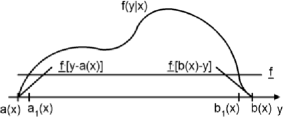
   Figure 2: Approximation of densities with bounded support by $\mathcal{M}_{4}$.

   $f(y|x)\geq\underline{f}\cdot[y-a(x)]^{n}$ on $(a(x),a_{1}(x))$, and $f(y|x)\geq\underline{f}\cdot[b(x)-y]^{n}$ on $(b_{1}(x),b(x))$. Figure 2 provides an illustration for $n=1$.

4. There exists $r>0$ such that $f(\cdot|x)$ is nondecreasing on $(a(x),a_{1}(x)+r/2)$ and nonincreasing on $(b_{1}(x)-r/2,b(x))$ for all $x\in X$.

Then for $\mathcal{M}_{4}$ constructed so that $p_{m}=1/m$, $A_{0}^{m}=\varnothing$, $\mu_{j}^{m}(x)\in A_{j}^{m}(x)$ and $\sigma_{m}(x)=p_{m}^{1/[4(n+1)]}$ and $\sigma_{0}(x)=2(2\pi)^{-1/2}\cdot r$ are independent of $x$, $d_{\mathrm{KL}}(F$,$\mathcal{M}_{4})\rightarrow 0$.

Corollary 5.2.

Assume conditions from Corollary 5.1, $F^{-1}(p|x)$ is continuous in $x$ for all $p\in[0,1]$, $X$ is compact. Then there exists a sequence of polynomials $P_{j}^{m}(x)$ such that $d_{\mathrm{KL}}(F,\mathcal{M}_{5})\rightarrow 0$ where

$$p(y|x,\mathcal{M}_{5})=\sum_{j=1}^{m}p_{m}\phi(y,P_{j}^{m}(x),p_{m}^{1/8}).$$

Let $\mu_{j}^{m}(x)=F^{-1}((j-1/2)p_{m}|x)$. Note that $\mu_{j}^{m}(x)\in A_{j}^{m}(x)=[F^{-1}((j-1)p_{m}|x),F^{-1}(jp_{m}|x)]$ and

$$p_{m}/2=\int_{\mu_{j}^{m}(x)}^{F^{-1}(jp_{m}|x)}f(y|x)\,dy\leq\bigl{(}F^{-1}(jp_{m}|x)-\mu_{j}^{m}(x)\bigr{)}\overline{f}.$$

Similarly, $p_{m}/2\leq(\mu_{j}^{m}(x)-F^{-1}((j-1)p_{m}|x))\overline{f}$. Thus, for $\varepsilon_{m}=p_{m}/(2\overline{f})$, $(\mu_{j}^{m}(x)-\varepsilon_{m},\mu_{j}^{m}(x)+\varepsilon_{m})\subset A_{j}^{m}(x)$. By the Stone–Weierstrass theorem there exist finite order polynomials in $x$, $P_{j}^{m}(x)$ such that $|P_{j}^{m}(x)-\mu_{j}^{m}(x)|<\varepsilon_{m}$. Therefore, $P_{j}^{m}(x)\in A_{j}^{m}(x)$, which was the only requirement on the means of the mixture components in Corollary 5.1.

Example 5.1.

Exponential distribution, $f(y|x)=\gamma(x)\exp\{-\gamma(x)y\}$,$\gamma(x)\geq\underline{\gamma}>0$, $\gamma(x)$ is continuous, $\int\gamma\,dF<\infty$ and the second moment of $y$ is finite ($\int\gamma^{-2}\,dF<\infty$). The quantile function is given by $F^{-1}(p|x)=-\gamma(x)^{-1}\log(1-p)$. Let the partition be such that $A_{0}^{m}=[F^{-1}(mp_{m}|x),\infty)$. Since the exponential density is decreasing the largest interval in the fine part of the partition is given by $A_{m}^{m}=[F^{-1}((m-1)p_{m}|x),F^{-1}(mp_{m}|x))$. Therefore, $h_{m}(x)=h_{m}=\underline{\gamma}^{-1}\log(1+p_{m}/(1-p_{m}m))$. Choosing $p_{m}=(m-m^{0.5})/m^{2}$ guarantees that $h_{m}\rightarrow 0$. For $\sigma_{m}=h_{m}^{1/4}$, and $\delta_{m}(x)=h_{m}^{1/8}$, and $r(x)=1$ conditions (5), (33) and (35) hold.

Next, let $C(1,y,x)=[y,y+1]$ if $y\in[0,1/2]$, $C(1,y,x)=[y-1/2,y+1/2]$ if $y\in[1/2,\infty)$. Since

$$\inf_{z\in C(1,y,x)}f(z|x)\geq\gamma(x)\exp\{-\gamma(x)(y+1)\},$$

we have

$$1\leq f(y|x)\big{/}\inf_{z\in C(1,y,x)}f(z|x)\leq\exp\{\gamma(x)\}.$$

Inequality (34) is satisfied since $\gamma(x)$ is assumed to be integrable. Finally, let $\sigma_{0}(x)=2(2\pi)^{-1/2}$ so that equation (36) in Assumption 5.1 holds. Then,

$$\biggl{|}\int\log[\phi(y,0,\sigma_{0}(x))r(x)/2]F(dy,dx)\biggr{|}=\biggl{|}\int\biggl{[}-\log(4)-\frac{y^{2}\pi}{4}\biggr{]}F(dy,dx)\biggr{|}<\infty$$

since the second moment of $y$ is assumed to be finite. Thus, condition 6 of Assumption 5.1 holds.

If $X$ is compact the same argument as in the proof of Corollary 5.2 can be used to show that $\mu_{j}^{m}(x)$ can be polynomial in $x$ [for fixed $m$ there exists $\varepsilon_{m}>0$ such that $\lambda(A_{j}^{m}(x))>\varepsilon_{m}$ for all $x$ and $j$].

It is possible to give sufficient conditions for approximation results when $\gamma(x)$ is not bounded away from zero, for example, let $r(x)=\gamma(x)^{-1}$, $h_{m}(x)=\gamma(x)^{-1}\log(1+p_{m}/(1-p_{m}m))$, etc. However, then $\sigma_{m}$ and $\sigma_{0}$ would have to be functions of $x$ [not necessarily flexible functions of $x$ but functions that would have the same order as $\gamma(x)$]. Also, $\gamma(x)^{-1}$ is not continuous and the argument I use for justifying the use of polynomial $\mu_{j}^{m}(x)$ breaks down in this case.

Example 5.2.

Uniform distribution, $f(y|x)=b(x)^{-1}1_{[0,b(x)]}(y)$, $b(x)>0$ is continuous, $\int\log b\,dF<\infty$ and the second moment of $y$ is finite ($\int b^{2}\,dF<\infty$). This example demonstrates that the support of $f(y|x)$ does not have to be (un)bounded uniformly in $x$ as long as normal variances are modeled as flexible functions of $x$.

Let the partition be such that $A_{0}^{m}=\varnothing$ and $p_{m}=F(A_{j}^{m}|x)=m^{-1}$, $j>0$. Note that $h_{m}(x)=b(x)/m$. For $\sigma_{m}(x)=b(x)p_{m}^{1/4}$, and $\delta_{m}(x)=b(x)p_{m}^{1/8}$, and $r(x)=b(x)$ conditions (5), (33) and (35) hold.

Next, let $C(r(x),y,x)=[0,b(x)]$. Note that $f(y|x)/\inf_{z\in C(r(x),y,x)}f(z|x)=1$, and inequality (34) is satisfied. Finally, let $\sigma_{0}(x)=2(2\pi)^{-1/2}b(x)$ so that inequality (36) in Assumption 5.1 holds. Then,

$$\biggl{|}\int\log[\phi(y,0,\sigma_{0}(x))r(x)/2]F(dy,dx)\biggr{|}=|{{-}\log(4)-\pi/(3\cdot 4)}|<\infty$$

and condition 6 of Assumption 5.1 holds.

If $X$ is compact and $b(x)$ is bounded away from zero then the same argument, as in the proof of Corollary 5.2, can be used to show that $\mu_{j}^{m}(x)$ can be polynomial in $x$ [for fixed $m$ there exists $\varepsilon_{m}>0$ such that $\lambda(A_{j}^{m}(x))>\varepsilon_{m}$ for all $x$ and $j$].

Corollary 5.3.

Suppose conditions of Proposition 5.1 are satisfied for $h_{m}(x)=h_{m}$, $\sigma_{m}(x)=\sigma_{m}$, $\delta_{m}(x)=\delta_{m}$ and $r(x)=r$ that do not depend on $x$. Also, suppose conditions from parts (i) and (ii) of Corollary 2.1 hold. Then for all sufficiently large $m$,

$$d_{\mathrm{KL}}(F,\mathcal{M}_{4}) \leq \delta_{m}\cdot\frac{d^{1/2}}{2}\int\sup_{z\in C_{\delta_{m}}(y)}\biggl{\|}\frac{d\log f(z|x)}{dz}\biggr{\|}F(dy,dx)$$ (40)

$${}+2\frac{3h_{m}}{(2\pi)^{1/2}\sigma_{m}}+2\exp\biggl{\{}-\frac{(\delta_{m}/\sigma_{m})^{2}}{8}\biggr{\}}$$

$${}+\frac{r}{2}\int_{B_{\delta_{m}}(A_{0}^{m}(x))}\sup_{z\in C_{r}(y)}\biggl{\|}\frac{d\log f(z|x)}{dz}\biggr{\|}F(dy,dx)$$

$${}+\int_{B_{\delta_{m}}(A_{0}^{m}(x))}\biggl{[}\frac{y^{\prime}y}{2\sigma_{0}^{2}}-\log\frac{(r/2)}{(2\pi\sigma_{0}^{2})^{1/2}}\biggr{]}F(dy,dx),$$

where $B_{\delta_{m}}(A_{0}^{m}(x))=\{(y,x,)\dvtx C_{\delta_{m}}(y)\cap A_{0}^{m}(x)\neq\varnothing\}$and bounds in (40)–(40) converge to zero as $m\rightarrow\infty$.

The proof is identical to the proof of Corollary 2.1.

The bounds for $\mathcal{M}_{4}$, (40)–(40), are almost the same as the bounds for $\mathcal{M}_{0}$, (15)–(15), obtained in Corollary 2.1, except for a difference between $B_{\delta_{m}}(A_{0}^{m}(x))$ in $\mathcal{M}_{4}$ and $B_{\delta_{m}}(A_{0}^{m})$ in $\mathcal{M}_{0}$. For the same value of $h_{m}$, the length of the complement of $A_{0}^{m}(x)$ in $\mathcal{M}_{4}$ is bounded above by $mh_{m}$ [$h_{m}=\max_{j>0}\lambda(A_{j}^{m}(x))$] which is the length of the complement of $A_{0}^{m}$ in $\mathcal{M}_{0}$. Thus the bounds obtained for $\mathcal{M}_{4}$ are likely to be larger than the bounds obtained for $\mathcal{M}_{0}$. Compact and interpretable conditions sufficient for deriving an explicit approximation rate for $\mathcal{M}_{4}$ from (40)–(40) seem to be difficult to find. Instead, I show in the following example that not only bounds for $\mathcal{M}_{0}$ can be smaller but also that convergence for $\mathcal{M}_{0}$ can be slightly faster than for $\mathcal{M}_{4}$.

Example 5.3.

Laplace distribution, $f(y|x)=0.5\gamma(x)\exp\{-\gamma(x)|y|\}$,$\gamma(x)\geq\underline{\gamma}>0$, $\gamma(x)$ is continuous, $\int\gamma\,dF<\infty$ and the second moment of $y$ is finite ($\int\gamma^{-2}\,dF<\infty$). Note that nondifferentiability of $f(y|x)$ at zero does not affect any of the theoretical results above.

First consider $\mathcal{M}_{4}$. Let $A_{j}^{m}(x)=[F^{-1}((1-p_{m}m)/2+(j-1)p_{m}|x),F^{-1}((1-p_{m}m)/2+jp_{m}|x))$. Note that $F^{-1}(p|x)=\log(2p)/\gamma(x)$ for $p<0.5$ and $F^{-1}(p|x)=-\log(2(1-p))/\gamma(x)$ for $p\geq 0.5$. Then,

$$h_{m} \geq F^{-1}\bigl{(}(1-p_{m}m)/2+p_{m}|x\bigr{)}-F^{-1}\bigl{(}(1-p_{m}m)/2|x\bigr{)}$$

$$= \frac{1}{\gamma(x)}\log\biggl{(}1+\frac{2p_{m}}{1-p_{m}m}\biggr{)}.$$

Since $h_{m}\rightarrow 0$ and $mp_{m}\rightarrow 1$ we can write

$$p_{m}=\frac{1}{m+g(m)},$$

where $g(m)$ satisfies $g(m)/m\rightarrow 0$ and $g(m)\rightarrow\infty$. Note that

$$B_{\delta_{m}}(A_{0}^{m}(x))\subset\biggl{(}-\infty,\frac{\log(1-p_{m}m)(1-\varepsilon_{0})}{\gamma(x)}\biggr{)}\cup\biggl{(}-\frac{\log(1-p_{m}m)(1-\varepsilon_{0})}{\gamma(x)},\infty\biggr{)}$$

for any $\varepsilon_{0}\in(0,1)$ and all sufficiently large $m$. A direct calculation shows that integrals in (40) and (40) can be bounded by

$$\mbox{constant}\cdot(1-p_{m}m)^{1-\varepsilon}\leq\mbox{constant}\cdot\bigl{(}g(m)/m\bigr{)}^{1-\varepsilon}$$

for any $\varepsilon\in(\varepsilon_{0},1)$ and all sufficiently large $m$. From (5.3) and the mean value theorem,

$$h_{m}\geq\mbox{constant}\cdot\gamma(x)^{-1}\cdot g(m)^{-1}.$$

Since the approximation error bounds increase in $h_{m}$, we should choose the smallest possible value for $h_{m}=\mbox{constant}\cdot\underline{\gamma}^{-1}\cdot g(m)^{-1}$. One can verify that the smallest upper bound for $\delta_{m}$, $h_{m}/\sigma_{m}$, $\exp\{-(\delta_{m}/\sigma_{m})^{2}/8\}$ and $(g(m)/m)^{1-\varepsilon}$ is inside the interval $(m^{-1/3},m^{-1/[3+\varepsilon_{1}]}]$ for any $\varepsilon_{1}>0$ and all sufficiently large $m$. Thus,

$$d_{\mathrm{KL}}(F,\mathcal{M}_{4})\leq\mbox{constant}\cdot\biggl{(}\frac{1}{m}\biggr{)}^{1/[3+\varepsilon_{1}]}.$$

Next, consider $\mathcal{M}_{0}$. Expressions (15) and (15) are exponentially decreasing in $h_{m}m$. Setting $h_{m}$ to a power of $m$, one can show that

$$d_{\mathrm{KL}}(F,\mathcal{M}_{0})\leq\mbox{constant}\cdot\biggl{(}\frac{1}{m}\biggr{)}^{1/[2+\varepsilon_{2}]},$$

for any $\varepsilon_{2}>0$ and all sufficiently large $m$. These results suggest that $\mathcal{M}_{0}$ converges to the target density faster than $\mathcal{M}_{4}$.

It might be unfair to compare approximation errors for $\mathcal{M}_{0}$ and $\mathcal{M}_{4}$. Although both models are “infeasible” and include $m$ functions that need to be approximated by polynomials (or splines), the error from approximation by the polynomials enters the total approximation error in different ways. Nevertheless, the results obtained in this section do seem to suggest that models in which mixing probabilities depend on covariates might perform better in practice.

6 Comparison with Jiang and Tanner (1999)

Jiang and Tanner (1999) is the only work on approximation of conditional densities by ME that I am aware of. Jiang and Tanner (1999) develop approximation and estimation results for target densities of the form

$$\pi(y|x;h(\cdot))=\exp\bigl{(}a(h(x))y+b(h(x))+c(y)\bigr{)}.$$ (42)

Functions $a$, $b$ and $c$ are assumed to be known, $a$ and $b$ are assumed to have nonzero derivatives and $h(x)$ is assumed to have uniformly bounded continuous second order derivatives. It seems that their results could still hold if $a$, $b$ and $c$ are known only up to some parameters (see their Remark 4). Jiang and Tanner (1999) show that $\pi(y|x;h(\cdot))$ can be approximated in the KL distance by ME of the form

$$\sum_{j=1}^{m}\alpha_{j}^{m}(x)\pi(y|x;h_{j}(\cdot)),$$ (43)

where $\pi(\cdot|\cdot;\cdot)$ is defined in (42), $h_{j}(x)$ is a linear function of $x$ and the mixing probabilities $\alpha_{j}^{m}(x)$ can be modeled by logit (more general specifications for mixing weights are also allowed). The idea of their argument is to divide $X$ into a fine partition $B_{j}^{m}$, approximate $1_{B_{j}^{m}}(x)$ by $\alpha_{j}^{m}(x)$ and approximate $h(x)$ by linear function $h_{j}(x)$ on $B_{j}^{m}$. Jiang and Tanner (1999) prove that for their target class of densities a bound on the approximation error is proportional to $m^{-4/d_{x}}$.

There are several important differences between the present work and Jiang and Tanner (1999). First, I consider multivariate responses, $y$, while Jiang and Tanner (1999) consider univariate responses. Most importantly, I do not assume that functional form of $f(y|x)$ is known, for example, known $\pi$, $a$, $b$ and $c$. The components of the model I employ, for example, normal densities and logit mixing probabilities, are generally not related to the true density. As Examples 2.2 and 2.3 and Corollary 5.1 illustrate, many densities that are not from (42) are shown to be approximable by ME models. Examples 2.1 and 5.1 also show that some of the densities from class (42) satisfy sufficient conditions for approximation results I obtain. However, there might exist densities from (42) that violate these sufficient conditions. This would not be surprising since the “correct” functional forms are mixed in (43). For the same reason it is not surprising that the approximation rate obtained by Jiang and Tanner (1999), $m^{-4/d_{x}}$, differs from the ones obtained here, for example, $m^{-1/[d_{x}+2+1/(q-2)+\varepsilon]}$ for model $\mathcal{M}_{3}$ in Corollary 4.1.

Finally, responses in Jiang and Tanner (1999) class (42) can be discrete, for example, Poisson. To accommodate discrete responses in the framework of the present paper one could map the discrete values of response $y$ into a partition of $R$ and introduce a corresponding latent variable $y^{*}\sim p(y^{*}|x,\mathcal{M})$. For example, for binary $y\in\{0,1\}$ let $y^{*}\in(-\infty,0)$ if $y=0$ and $y^{*}\in[0,\infty)$ if $y=1$. Any discrete distribution can be represented by a continuously distributed latent variable in this fashion. This continuous distribution can be flexibly modeled by $p(y^{*}|x,\mathcal{M})$. Models with latent variables are easy to estimate in the Bayesian framework using MCMC methods [see, e.g., Tanner and Wong (1987) and Albert and Chib (1993)].

7 Discussion

This paper shows that large classes of conditional densities can be approximated in the Kullback–Leibler distance by different specifications of finite smooth mixtures of normal densities or regressions. The theory can be generalized to smooth mixtures of location scale densities. These results have interesting implications for applied researchers.

First of all, smooth mixtures of densities or experts can be used as flexible models for estimation of multivariate conditional densities. It seems this issue has not been explored in the literature and it would be interesting to see how specifications studied in the paper work in these settings.

Second, smooth mixtures of simple components, for example, models in which mixing probabilities are modeled by multinomial logit linear in covariates and the means and variances do not depend on covariates, can be quite flexible. A simulation study in Villani, Kohn and Giordani (2009) suggests though that models with more complex components perform better in practice. This issue should be further explored in simulation studies.

Third, results in Section 4 suggest that making mixing probabilities more flexible, for example, by using polynomials in logit, might reduce the number of necessary mixture components. However, these models are more difficult to estimate.

Fourth, models in which mixing probabilities do not depend on covariates can be very flexible at least for univariate response variables. However, they seem to require a lot of mixture components and very flexible models for the means of the mixed normals. Also, approximation error bounds and convergences rates (Example 5.3) obtained in Section 5 suggest that models with flexible mixing probabilities might perform better in practice than models with flexible means of the mixed normals and constant mixing probabilities. Nevertheless, it would be interesting to see how these specifications perform in actual applications and simulation studies.

On the basis of a simulation study, Villani, Kohn and Giordani (2009) generally recommend using heteroscedastic experts (mixture components with variances that depend on covariates). The theory obtained here suggests that heteroscedastic experts might be necessary when differences in quantiles of $f(\cdot|x)$ are not uniformly bounded in $x$ and, especially, when the support bounds of $f(\cdot|x)$ are increasing without a bound in $x$ (see Examples 2.4 and 5.2). This suggestion is likely to remain useful when the differences in quantiles and/or support of $f(\cdot|x)$, although bounded, still change considerably with covariates.

Practical implications of the theoretical results obtained in the paper and summarized in this section are deduced under the assumption of no estimation and parameter uncertainty. Exploring the behavior of the estimation error in addition to the approximation error would result in a more complete understanding of the ME models. This issue is left for future work.

Overall, the paper provides a number of encouraging approximation results for (smooth) mixtures of densities or experts which might stimulate more theoretical and applied work in this area of research.

Appendix

Proof of Proposition 2.1 Since $d_{\mathrm{KL}}$ is always nonnegative,

$$0\leq\int\log\frac{f(y|x)}{p(y|x,\mathcal{M}_{0})}F(dy,dx)\leq\int\log\max\biggl{\{}1,\frac{f(y|x)}{p(y|x,\mathcal{M}_{0})}\biggr{\}}F(dy,dx).$$

Thus, it suffices to show that the last integral in the inequality above converges to zero as $m$ increases. The dominated convergence theorem (DCT) is used for that. First, I establish conditions for point-wise convergence of the integrand to zero a.s. $F$. Then, I present conditions for existence of an integrable upper bound on the integrand required by the DCT.

For fixed $(y,x)$,

$$p(y|x,\mathcal{M}_{0}) = \sum_{j=1}^{m}F(A_{j}^{m}|x)\phi(y,\mu_{j}^{m},\sigma_{m})+F(A_{0}^{m}|x)\phi(y,0,\sigma_{0})$$

$$\geq \inf_{z\in C_{\delta_{m}}(y)}f(z|x)\sum_{j\dvtx A_{j}^{m}\subset C_{\delta_{m}}(y)}\lambda(A_{j}^{m})\phi(y,\mu_{j}^{m},\sigma_{m}),$$

where $\lambda$ is the Lebesgue measure.

In Lemmas .1 and .2, I derive the following bounds for the Riemann sum in (Appendix) (the Riemann sum is not far from the corresponding normal integral, and the integral is not far from 1):

$$\sum_{j\dvtx A_{j}^{m}\subset C_{\delta_{m}}(y)}\lambda(A_{j}^{m})\phi(y,\mu_{j}^{m},\sigma_{m})$$

$$\qquad\geq 1-\frac{3d^{3/2}\delta_{m}^{d-1}h_{m}}{(2\pi)^{d/2}\sigma_{m}^{d}}-\frac{8(\sigma_{m}/\delta_{m})}{(2\pi)^{1/2}}\exp\biggl{\{}-\frac{(\delta_{m}/\sigma_{m})^{2}}{8}\biggr{\}}$$ (45)

$$\qquad\geq 1-\frac{3d^{3/2}\delta_{m}^{d-1}h_{m}}{(2\pi)^{d/2}\sigma_{m}^{d}}-\exp\biggl{\{}-\frac{(\delta_{m}/\sigma_{m})^{2}}{8}\biggr{\}},$$

where the last inequality holds for all sufficiently large $m$ ($\delta_{m}/\sigma_{m}\rightarrow\infty$). Given $\varepsilon>0$ there exists $M_{1}$ such that for $m\geq M_{1}$, expressions in (Appendix) are bounded below by $(1-\varepsilon)$.

If $f(y|x)$ is continuous in $y$ at $(y,x)$ and $f(y|x)>0$ there exists $M_{2}$ such that for $m\geq M_{2}$, $[f(y|x)/\inf_{z\in C_{\delta_{m}}(y)}f(z|x)]\leq(1+\varepsilon)$ since $\delta_{m}\rightarrow 0$. For any $m\geq\max\{M_{0},M_{1},M_{2}\}$,

$$1 \leq \max\biggl{\{}1,\frac{f(y|x)}{p(y|x,\mathcal{M}_{0})}\biggr{\}}$$

$$\leq \max\biggl{\{}1,\frac{f(y|x)}{\inf_{z\in C_{\delta_{m}}(y)}f(z|x)(1-\varepsilon)}\biggr{\}}\leq\frac{1+\varepsilon}{1-\varepsilon}.$$

Thus, $\log\max\{1,f(y|x)/p(y|x,\mathcal{M}_{0})\}\rightarrow 0$ a.s. $F$ as long as $f(y|x)$ is continuous in $y$ a.s. $F$ [$f(y|x)$ is always positive a.s. $F$].

Parts 2 and 3 of Assumption 2.1 are used for establishing an integrable upper bound for the DCT

$$p(y|x,\mathcal{M}_{0}) = \sum_{j=1}^{m}F(A_{j}^{m}|x)\phi(y,\mu_{j}^{m},\sigma_{m})+F(A_{0}^{m}|x)\phi(y,0,\sigma_{0})$$

$$\geq [1-1_{A_{0}^{m}}(y)]$$

$${}\times\inf_{z\in C_{1}(r,y,x)}f(z|x)\cdot\sum_{j\dvtx A_{j}^{m}\subset C_{1}(r,y,x)}\lambda(A_{j}^{m})\phi(y,\mu_{j}^{m},\sigma_{m})$$

$${}+1_{A_{0}^{m}}(y)\cdot\inf_{z\in C_{0}(r,y,x)}f(z|x)\cdot\lambda(C_{0}(r,y,x))\phi(y,0,\sigma_{0}).$$

Lemmas .1 and .2 imply that the Riemann sum in (Appendix) is bounded below by $2^{-d}-2^{-(d+1)}=2^{-(d+1)}$ for any $m$ larger then some $M_{4}$. Inequalities (Appendix) and (5) imply

$$\log\max\biggl{\{}1,\frac{f(y|x)}{p(y|x,\mathcal{M}_{0})}\biggr{\}}$$

$$\qquad\leq\log\max\biggl{\{}1,\frac{f(y|x)}{\inf_{z\in C(r,y,x)}f(z|x)\cdot\phi(y,0,\sigma_{0})\cdot(r/2)^{d}}\biggr{\}}$$

$$\qquad=\log\frac{1}{\phi(y,0,\sigma_{0})(r/2)^{d}}\max\biggl{\{}\phi(y,0,\sigma_{0})(r/2)^{d},\frac{f(y|x)}{\inf_{z\in C(r,y,x)}f(z|x)}\biggr{\}}$$

$$\qquad\leq-\log\bigl{(}\phi(y,0,\sigma_{0})(r/2)^{d}\bigr{)}+\log\frac{f(y|x)}{\inf_{z\in C(r,y,x)}f(z|x)},$$

where inequality (Appendix) follows by the first inequality in (5). The first expression in (Appendix) is integrable by Assumption 2.1, part 2. The second expression in (Appendix) is integrable by Assumption 2.1, part 3. Thus the proposition is proved. Proof of Corollary 2.1 The proof of the first part of the proposition is a simple implication of the argument in the proof of Proposition 2.1. Note that

$$d_{\mathrm{KL}}(F,\mathcal{M}_{0}) = \int_{Y\times X\setminus B_{\delta_{m}}(A_{0}^{m})}\log\frac{f(y|x)}{p(y|x,\mathcal{M}_{0})}F(dy,dx)$$

$${}+\int_{B_{\delta_{m}}(A_{0}^{m})}\log\frac{f(y|x)}{p(y|x,\mathcal{M}_{0})}F(dy,dx).$$

For $(y,x)\in Y\times X\setminus B_{\delta_{m}}(A_{0}^{m})$, inequalities (Appendix) and (Appendix) apply. Thus, the first integral in (Appendix) is bounded by the sum of (10) and (10), where the bound in (10) is obtained by the mean value theorem for $-\log(1-x)$ and a small positive $x$,

$$-\log\biggl{(}1-\frac{3d^{3/2}\delta_{m}^{d-1}h_{m}}{(2\pi)^{d/2}\sigma_{m}^{d}}-\exp\biggl{\{}-\frac{(\delta_{m}/\sigma_{m})^{2}}{8}\biggr{\}}\biggr{)}$$

(49)

$$\qquad\leq 2\biggl{(}\frac{3d^{3/2}\delta_{m}^{d-1}h_{m}}{(2\pi)^{d/2}\sigma_{m}^{d}}+\exp\biggl{\{}-\frac{(\delta_{m}/\sigma_{m})^{2}}{8}\biggr{\}}\biggr{)}.$$

By inequality (Appendix), the second integral in (Appendix) is bounded by the sum of (10) and (10).

Expression (10) converges to zero by the DCT. The point-wise convergence follows by the assumed continuity and positivity of $f(y|x)$. An integrable upper bound is given by (4). Expression (10) converges to zero by (3). Expressions (10) and (10) converge to zero because $Y\times X\setminus B_{\delta_{m}}(A_{0}^{m})\nearrow Y\times X$ and the integrands are integrable by (4) and by the assumed finiteness of the second moment of $y$. Thus, the first part of the proposition is proved.

The second part of the proposition [bounds for differentiable $f(y|x)$] follows from the first part since

$$\biggl{|}\log\frac{f(y|x)}{\inf_{z\in C_{r}(y)}f(z|x)}\biggr{|}\leq\sup_{z\in C_{r}(y)}\biggl{\|}\frac{d\log f(z|x)}{dz}\biggr{\|}\frac{d^{1/2}r}{2},$$

which is implied by the multivariate mean value theorem: for any $(z_{1},z_{2})$

$$|{\log f(z_{1}|x)-\log f(z_{2}|x)}|\leq\bigl{\|}f^{\prime}\bigl{(}cz_{1}+(1-c)z_{2}\bigr{)}\bigr{\|}\|z_{1}-z_{2}\|$$

for some $c\in[0,1]$. Convergence of the bounds to zero is obtained in the same way as in the first part of the proposition.

To obtain the third part let us suppose that the fine part of the partition $\{A_{j}^{m},1\leq j\leq m\}$ is centered at 0. If $(y,x)\in B_{\delta_{m}}(A_{0}^{m})$, then $|y_{i}|\geq h_{m}m^{1/d}/2-\delta_{m}>h_{m}m^{1/d}/3$ for $i\in\{1,\ldots,d\}$ and all sufficiently large $m$ and

$$\int_{B_{\delta_{m}}(A_{0}^{m})}y_{i}^{2}F(dy,dx)$$

$$\qquad\leq\int_{\{(y,x)\dvtx|y_{i}|>h_{m}m^{1/d}/3,\forall i\}}y_{i}^{2}F(dy,dx)$$

$$\qquad\leq(h_{m}m^{1/d}/3)^{-(q-2)}$$

$$\qquad\quad{}\times\int_{\{(y,x)\dvtx|y_{i}|>h_{m}m^{1/d}/3,\forall i\}}(h_{m}m^{1/d}/3)^{q-2}y_{i}^{2}F(dy,dx)$$

$$\qquad\leq(h_{m}m^{1/d}/3)^{-(q-2)}\int_{Y\times X}y_{i}^{q}F(dy,dx).$$

Similarly,

$$\int_{B_{\delta_{m}}(A_{0}^{m})}\sup_{z\in C_{r}(y)}\biggl{\|}\frac{d\log f(z|x)}{dz}\biggr{\|}F(dy,dx)$$

$$\qquad\leq\int_{\{(y,x)\dvtx|y_{i}|>h_{m}m^{1/d}/3,\forall i\}}\sup_{z\in C_{r}(y)}\biggl{\|}\frac{d\log f(z|x)}{dz}\biggr{\|}F(dy,dx)$$

$$\qquad\leq\biggl{(}\int_{\{(y,x)\dvtx|y_{i}|>h_{m}m^{1/d}/3,\forall i\}}(h_{m}m^{1/d}/3)^{q-2}$$

$$\hskip 137.0pt{}\times\sup_{z\in C_{r}(y)}\biggl{\|}\frac{d\log f(z|x)}{dz}\biggr{\|}F(dy,dx)\biggr{)}$$

$$\qquad\quad{}\times\bigl{(}(h_{m}m^{1/d}/3)^{q-2}\bigr{)}^{-1}$$

$$\qquad\leq(h_{m}m^{1/d}/3)^{-(q-2)}\int_{Y\times X}y_{i_{1}}^{q-2}\sup_{z\in C_{r}(y)}\biggl{\|}\frac{d\log f(z|x)}{dz}\biggr{\|}F(dy,dx).$$

Since integrals in (Appendix) and (Appendix) are finite by assumption, (15) and (15) can be bounded above by an expression proportional to $(h_{m}m^{1/d})^{-(q-2)}$. Thus, the sum of (15)–(15) is bounded by

$$c_{1}\cdot\delta_{m}+c_{2}\cdot\exp\{-(\delta_{m}/\sigma_{m})^{2}/8\}+c_{3}\cdot\delta_{m}^{d-1}h_{m}/\sigma_{m}^{d}$$

(52)

$$\qquad{}+c_{4}\cdot 1/(h_{m}m^{1/d})^{q-2},$$

where constants $c_{1}$, $c_{2}$, $c_{3}$ and $c_{4}$ do not depend on $m$. Let $b_{m}$ be the smallest number satisfying $b_{m}\geq\delta_{m}$, $b_{m}\geq\delta_{m}^{d-1}h_{m}/\sigma_{m}^{d}$, $b_{m}\geq 1/(h_{m}m^{1/d})^{q-2}$ and $b_{m}\geq\exp\{-(\delta_{m}/\sigma_{m})^{2}/8\}$. The first three of these inequalities imply

$$b_{m}\geq\{[(\delta_{m}/\sigma_{m})^{d}]/m^{1/d}\}^{1/[2+1/(q-2)]}.$$

It implies that for all sequences $\delta_{m}$, $\sigma_{m}$ and $h_{m}$ allowed by the corollary,

$$b_{m}>\biggl{(}\frac{1}{m}\biggr{)}^{1/(d\cdot[2+1/(q-2)])}.$$

One can verify that

$$\qquad b_{m}\leq\biggl{(}\frac{(4\log m/d)^{d/2}}{m^{1/d}}\biggr{)}^{1/[2+1/(q-2)]}\leq\biggl{(}\frac{1}{m}\biggr{)}^{1/(d\cdot[2+1/(q-2)+\varepsilon])},$$ (53)

when $\delta_{m}$ equal to the first bound in (53), $(\delta_{m}/\sigma_{m})^{2}=4\log m/d$ and $h_{m}=\delta_{m}^{2}/(\delta_{m}/\sigma_{m})^{d}$. Proof of Proposition 4.1 Define $I_{1}^{m}(x,s_{m})=\{i\dvtx\|x_{i}^{m}-x\|^{2}<s_{m}\}$ and $I_{2}^{m}(x,s_{m})=\{i\dvtx\|x_{i}^{m}-x\|^{2}>2s_{m}\}$. For $i\in I_{1}^{m}(x,s_{m})$,

$$[-R_{m}(x_{i}^{m\prime}x_{i}^{m}-2x_{i}^{m\prime}x)]>[-R_{m}(s_{m}-x^{\prime}x)]$$ (54)

and for $i\in I_{2}^{m}(x,s_{m})$,

$$[-R_{m}(x_{i}^{m\prime}x_{i}^{m}-2x_{i}^{m\prime}x)]<[-R_{m}(2s_{m}-x^{\prime}x)].$$ (55)

Note that

$$\frac{\sum_{i\in I_{1}^{m}(x,s_{m})}\exp\{-R_{m}(x_{i}^{m\prime}x_{i}^{m}-2x_{i}^{m\prime}x)\}}{\sum_{l}\exp\{-R_{m}(x_{l}^{m\prime}x_{l}^{m}-2x_{l}^{m\prime}x)\}}$$

$$\qquad\geq 1-\frac{\sum_{i\in I_{2}^{m}(x,s_{m})}\exp\{-R_{m}(x_{i}^{m\prime}x_{i}^{m}-2x_{i}^{m\prime}x)\}}{\sum_{i\in I_{1}^{m}(x,s_{m})}\exp\{-R_{m}(x_{i}^{m\prime}x_{i}^{m}-2x_{i}^{m\prime}x)\}}$$

$$\qquad\geq 1-\frac{\mbox{card}(I_{2}^{m}(x,s_{m}))}{\mbox{card}(I_{1}^{m}(x,s_{m}))}\exp\{-R_{m}s_{m}\}\geq 1-d_{x}^{d_{x}/2}\frac{\exp\{-R_{m}s_{m}\}}{s_{m}^{d_{x}/2}},$$

where the second inequality follows from (54) and (55). The last inequality follows from the following bounds on the number of elements in $I_{1}^{m}(x,s_{m})$ and $I_{2}^{m}(x,s_{m})$: $\mbox{card}(I_{1}^{m}(x,s_{m}))\geq 1$ [$s_{m}$ is chosen in (22) so that any ball in $X$ with radius $s_{m}^{1/2}$ has to contain at least one $x_{i}^{m}$] and

$$\mbox{card}(I_{2}^{m}(x,s_{m}))\leq N(m)=d_{x}^{d_{x}/2}s_{m}^{-d_{x}/2}.$$

For $i\in I_{1}^{m}(x,s_{m})$ and $A_{j}^{m}\subset C_{\delta_{m}}(y)$,

$$F(A_{j}^{m}|x_{i}^{m})\geq\lambda(A_{j}^{m})\inf_{z\in C_{\delta_{m}}(y),\|t-x\|^{2}\leq s_{m}}f(z|t).$$ (57)

Inequalities (Appendix), (57) and (Appendix) imply that $p(y|x,\mathcal{M}_{3})$ exceeds

$$\sum_{j\dvtx A_{j}^{m}\subset C_{\delta_{m}}(y)}\sum_{i\in I_{1}^{m}(x,s_{m})}F(A_{j}^{m}|x_{i}^{m})\frac{\exp\{-R_{m}(x_{i}^{m\prime}x_{i}^{m}-2x_{i}^{m\prime}x)\}}{\sum_{l}\exp\{-R_{m}(x_{l}^{m\prime}x_{l}^{m}-2x_{l}^{m\prime}x)\}}\phi(y,\mu_{j}^{m},\sigma_{m})$$

$$\qquad\geq\inf_{z\in C_{\delta_{m}}(y),\|t-x\|^{2}\leq s_{m}}f(z|t)\cdot\biggl{[}1-\frac{3d^{3/2}\delta_{m}^{d-1}h_{m}}{(2\pi)^{d/2}\sigma_{m}^{d}}$$

$$\qquad\quad\hskip 120.2pt{}-\frac{8d\sigma_{m}}{(2\pi)^{1/2}\delta_{m}}\exp\biggl{\{}-\frac{(\delta_{m}/\sigma_{m})^{2}}{8}\biggr{\}}\biggr{]}$$

$$\qquad\quad\hskip 78.5pt{}\times\biggl{[}1-d_{x}^{d_{x}/2}\frac{\exp\{-R_{m}s_{m}\}}{s_{m}^{d_{x}/2}}\biggr{]}.$$

The expression on the last line of this inequality converges to $1$ by (22). The rest of the proof is exactly the same as the proof of Proposition 2.1. Proof of Corollary 4.1 The proof of part (i) is identical to the proof of Corollary 2.1 part (ii).

The proof of part (ii) is also similar to the proof of Corollary 2.1 part (iii). Just set $s_{m}^{1/2}=\delta_{m}$ and note that (28) can be made arbitrarily smaller than the other parts of the bound by an appropriate choice of $R_{m}$. Thus, the bound is the same as in (18), we just need to express $m$ in terms of the number of mixture components in $\mathcal{M}_{3}$, $mN(m)$. From the definition of $N(m)$ and $s_{m}$, $N(m)=\lambda(B_{i}^{m})^{-1}=d_{x}^{d_{x}/2}s_{m}^{-d_{x}/2}$. Since we set $s_{m}^{1/2}=\delta_{m}$ and $\delta_{m}=m^{-1/(d\cdot[2+1/(q-2)])}$ in the proof of Corollary 2.1,

$$mN(m)=d_{x}^{d_{x}/2}m^{1+d_{x}/(d\cdot[2+1/(q-2)])}.$$

From this equation, one can express $m$ as a function of $mN(m)$ and plug it in (18) to obtain (31). Proof of Proposition 5.1 First, consider point-wise convergence a.s. $F$. For fixed $(y,x)$ and an interval $C_{\delta_{m}(x)}(y)$ with center $y$ and length $\delta_{m}(x)>0$,

$$\hskip 32.0ptp(y|x,\mathcal{M}_{4}) = \sum_{j=1}^{m}F(A_{j}^{m}(x)|x)\phi(y,\mu_{j}^{m}(x),\sigma_{m}(x))$$

$${}+F(A_{0}^{m}(x)|x)\phi(y,0,\sigma_{0}(x))$$

$$\geq \inf_{z\in C_{\delta_{m}(x)}(y)}f(z|x)\sum_{j=1}^{m}\lambda\bigl{(}A_{j}^{m}(x)\cap C_{\delta_{m}(x)}(y)\bigr{)}$$

$$\hskip 90.1pt{}\times\phi(y,\mu_{j}^{m}(x),\sigma_{m}(x))$$

$$\geq \inf_{z\in C_{\delta_{m}(x)}(y)}f(z|x)\biggl{(}1-\frac{6h_{m}(x)}{(2\pi)^{1/2}\sigma_{m}(x)}$$

$$\hskip 80.38pt{}-\frac{16\sigma_{m}(x)}{(2\pi)^{1/2}\delta_{m}(x)}\exp\biggl{\{}-\frac{(\delta_{m}/\sigma_{m})^{2}}{8}\biggr{\}}\biggr{)},$$

where the last inequality follows from Lemma .3 [if $\delta_{m}(x)\rightarrow 0$ and $mp_{m}\rightarrow 1$ then for any $(y,x)$ there exists $M$ such that $\forall m\geq M$, $C_{\delta_{m}(x)}(y)\cap A_{0}^{m}(x)=\varnothing$ and the lemma applies]. Convergence of the bound in (Appendix) to $f(y|x)$ a.s. $F$ is implied by a.s. positivity and continuity in $y$ of $f(y|x)$ and conditions in (33). The rest of the argument establishing point-wise convergence is the same as for $\mathcal{M}_{0}$ [details are below (3)].

Next, let us derive an integrable upper bound for the DCT,

$$\hskip 28.0ptp(y|x,\mathcal{M}_{4}) = \sum_{j=1}^{m}F(A_{j}^{m}(x)|x)\phi(y,\mu_{j}^{m}(x),\sigma_{m}(x))$$

$${}+F(A_{0}^{m}(x)|x)\phi(y,0,\sigma_{0}(x))$$

$$\geq [1-1_{A_{0}^{m}(x)}(y)]$$

$${}\times\inf_{z\in C_{1}(r(x),y,x)}f(z|x)$$

$$\hskip 66.0pt{}\times\sum_{j\dvtx A_{j}^{m}(x)\subset C_{1}(r(x),y,x)}\lambda(A_{j}^{m}(x))$$

$$\hskip 161.0pt{}\times\phi(y,\mu_{j}^{m}(x),\sigma_{m}(x))$$

$${}+1_{A_{0}^{m}(x)}(y)\cdot\inf_{z\in C_{0}(r(x),y,x)}f(z|x)\cdot\lambda(C_{0}(r(x),y,x))$$

$$\hskip 117.2pt{}\times\phi(y,0,\sigma_{0}(x)).$$

Lemma .3 and condition (35) imply that the sum in (Appendix) is bounded below by $1/2-1/4=1/4$ for all sufficiently large $m$. Equation (36) implies

$$\log\max\biggl{\{}1,\frac{f(y|x)}{p(y|x,\mathcal{M}_{4})}\biggr{\}}$$

$$\qquad\leq\log\max\biggl{\{}1,\frac{f(y|x)\cdot(r(x)/2)^{-1}}{\inf_{z\in C(r(x),y,x)}f(z|x)\cdot\phi(y,0,\sigma_{0}(x))}\biggr{\}}$$

$$\qquad\leq\log\frac{1}{\phi(y,0,\sigma_{0}(x))(r(x)/2)}\max\biggl{\{}\phi(y,0,\sigma_{0}(x))\bigl{(}r(x)/2\bigr{)},$$

$$\hskip 184.0pt\frac{f(y|x)}{\inf_{z\in C(r(x),y,x)}f(z|x)}\biggr{\}}$$

$$\qquad\leq-\log[\phi(y,0,\sigma_{0}(x))r(x)/2]+\log\frac{f(y|x)}{\inf_{z\in C(r(x),y,x)}f(z|x)}.$$

Inequality (Appendix) follows by (36). The first expression in (Appendix) is integrable by Assumption 5.1, part 6. The second expression in (Appendix) is integrable by Assumption 5.1, part 3. This completes the proof of the proposition. Proof of Corollary 5.1 It suffices to show that Assumption 5.1 is satisfied. First, let us obtain a suitable $h_{m}$. Note that

$$\qquad p_{m}\geq\int_{A_{j}^{m}(x)\cap[a_{1}(x),b_{1}(x)]}f(y|x)\,dy\geq\lambda\bigl{(}A_{j}^{m}(x)\cap[a_{1}(x),b_{1}(x)]\bigr{)}\underline{f}.$$ (61)

Also,

$$p_{m} \geq \int_{A_{j}^{m}(x)\cap[a(x),a_{1}(x)]}f(y|x)\,dy$$

$$\geq \int_{A_{j}^{m}(x)\cap[a(x),a_{1}(x)]}\underline{f}\cdot[y-a(x)]^{n}\,dy$$

$$\geq (n+1)^{-1}\lambda\bigl{(}A_{j}^{m}(x)\cap[a(x),a_{1}(x)]\bigr{)}^{n+1}\underline{f}$$

and similarly $p_{m}\geq(n+1)^{-1}\lambda(A_{j}^{m}(x)\cap[b_{1}(x),b(x)])^{n+1}\underline{f}$. Combining this inequality with (61) and (Appendix) we get for all $x$ and $j$,

$$\lambda(A_{j}^{m}(x)) \leq \frac{p_{m}}{\underline{f}}+\frac{2\cdot(n+1)^{1/(n+1)}\cdot p_{m}^{1/(n+1)}}{\underline{f}^{1/(n+1)}}$$

$$\leq \frac{7p_{m}^{1/(n+1)}}{\underline{f}}=h_{m}.$$

For $\sigma_{m}(x)=p_{m}^{1/4(n+1)}$ and $\delta_{m}(x)=p_{m}^{1/8(n+1)}$ conditions (5), (33) and (35) hold.

Next, let $C(r,y,x)=[y,y+r]$ if $y\in(a(x),a_{1}(x)+r/2)$, $C(r,y,x)=[y-r/2,y+r/2]$ if $y\in[a_{1}(x)+r/2,b_{1}(x)-r/2]$ and $C(r,y,x)=[y-r/2,y]$ if $y\in(b_{1}(x)-r/2,b(x))$. By condition 4 of the corollary $\inf_{z\in C(r(x),y,x)}f(z|x)=f(y|x)$ for $y\notin[a_{1}(x)+r/2,b_{1}(x)-r/2]$. For $y\in[a_{1}(x)+r/2,b_{1}(x)-r/2]$, $\inf_{z\in C(r(x),y,x)}f(z|x)\geq\underline{f}$ and

$$\int\log\frac{f(y|x)}{\inf_{z\in C(r(x),y,x)}f(z|x)}F(dy,dx)\leq\log(\overline{f}/\underline{f})<\infty.$$

Condition 2 and (36) in Assumption 5.1 are assumed in the corollary. Since $a(x)$ and $b(x)$ are assumed to be square integrable, the second moment of $y$ is finite, and condition 6 of Assumption 5.1 holds.

Lemma .1.

Define a hypercube $C_{\delta}(y)=\{\mu\in R^{d}\dvtx y_{i}\leq\mu_{i}\leq y_{i}+\delta,i=1,\ldots,d\}$. Let $A_{1},\ldots,A_{m}$ be adjacent hypercubes with centers $\mu_{j}$ and side length $h$ such that $C_{\delta}(y)\subset\bigcup_{j=1}^{m}A_{j}$ and $\delta>3d^{1/2}h$. Define $J=\{j\dvtx A_{j}\subset C_{\delta}(y)\}$. Then

$$\sum_{j\in J}{\lambda(A_{j})\phi(y;\mu_{j},\sigma)}\geq\int_{C_{\delta}(y)}{\phi(\mu;y;\sigma)\,d\mu}-\frac{3d^{3/2}\delta^{d-1}h}{(2\pi)^{d/2}\sigma^{d}}.$$

By symmetry, this result holds for any hypercube with vertex at $y$ and side length $\delta$. This implies that for hypercube $D_{\delta}(y)=\{x\dvtx y_{i}-\delta/2\leq x_{i}\leq y_{i}+\delta/2,i=1,\ldots,d\}$,

$$\sum_{j\dvtx A_{j}\subset D_{\delta}(y)}{\lambda(A_{j})\phi(y;\mu_{j},\sigma)}\geq\int_{D_{\delta}(y)}{\phi(\mu;y;\sigma)\,d\mu}-2^{d}\frac{3d^{3/2}(\delta/2)^{d-1}h}{(2\pi)^{d/2}\sigma^{d}}$$

as long as $D_{\delta}(y)\subset\bigcup_{j=1}^{m}A_{j}$ and $\delta>6d^{1/2}h$.

For $j\in J$ let $B_{j}=\{x\dvtx\mu_{ji}\leq x_{i}\leq\mu_{ji}+h,i=1,\ldots,d\}$ be a shifted and rotated version of $A_{j}$. Note that $\mu_{j}=\arg\max_{\mu\in B_{j}}\phi(\mu;y;\sigma)$, and therefore

$$\sum_{j\in J}{\lambda(A_{j})\phi(y;\mu_{j},\sigma)}$$

$$\qquad=\sum_{j\in J}{\lambda(B_{j})\phi(y;\mu_{j},\sigma)}\geq\int_{\bigcup_{j\in J}B_{j}}{\phi(\mu;y;\sigma)\,d\mu}$$

$$\qquad\geq\int_{C_{\delta}(y)}{\phi(\mu;y;\sigma)\,d\mu}-\int_{C_{\delta}(y)\setminus\bigcup_{j\in J}B_{j}}{\phi(\mu;y;\sigma)\,d\mu}.$$

Since $\{x\dvtx\min_{J}\mu_{ji}\leq x_{i}\leq\max_{J}\mu_{ji},i=1,\ldots,d\}\subset C_{\delta}(y)\cap[\bigcup_{J}B_{j}]$ and $\max_{j\in J}\mu_{ji}-\min_{j\in J}\mu_{ji}\geq\delta-3d^{1/2}h$, we get $\lambda(C_{\delta}(y)\cap[\bigcup_{J}B_{j}])\geq(\delta-3d^{1/2}h)^{d}$ and

$$\lambda\biggl{(}C_{\delta}(y)\Bigm{\backslash}\biggl{[}\bigcup_{J}B_{j}\biggr{]}\biggr{)} = \lambda(C_{\delta}(y))-\lambda\biggl{(}C_{\delta}(y)\cap\biggl{[}\bigcup_{j\in J}B_{j}\biggr{]}\biggr{)}$$

$$\leq \delta^{d}-(\delta-3d^{1/2}h)^{d}\leq 3d^{3/2}h\delta^{d-1},$$

where the last inequality follows by induction. Thus,

$$\int_{C_{\delta}(y)\setminus\bigcup_{J}B_{j}}{\phi(\mu;y;\sigma)\,d\mu} \leq \lambda\biggl{(}C_{\delta}(y)\Bigm{\backslash}\biggl{[}\bigcup_{J}B_{j}\biggr{]}\biggr{)}\frac{1}{(2\pi)^{d/2}\sigma^{d}}$$

$$\leq \frac{3d^{3/2}h\delta^{d-1}}{(2\pi)^{d/2}\sigma^{d}}.$$

Lemma .2.

Let $C_{\delta}(y)$ be a $d$-dimensional hypercube with center $y$ and side length $\delta>0$. Then

$$\int_{C_{\delta}(y)}{\phi(\mu;y;\sigma)\,d\mu}>1-\frac{8d\sigma/\delta}{(2\pi)^{1/2}}\exp\biggl{\{}-\frac{(\delta/\sigma)^{2}}{8}\biggr{\}}.$$

Note that this inequality immediately implies that for any sub-hypercube of $C_{\delta}(y)$, $\tilde{C}$, with vertex at $y$ and side length $\delta/2$, for example, $\tilde{C}=C_{\delta}(y)\cap[\mu\geq y]$,

$$\int_{\tilde{C}}{\phi(\mu;y;\sigma)\,d\mu} = \frac{1}{2^{d}}\int_{C_{\delta}(y)}{\phi(\mu;y;\sigma)\,d\mu}$$

$$> \frac{1}{2^{d}}-\frac{8d\sigma/\delta}{2^{d}(2\pi)^{1/2}}\exp\biggl{\{}-\frac{(\delta/\sigma)^{2}}{8}\biggr{\}}.$$

$$\int_{C_{\delta(y)}}{\phi(\mu;y;\sigma)\,d\mu} = \int_{\bigcap_{i=1}^{d}[|\mu_{i}|\leq\delta/2]}{\phi(\mu;0;\sigma)\,d\mu}$$

$$= 1-\int_{\bigcup_{i=1}^{d}[|\mu_{i}|\geq\delta/2]}{\phi(\mu;0;\sigma)\,d\mu}$$

$$\geq 1-\sum_{i=1}^{d}\int_{|\mu_{i}|\geq\delta/2}{\phi(\mu_{i};0;\sigma)\,d\mu_{i}}$$

$$= 1-2d\int_{\delta/2}^{\infty}{\phi(\mu_{1};0;\sigma)\,d\mu_{1}}$$

$$> 1-\frac{2d}{(2\pi)^{1/2}\sigma}\int_{\delta/2}^{\infty}{\exp\biggl{\{}-\frac{0.5(\delta/2)\mu_{1}}{\sigma^{2}}\biggr{\}}\,d\mu_{1}}$$

$$= 1-\frac{2d}{(2\pi)^{1/2}\sigma}\frac{-\sigma^{2}}{0.5(\delta/2)}\exp\{-0.5(\delta/2)\mu_{1}/\sigma^{2}\}|_{\delta/2}^{\infty}$$

$$= 1-\frac{8d(\sigma/\delta)}{(2\pi)^{1/2}}\exp\biggl{\{}-\frac{(\delta/\sigma)^{2}}{8}\biggr{\}}.$$

Lemma .3.

Let $A_{1},\ldots,A_{m}$ be a partition of an interval on $R$ such that $\lambda(A_{j})\leq h$ and $\mu_{j}\in A_{j}$. Assume $C_{\delta}(y)=[y-\delta,y+\delta]\subset\cup A_{j}$ is an interval with center $y$ and length $\delta$. Then

$$\sum_{j=1}^{m}\lambda\bigl{(}A_{j}\cap C_{\delta}(y)\bigr{)}\phi(y,\mu_{j},\sigma)\geq 1-\frac{6h}{(2\pi)^{1/2}\sigma}-\frac{8(\sigma/\delta)}{(2\pi)^{1/2}}\exp\biggl{\{}-\frac{(\delta/\sigma)^{2}}{8}\biggr{\}}.$$

If $C_{\delta}(y)=[y-\delta,y]$ or $C_{\delta}(y)=[y,y+\delta]$ the lower bound in the above expression should be divided by 2.

Let $J=\{j\dvtx A_{j}\cap C_{\delta}(y)\subset[y-\delta,y]\}$. For any $j\in J$ and $\mu\in A_{j}\cap C_{\delta}(y)$, $\mu-h\leq\mu_{j}$ as $\lambda(A_{j})<h$ and $\mu_{j}\in A_{j}$, which implies $\phi(y,\mu_{j},\sigma)\geq\phi(y,\mu-h,\sigma)$. Therefore,

$$\qquad\sum_{j\in J}\lambda\bigl{(}A_{j}\cap C_{\delta}(y)\bigr{)}\phi(y,\mu_{j},\sigma)\geq\int_{\bigcup_{j\in J}[A_{j}\cap C_{\delta}(y)]}\phi(y,\mu-h,\sigma)\,d\mu.$$ (63)

Note next that

$$\int_{\bigcup_{j\in J}[A_{j}\cap C_{\delta}(y)]}\phi(y,\mu-h,\sigma)\,d\mu$$

$$\qquad\geq\int_{y-\delta}^{y-h}\phi(y,\mu-h,\sigma)\,d\mu=\int_{y-\delta-h}^{y-2h}\phi(y,\mu,\sigma)\,d\mu$$

$$\qquad=\int_{y-\delta}^{y}\phi(y,\mu,\sigma)\,d\mu$$

$$\qquad\quad{}-\int_{y-\delta-h}^{y-\delta}\phi(y,\mu,\sigma)\,d\mu-\int_{y-2h}^{y}\phi(y,\mu,\sigma)\,d\mu$$

$$\qquad\geq\int_{y-\delta}^{y}\phi(y,\mu,\sigma)\,d\mu-\frac{3h}{(2\pi)^{1/2}\sigma}.$$

By symmetry the same results can be obtained for $J=\{j\dvtx A_{j}\cap C_{\delta}(y)\subset[y,y+\delta]\}$. Thus

$$\sum_{j=1}^{m}\lambda\bigl{(}A_{j}\cap C_{\delta}(y)\bigr{)}\phi(y,\mu_{j},\sigma)\geq\int_{y-\delta}^{y+\delta}\phi(y,\mu,\sigma)\,d\mu-2\frac{3h}{(2\pi)^{1/2}\sigma}.$$

The claim of the lemma follows by Lemma .2.

References

Albert and Chib (1993)Albert, J. H. and Chib, S. (1993).
Bayesian analysis of binary and polychotomous response data.
J. Amer. Statist. Assoc.88 669–679.
\MR1224394
Geweke and Keane (2007)Geweke, J. and Keane, M. (2007).
Smoothly mixing regressions.
J. Econometrics138 252–290.
\MR2380699
Ghosh and
Ramamoorthi (2003)Ghosh, J. and Ramamoorthi, R. (2003).
Bayesian Nonparametrics, 1st ed.
Springer, New York.
\MR1992245
Hotz and Miller (1993)Hotz, J. and Miller, R. (1993).
Conditional choice probabilities and the estimation of dynamic
models.
Rev. Econom. Stud.60 497–530.
\MR1236835
Jacobs et al. (1991)Jacobs, R. A., Jordan, M. I., Nowlan, S. J. and Hinton, G. E. (1991).
Adaptive mixtures of local experts.
Neural Comput.3 79–87.
Available at http://dx.doi.org/10.1162/neco.1991.3.1.79.
Jansen (1993)Jansen, R. C. (1993).
Maximum likelihood in a generalized linear finite mixture model by
using the em algorithm.
Biometrics49 227–231.
Jiang and Tanner (1999)Jiang, W. and Tanner, M. (1999).
Hierarchical mixtures-of-experts for exponential family regression
models: Approximation and maximum likelihood estimation.
Ann. Statist.27 987–1011.
\MR1724038
Jones and
McLachlan (1992)Jones, P. and McLachlan, G. J. (1992).
Fitting finite mixture models in a regression context.
Aust. N. Z. J. Stat.34 233–240.
Jordan and Xu (1995)Jordan, M. and Xu, L. (1995).
Convergence results for the em approach to mixtures of experts
architectures.
Neural Networks8 1409–1431.
Jordan and Jacobs (1994)Jordan, M. I. and Jacobs, R. A. (1994).
Hierarchical mixtures of experts and the EM algorithm.
Neural Comput.6 181–214.
Kiefer (1978)Kiefer, N. M. (1978).
Discrete parameter variation: Efficient estimation of a switching
regression model.
Econometrica46 427–434.
\MR0483200
Li and Barron (1999)Li, J. Q. and Barron, A. R. (1999).
Mixture density estimation.
In Advances in Neural Information Processing Systems12
279–285. MIT Press, Cambridge, MA.
Maiorov and Meir (1998)Maiorov, V. and Meir, R. (1998).
Approximation bounds for smooth functions in c(rd) by neural and
mixture networks.
Neural Networks, IEEE Transactions9 969–978.
McLachlan and Peel (2000)McLachlan, G. and Peel, D. (2000).
Finite Mixture Models.
Wiley, New York.
\MR1789474
Norets and Pelenis (2009)Norets, A. and Pelenis, J. (2009).
Bayesian modeling of joint and conditional distributions. Unpublished manuscript,
Princeton Univ.
Peng, Jacobs and
Tanner (1996)Peng, F., Jacobs, R. A. and Tanner, M. A. (1996).
Bayesian inference in mixtures-of-experts and hierarchical
mixtures-of-experts models with an application to speech recognition.
J. Amer. Statist. Assoc.91 953–960.
Quandt and Ramsey (1978)Quandt, R. E. and Ramsey, J. B. (1978).
Estimating mixtures of normal distributions and switching
regressions.
J. Amer. Statist. Assoc.73 730–738.
\MR0521324
Roeder and
Wasserman (1997)Roeder, K. and Wasserman, L. (1997).
Practical bayesian density estimation using mixtures of normals.
J. Amer. Statist. Assoc.92 894–902.
\MR1482121
Rust (1996)Rust, J. (1996).
Numerical dynamic programming in economics.
In Handbook of Computational Economics
(H. Amman, D. Kendrick and J. Rust, eds.). North-Holland, Amsterdam.
Available at http://gemini.econ.umd.edu/jrust/sdp/ndp.pdf.
\MR1416619
Tanner and Wong (1987)Tanner, M. A. and Wong, W. H. (1987).
The calculation of posterior distributions by data augmentation.
J. Amer. Statist. Assoc.82 528–540.
\MR0898357
Villani, Kohn and
Giordani (2009)Villani, M., Kohn, R. and Giordani, P. (2009).
Regression density estimation using smooth adaptive Gaussian
mixtures.
J. Econometrics153 155–173.
Wedel and DeSarbo (1995)Wedel, M. and DeSarbo, W. (1995).
A mixture likelihood approach for generalized linear models.
J. Classification12 21–55.
Wood, Jiang and
Tanner (2002)Wood, S., Jiang, W. and Tanner, M. (2002).
Bayesian mixture of splines for spatially adaptive nonparametric
regression.
Biometrika89 513–528.
\MR1929159
Zeevi, Meir and
Maiorov (1998)Zeevi, A., Meir, R. and Maiorov, V. (1998).
Error bounds for functional approximation and estimation using
mixtures of experts.
IEEE Trans. Inform. Theory44 1010–1025.
\MR1616675
Zeevi and Meir (1997)Zeevi, A. J. and Meir, R. (1997).
Density estimation through convex combinations of densities:
Approximation and estimation bounds.
Neural Networks10 99–109.