Axially and spherically symmetric solitons in warm plasma

Abstract

We study the existence of stable axially and spherically symmetric plasma structures on the basis of the new nonlinear Schrödinger equation (NLSE) accounting for nonlocal electron nonlinearities. The numerical solutions of NLSE having the form of spatial solitions are obtained and their stability is analyzed. We discuss the possible application of the obtained results to the theoretical description of natural plasmoids in the atmosphere.

I Introduction

The studies of stable spatial solitons is an important problem of contemporary physics InfRow90 . There are numerous manifestations of stable solitonic solutions of nonlinear equations in two and three spatial dimensions in nonlinear optics Kro04 , solid state Sku06 and plasma physics ShuEli10 .

In plasma physics it was established Zak72 that the nonlinear electron-ion interaction leads to the modulation instability and results in the collapse of a Langmiur wave Zak72 ; Gol84 . In contrast to the electron-ion interaction, the nonlinear electron-electron interactions, studied in Refs. Kuz76 ; SkoHaa80 , were shown to stabilize the evolution of a Langmuir wave packet, making possible the existence of stable spatial plasma structures.

It is convenient to describe the evolution of nonlinear Langmuir wave packets on the basis of a nonlinear Schrödinger equation (NLSE) SulSul99 . The nonlinear terms studied in Refs. Kuz76 ; SkoHaa80 are local since their contributions to NLSE contain only a certain power of the electric field amplitude. The nonlocal terms in NLSE, derived in Refs. Lit75 ; DavYakZal05 , are also important when, e.g., a wave packet is very steep. Under certain conditions these nonlocal electron nonlinearities can arrest the Lamgmuir collapse. It is suggested in Ref. DavYakZal05 that a nonlocal NLSE is a theoretical model for stable spatial plasma structures obtained in a laboratory CheWon85 .

Besides the nonlocal electron nonlinearities taken into account in Ref. DavYakZal05 there are analogous contributions to NLSE originating from the electron pressure term. These terms have the same order of magnitude as those considered in Ref. DavYakZal05 and are important for plasma with nonzero electron temperature. Note that nonlinear waves in warm plasma were also studied in Ref. InfRow87 . In the present work we carefully study these additional nonlinearities and examine their contribution to NLSE.

This paper is organized as follows. In Sec. II, on the basis of the system of nonlinear plasma equations, we examine electrostatic plasma waves having axial and spherical symmetry. Then, in Sec. II.1, we briefly review the previous studies of the influence of electron nonlinearities on the dynamics of Langmuir waves in plasma. The new NLSE, describing stable spatial plasma structures, taking into account the nonlocal nonlinear terms is derived in Sec. II.2. In Sec. III we analyze solutions of this NLSE numerically. We consider the possible application of our results to the theoretical explanation of the existence of atmospheric and ionospheric plasmoids in Sec. IV. Finally we summarize our results in Sec. V.

The description of plasma waves in frames of Lagrange variables is presented in Appendix A.

II The dynamics of spatial Langmuir solitons

In this section we study axially and spherically symmetric waves in plasma accounting for local and nonlocal electron nonlinearities. We derive a new NLSE which is shown to have solitonic solutions.

To describe electrostatic waves in isotropic warm plasma, in which the magnetic field is equal to zero, $\mathbf{B}=0$, we start from the system of nonlinear hydrodynamic equations,

$$\frac{\partial n_{e}}{\partial t}+\nabla\cdot(n_{e}\mathbf{v}_{e})=0,$$

$$\frac{\partial v_{ej}}{\partial t}+(\mathbf{v}_{e}\cdot\nabla)v_{ej}=-\frac{e}{m}E_{j}-\frac{1}{mn_{e}}\nabla_{i}p_{ij}$$

$$\frac{\partial\mathbf{E}}{\partial t}=4\pi e(n_{e}\mathbf{v}_{e}-n_{i}\mathbf{v}_{i}),$$

$$(\nabla\cdot\mathbf{E})=-4\pi e(n_{e}-n_{i}),$$ (1)

where $n_{e,i}$ are the densities of electrons and ions, $\mathbf{v}_{e,i}$ are their velocities, $\mathbf{E}$ is the amplitude of the electric field, $m$ is the electron mass, $e>0$ is the proton charge, and

$$p_{ij}=m\int(\mathbf{v}-\mathbf{v}_{e})_{i}(\mathbf{v}-\mathbf{v}_{e})_{j}f_{e}\mathrm{d}^{3}\mathbf{v},$$ (2)

is the pressure tensor which is calculated using the electron distribution function $f_{e}$. Note that Eq. (1) follows from more general Vlasov kinetic equation for the function $f_{e}$.

It is known that Eq. (1) allows small amplitude Langmuir oscillations on the frequency $\omega_{p}=\sqrt{4\pi n_{0}e^{2}/m}$, where $n_{0}$ is the unperturbed electron density. However, since Eq. (1) is nonlinear, the higher harmonics generation is possible. Therefore we can look for the solution of Eq. (1) in the following form:

$$n_{e}= n_{0}+n_{s}+n_{f}^{(1)}+n_{f}^{(2)}+\dotsb,$$

$$\mathbf{E}= \mathbf{E}_{s}+\mathbf{E}_{f}^{(1)}+\mathbf{E}_{f}^{(2)}+\dotsb,$$

$$\mathbf{v}_{e}= \mathbf{v}_{s}+\mathbf{v}_{f}^{(1)}+\mathbf{v}_{f}^{(2)}+\dotsb,$$ (3)

where we separate different time scales,

$$n_{f}^{(1)}= n_{1}e^{-\mathrm{i}\omega_{p}t}+n_{1}^{*{}}e^{\mathrm{i}\omega_{p}t},$$

$$\mathbf{v}_{f}^{(1)}= \mathbf{v}_{1}e^{-\mathrm{i}\omega_{p}t}+\mathbf{v}_{1}^{*{}}e^{\mathrm{i}\omega_{p}t},$$

$$\mathbf{E}_{f}^{(1)}= \mathbf{E}_{1}e^{-\mathrm{i}\omega_{p}t}+\mathbf{E}_{1}^{*{}}e^{\mathrm{i}\omega_{p}t},$$

$$n_{f}^{(2)}= n_{2}e^{-2\mathrm{i}\omega_{p}t}+n_{2}^{*{}}e^{2\mathrm{i}\omega_{p}t}$$

$$\mathbf{v}_{f}^{(2)}= \mathbf{v}_{2}e^{-2\mathrm{i}\omega_{p}t}+\mathbf{v}_{2}^{*{}}e^{2\mathrm{i}\omega_{p}t},$$

$$\mathbf{E}_{f}^{(2)}= \mathbf{E}_{2}e^{-2\mathrm{i}\omega_{p}t}+\mathbf{E}_{2}^{*{}}e^{2\mathrm{i}\omega_{p}t}.$$ (4)

The functions $n_{s}$, $\mathbf{E}_{s}$, and $\mathbf{v}_{s}$ in Eq. (II) and the amplitude functions $n_{1,2}$, $\mathbf{v}_{1,2}$ and $\mathbf{E}_{1,2}$ in Eq. (II) are supposed to vary slowly on the $1/\omega_{p}$ time scale. Moreover we suggest that, e.g., $n_{0}\gg n_{1}\gg n_{s,2}$ etc, i.e. slowly varying functions, marked with index “$s$”, and the amplitudes of the second harmonic are much smaller than the corresponding amplitudes of the main oscillation.

We neglect the velocity of ions in Eq. (1) and suggest that ion density is represented as $n_{i}=n_{0}+n$, where the perturbation $n$ is also a slowly varying function on the $1/\omega_{p}$ time scale. Note that $n$ does not necessarily coincide with $n_{s}$.

We will study electrostatic plasma oscillations in two or three dimensions. Thus we assume radially symmetric quantities in Eq. (1),

$$\begin{pmatrix}\mathbf{v}_{e}\\ \mathbf{E}\ \end{pmatrix}=\mathbf{e}_{r}\times\begin{pmatrix}v_{e}(r,t)\\ E(r,t)\ \end{pmatrix},\quad\begin{pmatrix}n_{e}\\ n_{i}\\ \end{pmatrix}=\begin{pmatrix}n_{e}(r,t)\\ n_{i}(r,t)\\ \end{pmatrix},$$ (5)

where $r$ is the radial coordinate and $\mathbf{e}_{r}$ is the basis vector in spherical or cylindrical coordinate system.

II.1 Local electron nonlinearities

The contribution of electron nonlinearities to the evolution of Langmiur waves in frames of the model (1)-(5) was taken into account in Refs. Kuz76 ; SkoHaa80 and the following equation for the description of the main oscillation amplitude $\mathbf{E}_{1}$ was obtained:

$$\mathrm{i}\dot{\mathbf{E}}_{1}+ \frac{3}{2}\omega_{p}r_{\mathrm{D}}^{2}\nabla(\nabla\cdot\mathbf{E}_{1})-\frac{\omega_{p}}{2n_{0}}n\mathbf{E}_{1}$$

$$-\frac{\beta(d)}{12\pi mn_{0}\omega_{p}}\frac{\mathbf{E}_{1}|\mathbf{E}_{1}|^{2}}{r^{2}}=0,$$ (6)

where $r_{\mathrm{D}}=\sqrt{T_{e}/4\pi e^{2}n_{0}}$ is the Debye length, $T_{e}$ is the electron temperature, and $\beta(d)=(d-1)(4-d)/2$, $d$ is the dimension of space.

Eq. (II.1) should be supplied with the wave equation for the ion motion Che87 ,

$$\left(\frac{\partial^{2}}{\partial t^{2}}-c_{s}^{2}\Delta\right)n=\frac{\Delta|\mathbf{E}_{1}|^{2}}{4\pi M},$$ (7)

where $c_{s}=\sqrt{(T_{e}+\gamma_{i}T_{i})/M}$ is the sound velocity, $T_{i}$ is the ions temperature, $\gamma_{i}$ is the heat capacity ratio for ions, $M$ is the ion mass, and $\Delta$ is the Laplace operator.

At the absence of electron nonlinearities [the last term in Eq. (II.1)] the system (II.1) and (7) corresponds to the Zakharov equations Zak72 . It should be noted that the contribution of local electron nonlinearities is washed out from Eq. (II.1) in one dimensional case $d=1$.

The Zakharov equations are known to reveal the collapse of a Langmuir wave packet Gol84 : the size of a wave packet is contracting and the amplitude of the electric field is growing. It was shown in Refs. Kuz76 ; SkoHaa80 that Langmuir collapse can be arrested and stable spatial plasma structures can appear in two and three dimensions, $d=2,3$, since the second nonlinear term in Eq. (II.1) is defocusing.

II.2 Nonlocal electron nonlinearities

The influence of electron nonlinearities on the dynamics of a Langmuir collapse was further studied in Ref. DavYakZal05 . Using the relation between slowly varying electron density $n_{s}$ and the perturbation of ion density $n$,

$$n_{s}=n+\frac{\Delta|\mathbf{E}_{1}|^{2}}{4\pi e^{2}}+r_{\mathrm{D}}^{2}\Delta n_{s},$$ (8)

which was obtained in Ref. SkoHaa80 , we can approximately find $n_{s}$ as

$$n_{s}\approx n+\frac{\Delta|\mathbf{E}_{1}|^{2}}{4\pi e^{2}}+r_{\mathrm{D}}^{2}\Delta n.$$ (9)

Note that the last term in Eq. (9), $\sim r_{\mathrm{D}}^{2}\Delta n$, which is important at rapidly varying ion density, was omitted in Refs. Kuz76 ; SkoHaa80 .

Using Eqs. (7), (9) and supposing that $T_{i}\ll T_{e}$, one obtains the new nonlinear term in the left hand side of Eq. (II.1) (see Ref. DavYakZal05 ),

$$\frac{\mathbf{E}_{1}\Delta|\mathbf{E}_{1}|^{2}}{32\pi n_{0}m\omega_{p}}.$$ (10)

This new contribution was shown in Ref. DavYakZal05 to arrest the Langmuir collapse. Moreover the nonlocal nonlinearity (10) is more effective in preventing the collapse compared to that found in Refs. Kuz76 ; SkoHaa80 . It should be also noted that the new nonlinear term predicted in Ref. DavYakZal05 does not disappear in one dimensional case. The nonlinearity analogous to that in Eq. (10), $\sim\mathbf{E}_{1}\Delta|\mathbf{E}_{1}|^{2}$, appears in the Zakharov equations with quantum effects HaaShu09 , while taking into account the quantum Bohm potential.

The nonlocal electron nonlinearities, analogous to that studied in Ref. DavYakZal05 , can follow not only from Eq. (9). We can consider the contribution of the slowly varying electron density to the electron pressure (2). Analogously to Eqs. (II) and (II) one can discuss the decomposition of the distribution function $f_{e}$ proposed in Ref. Kuz76 ,

$$f_{e}= f_{0}+f_{s}+f_{1}e^{-\mathrm{i}\omega_{p}t}+f_{1}^{*{}}e^{\mathrm{i}\omega_{p}t}$$

$$+f_{2}e^{-2\mathrm{i}\omega_{p}t}+f_{2}^{*{}}e^{2\mathrm{i}\omega_{p}t}+\dotsb,$$ (11)

where $f_{0}$ is the equilibrium distribution function. For classical plasma it can be, e.g., a Maxwell distribution corresponding to $T_{e}$. All the quantities in the expansion series (II.2) depend on $\mathbf{v}-\mathbf{v}_{f}^{(1)}$.

Using the result of Ref. Kuz76 we represent $f_{1}$ as,

$$f_{1}= \frac{\mathrm{i}}{\omega_{p}}\bigg{[}\frac{\partial f_{0}}{\partial\mathbf{v}}(\mathbf{v}\cdot\nabla)\mathbf{v}_{1}+\frac{\partial f_{s}}{\partial\mathbf{v}}(\mathbf{v}\cdot\nabla)\mathbf{v}_{1}$$

$$-(\mathbf{v}_{1}\cdot\nabla)f_{s}+\frac{e}{m}\mathbf{E}_{s}\frac{\partial f_{1}}{\partial\mathbf{v}}\bigg{]}+\dotsb,$$ (12)

where we drop terms containing $f_{2}$, $\mathbf{E}_{2}$, and higher power of the first harmonic amplitudes. The function $f_{s}$ in Eq. (II.2) was also found in Ref. Kuz76 for the case of isotropic equilibrium distribution,

$$f_{s}=-v_{\mathrm{T}}^{2}n_{s}\frac{1}{v}\frac{\mathrm{d}f_{0}}{\mathrm{d}v}+\dotsb,$$ (13)

where $v_{\mathrm{T}}=\sqrt{T_{e}/m}$ is the thermal velocity of electrons. The terms which do not contain the slowly varying density $n_{s}$ are omitted in Eq. (13).

Now we can express the nonlinear term $\nabla_{i}p_{ij}/n_{e}$ in Eq. (1) as

$$\frac{1}{n_{e}}\nabla_{i}p_{ij}= \frac{1}{n_{0}}\bigg{[}\left(1-\frac{n_{s}}{n_{0}}\right)\nabla_{i}\int\mathrm{d}\mathbf{v}v_{i}v_{j}f_{1}$$

$$-\frac{n_{1}}{n_{0}}\nabla_{i}\int\mathrm{d}\mathbf{v}v_{i}v_{j}f_{s}\bigg{]}e^{-\mathrm{i}\omega_{p}t}.$$ (14)

Using the Maxwell equilibrium distribution function,

$$f_{0}=n_{0}\left(\frac{m}{2\pi T_{e}}\right)^{3/2}\exp\left(-\frac{mv^{2}}{2T_{e}}\right),$$ (15)

normalized on the unperturbed electron density, we can express the gradient of pressure in Eq. (II.2) in the following form:

$$\nabla_{i}p_{ij}= 3mv_{\mathrm{T}}^{2}\nabla_{i}n_{1}e^{-\mathrm{i}\omega_{p}t}$$

$$-\frac{ev_{\mathrm{T}}^{2}}{\omega_{p}^{2}}e^{-\mathrm{i}\omega_{p}t}\big{[}\nabla_{j}(n_{s}\nabla_{i}E_{1i})+\nabla_{i}(n_{s}\nabla_{i}E_{1j})$$

$$+\nabla_{i}(n_{s}\nabla_{j}E_{1i})+\nabla_{j}(E_{1i}\nabla_{i}n_{s})$$

$$-(\nabla_{j}n_{s})(\nabla_{i}E_{1i})-3n_{s}\nabla_{j}(\nabla_{i}E_{1i})\big{]},$$ (16)

where we use the relations between the amplitudes of the main harmonic,

$$\mathbf{v}_{1}=-\frac{\mathrm{i}e}{m\omega_{p}}\mathbf{E}_{1}\quad(\nabla\cdot\mathbf{E}_{1})=-4\pi en_{1},$$ (17)

established in Ref. SkoHaa80 . The leading term in Eq. (II.2) was derived in Refs. Kuz76 ; SkoHaa80 . The next-to-leading terms, proportional to the derivatives of $n_{s}$, are important when one has rapidly varying in space wave packets.

Using Eqs. (9) and (II.2) we can obtain the generalization of Eq. (II.1) which takes into account the nonlocal electron nonlineariries due to the interaction of a Langmuir wave with the low-frequency perturbation of electron density,

$$\mathrm{i}\dot{\mathbf{E}}+ \frac{3}{2}\omega_{p}r_{\mathrm{D}}^{2}\nabla(\nabla\cdot\mathbf{E})-\frac{\omega_{p}}{2n_{0}}n\mathbf{E}-\frac{\beta(d)}{12\pi mn_{0}\omega_{p}}\frac{\mathbf{E}|\mathbf{E}|^{2}}{r^{2}}$$

$$-\frac{v_{\mathrm{T}}^{2}}{2n_{0}\omega_{p}}\big{[}\mathbf{E}\Delta n-\nabla[n(\nabla\cdot\mathbf{E})]-\nabla_{i}(n\nabla_{i}\mathbf{E})$$

$$-\nabla_{i}(n\nabla E_{i})-\nabla[(\mathbf{E}\cdot\nabla)n]+(\nabla\cdot\mathbf{E})\nabla n$$

$$+3n\nabla(\nabla\cdot\mathbf{E})\big{]}=0,$$ (18)

where for simplicity we omit the index “$1$”: $\mathbf{E}\equiv\mathbf{E}_{1}$. Eq. (II.2) should be supplied with Eq. (7) governing the evolution of ion density perturbation $n$.

The nonlocal term $\sim\mathbf{E}\Delta n$ in Eq. (II.2) was derived in Ref. DavYakZal05 . The remaining nonlocal nonlinearities, which are of the same order of magnitude as the term $\sim\mathbf{E}\Delta n$, were omitted in that work.

Let us study the evolution of the system (7) and (II.2) in the subsonic regime, when one can neglect the second time derivative of the ion density in Eq. (7). Considering axially symmetric, $d=2$, or spherically symmetric, $d=3$, cases [see Eq. (5)] and using the dimensionless variables,

$$x=\sqrt{\frac{3}{2}}\frac{r}{r_{\mathrm{D}}},\quad s=\frac{9}{4}\omega_{p}t,\quad\Phi=\frac{E}{\sqrt{18\pi n_{0}T_{e}}},$$ (19)

we can represent the dynamics of the system (7) and (II.2) in the form of a single NLSE,

$$\mathrm{i}\frac{\partial\Phi}{\partial s}= -\frac{\partial}{\partial x}\left[\frac{1}{x^{d-1}}\frac{\partial}{\partial x}(x^{d-1}\Phi)\right]-\Phi|\Phi|^{2}+\beta(d)\frac{\Phi|\Phi|^{2}}{x^{2}}$$

$$-\frac{3}{2}\left[\Phi\frac{d-1}{x}-3\frac{\partial\Phi}{\partial x}\right]\frac{\partial}{\partial x}|\Phi|^{2}=0.$$ (20)

It should be noted that Eqs. (II.2) or (II.2) does not conserve the number of plasmons,

$$N_{\phi}=\int\mathrm{d}V|\mathbf{E}|^{2},\quad\dot{N}_{\phi}\neq 0.$$ (21)

This fact is because of the presence of the term $\sim\partial\Phi/\partial x$ in Eq. (II.2).

To analyze the integrals of Eq. (II.2) let us separate the variables in Eq. (II.2): $\Phi=e^{-\mathrm{i}\lambda s}\phi(x)$. Then making the following nonlinear gauge transformation of the “nonhermitian” Eq. (II.2):

$$\psi=\exp\left(-\frac{9}{4}|\phi|^{2}\right)\phi,$$ (22)

we can cast it in the equivalent form,

$$\lambda\psi= -\frac{\partial}{\partial x}\left[\frac{1}{x^{d-1}}\frac{\partial}{\partial x}(x^{d-1}\psi)\right]-\psi|\psi|^{2}+\beta(d)\frac{\psi|\psi|^{2}}{x^{2}}$$

$$-\frac{3}{2}\left[\frac{3}{2}\Delta_{x}|\psi|^{2}+\frac{d-1}{x}\frac{\partial|\psi|^{2}}{\partial x}\right]\psi,$$ (23)

where $\Delta_{x}=\partial^{2}/\partial x^{2}+(d-1)/x\times\partial/\partial x$ is the radial part of the Laplace operator. To derive Eq. (II.2) we use the decomposition of the transformed “wave function” squared (22), $|\psi|^{2}=(1-\frac{9}{2}|\phi|^{2}+\dotsb)|\phi|^{2}\approx|\phi|^{2}$, and keep only cubic terms in Eq. (II.2).

The modified NLSE (II.2) is “hermitian”, i.e. it conserves the number of plasmons,

$$N_{\psi}=\Omega_{d}\int_{0}^{\infty}\mathrm{d}x\ x^{d-1}|\Psi|^{2},$$ (24)

where we restore the $s$ dependence, $\Psi=e^{-\mathrm{i}\lambda s}\psi(x)$, and $\Omega_{d}=2\pi$, for $d=2$, or $\Omega_{d}=4\pi$, for $d=3$, is the solid angle. It should be also noticed that the nonlocal nonlinearities does not disappear in one dimensional case as the local ones studied in Ref. Kuz76 ; SkoHaa80 . The dynamics of Langmuir waves in warm plasma in arbitrary dimensions is analyzed in Appendix A, using Lagrange variables. It is shown there that in case of nonzero electron temperature the nonlinear terms does not disappear in higher dimensions $d>1$.

We can notice that Eq. (II.2) is analogous to NLSE equation derived in Ref. DavYakZal05 . It also contains $\psi\Delta_{x}|\psi|^{2}$ term, although the coefficient is different. The main discrepancy is the presence of the term $\sim(d-1)/x\times\psi\partial|\psi|^{2}/\partial x$. In Sec. III we analyze the influence of this new contribution numerically.

III Numerical simulation

It is difficult to construct other conserved integrals of Eq. (II.2), e.g., a Hamiltonian, independent of the number of plasmons (24). Therefore one has to analyze the behaviour of solutions of this equation numerically.

Eq. (II.2) should be supplied with the boundary conditions, $\psi(0)=\psi(\infty)=0$, and thus treated as a boundary condition problem. We have found numerical solutions of this problem using a boundary condition problem solver, incorporated in the MATLAB 7.6 program. It requires an initial “guess” function which was chosen as

$$\psi_{g}(x)=\sqrt{N_{0}}A_{d}x\exp\left(-\frac{x^{2}}{2\sigma^{2}}\right),$$ (25)

where $\sigma$ is the “width” of the function, $A_{d}=1/(\sqrt{\pi}\sigma^{2})$, for $d=2$, and $A_{d}=\sqrt{2/3}/(\pi^{3/4}\sigma^{5/2})$, for $d=3$. The function (25) is now normalized on the initial number of plasmons $N_{0}$, to be compares with the actual number of plasmons $N_{\psi}$ obtained from a numerical solution.

The best convergence of the numerical procedure is achieved when $\sigma$ corresponds to the minimal value of $\lambda$ in Eq. (II.2) at the given $N_{0}$. This analysis is analogous to the trial function method And83 for minimizing of the Hamiltonian of NLSE. In Fig. 1(a), for $d=2$, and in Fig. 2(a), for $d=3$, we present the dependence of $\lambda$ versus $\sigma$ for different values of $N_{0}$.

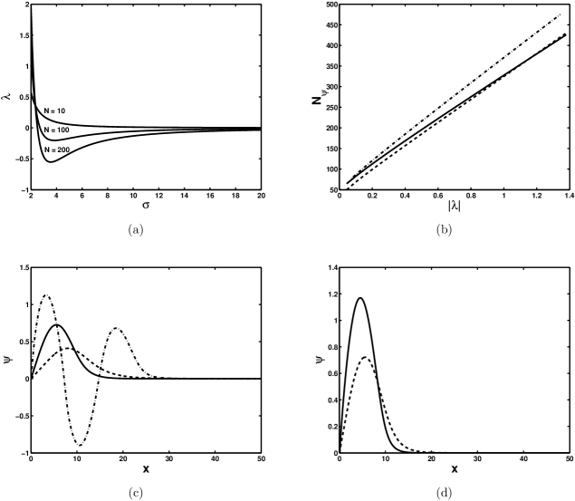
Figure 1: The analysis of solutions of Eq. (II.2) in 2D case. (a) The function $\lambda(\sigma)$ obtained on the basis of Eq. (II.2) using a “guess” function $\psi=\psi_{g}$ (25) for different values of $N_{0}$. (b) The dependence $N_{\psi}(\lambda)$: solid line corresponds to a numerical solution of Eq. (II.2), dashed line represents an “analytical” curve corresponding to minimal $\lambda_{a}$, and dash-dotted line corresponds to a numerical solution of Eq. (II.2) at the absence of the term $(d-1)/x\times\psi\partial|\psi|^{2}/\partial x$ (see Ref. DavYakZal05 ). (c) Examples of solutions of Eq. (II.2) obtained for $N_{0}=100$; solid line: $N_{\psi}\approx 113$, $\lambda\approx-0.20$, and $\sigma\approx 3.83$ (optimal parameters minimizing $\lambda$), dashed line: $N_{\psi}\approx 70$, $\lambda\approx-0.06$, and $\sigma\approx 9.56$, and dash-dotted line: $N_{\psi}\approx 595$, $\lambda\approx-0.06$, and $\sigma\approx 2.83$. (d) The same as in panel (c) for $N_{0}=200$; solid line: $N_{\psi}\approx 210$, $\lambda\approx-0.55$, and $\sigma\approx 3.55$ (optimal parameters), dashed line: $N_{\psi}\approx 113$, $\lambda\approx-0.20$, and $\sigma\approx 7.91$, and dash-dotted: $N_{\psi}\approx 113$, $\lambda\approx-0.20$, and $\sigma\approx 2.64$. Note that in the latter case dashed and dash-dotted lines practically coincide.

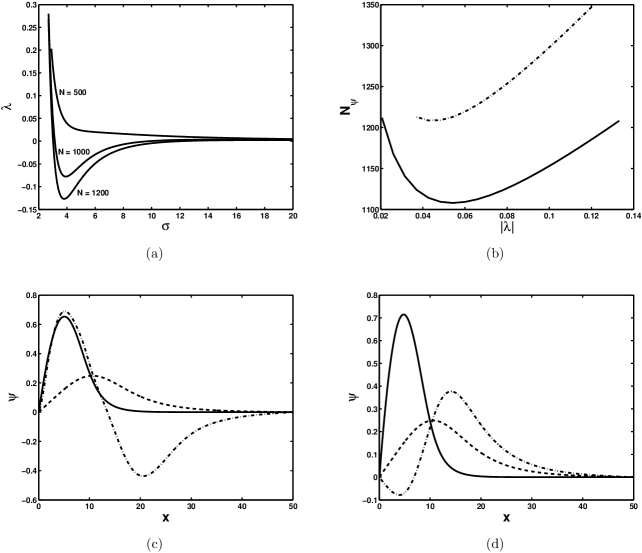
Figure 2: Panels (a) and (b) are the same as in Fig. 1(a,b) but correspond to 3D case. (c) Examples of stable solutions of Eq. (II.2) [right-handed branch in panel (b)] obtained for $N_{0}=1100$; solid line: $N_{\psi}\approx 1150$, $\lambda\approx-0.10$, and $\sigma\approx 3.90$ (optimal parameters), dashed line: $N_{\psi}\approx 1429$, $\lambda\approx-0.01$, and $\sigma\approx 8.22$, and dash-dotted line: $N_{\psi}\approx 1219$, $\lambda\approx-0.01$, and $\sigma\approx 3.10$. (d) The same as in panel (c) for $N_{0}=1200$; solid line: $N_{\psi}\approx 1197$, $\lambda\approx-0.13$, and $\sigma\approx 3.80$ (optimal parameters), dashed line: $N_{\psi}\approx 1429$, $\lambda\approx-0.01$, and $\sigma\approx 8.82$, and dash-dotted line: $N_{\psi}\approx 4354$, $\lambda\approx-0.01$, and $\sigma\approx 3.04$.

One can see that the function $\lambda(\sigma)$ has a minimum if $N_{0}>N_{\mathrm{cr}}$. In two dimensional case the critical number of plasmons can be easily found: $N_{\mathrm{cr}}=8\pi$. Note that one can expect the stability of a soliton with respect to the collapse if $\lambda<0$ for $d=2$, whereas in 3D case there is some range of positive $\lambda$ which corresponds to uncollapsing solutions.

The solutions which correspond to various values of $\lambda$, $\sigma$, and $N_{\psi}$ are shown in Fig. 1(c,d), for $d=2$, and in Fig. 2(c,d), for $d=3$. A “guess” function which does not correspond to the minimum of the function $\lambda(\sigma)$ also gives some solitonic solution of Eq. (II.2), however the convergence is much worse than in the minimal $\lambda$ case. Indeed, $N_{\psi}$ significantly differs from $N_{0}$ for such a solution. When the deviation from the minimal $\lambda$ is big, although $\lambda$ remains to be negative, no regular solutions can be found and the system capsizes into chaos. Thus these “nonoptimal” solutions seem to be unstable.

To analyze the stability of the found solutions we present the $N_{\psi}(\lambda)$ dependence in Fig. 1(b), for $d=2$, and in Fig. 2(b), for $d=3$. Note these curves were built for “guess” functions corresponding to a minimal $\lambda$. Applying the Vakhitov–Kolokolov criterion SulSul99p72 to the results shown on these plots one can conclude that the presented solutions are stable in 2D case, whereas some unstable solitons can exist in three dimensions. For $d=3$, a stable solution can be generated starting from a threshold plasmon number $N_{\mathrm{cr}}\approx 1100$ and at $|\lambda|>0.05$ (see also the discussion in Sec. IV). We show an example of a unstable soliton in Fig. 3.

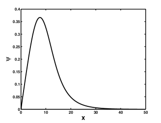
Figure 3: An example of the unstable solution of Eq. (II.2) [left-handed branch in Fig. 2(b)] obtained for $N_{0}=770$. It corresponds to $N_{\psi}\approx 1174$, $\lambda\approx-0.02$, and $\sigma\approx 4.20$.

In Fig. 1(b), for $d=2$, one can see that the new term in Eq. (II.2), $\sim(d-1)/x\times\psi\partial|\psi|^{2}/\partial x$, does not produce any significant effect (compare solid and dash-dotted lines). In 3D case, Fig. 2(b), the difference is just quantitative: the critical plasmon number and critical frequency are shifted. Therefore our results are in agreement with Ref. DavYakZal05 where NLSE with a nonlocal term was analyzed. One should also notice that the numerical curve in Fig. 1(b) (solid line) is in a good agreement with the “analytical” $\lambda(N_{\psi})$ dependence (dashed line), $\lambda_{a}=-(N_{\psi}-8\pi)^{2}/(88\pi N_{\psi})$, found from Eq. (II.2) with help of the “guess” function (25).

IV Applications

Stable spatial solitons, involving nonlocal nonlinearities, similar to plasma structures described in the present work, were reported to be obtained in various laboratory experiments in plasma physics, condescended matter, and nonlinear optics (see, e.g., reviews Kro04 ; Sku06 ; ShuEli10 and references therein). Another opportunity for the physical realization of plasmoids described in Secs. II and III consists in their implementation as a rare natural atmospheric electricity phenomenon called a ball lightning (BL) Ste99 .

According to the BL observations, most frequently it has a form of a rather regular sphere with the diameter of $(20-50)\thinspace\text{cm}$ Ste99p11 . However big BLs with the size more than one meter were reported to exist BycGolNik10 . Besides spherical BL, snake-like objects were observed BycGolNik10 . The lifetime of BL can be up to several minutes Ste99p11 . The estimates of energy of BL were obtained only in cases when it produced some destruction while disappearing. These estimates give for the energy of BL the value in the range (several kJ – several MJ) BycGolNik10p214 . However, since in many cases BL disappears just fading, one should assume that a very low energy BL can exist.

Numerous BL models are reviewed in Ref. theoryBL . Despite very exotic theoretical descriptions of BL were proposed, it is most probable that this object is a plasma based phenomenon. In Refs. DvoDvo ; Dvo10 we developed a BL model based on radial oscillations of electron gas in plasma, studying these oscillations in both classical and quantum approaches. The present work is a development of our BL model. As in our previous studies, here we also treat BL on the basis of radial oscillations of electrons. However, as we show in Secs. II and III, local and nonlocal electron nonlinearities as well as the interaction of electrons with ions play an important role for the stability of an axially or spherically symmetric plasmoid. For example, the inhomogeneity of ion density was not accounted for in Ref. DvoDvo . It should be noted that the idea that spherically symmetric oscillations of electrons underlie the BL phenomenon was independently put forward in Ref. Shm03 .

In Fig. 4 we present the characteristics of axially symmetric (snake-like BL BycGolNik10 ) and spherically symmetric (spherical BL) plasmoids calculated on the basis of the results of Sec. III.

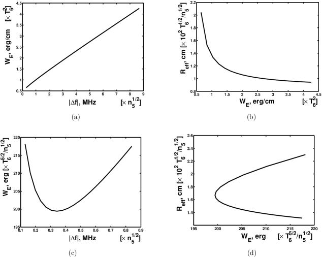
Figure 4: Physical characteristics of axial [panels (a) and (b)] and spherical [panels (c) and (d)] plasmoids expressed in terms of $T_{6}=T_{e}/10^{6}\thinspace\text{K}$ and $n_{5}=n_{0}/10^{5}\thinspace\text{cm}^{-3}$. (a) The energy density of electric field vs. the frequency shift. (b) The effective radius vs. the energy density. (c) The total energy of electric field vs. the frequency shift. Stable plasmoids correspond to the right-handed branch. (d) The effective radius vs. the total energy. Stable plasmoids correspond to the lower branch.

The total energy of electric field inside a plasmoid (energy density in 2D case) and the effective plasmoid radius are defined as

$$W_{\mathrm{E}}=\frac{1}{8\pi}\int E^{2}\mathrm{d}V,\quad R_{\mathrm{eff}}^{2}=\frac{1}{8\pi W_{\mathrm{E}}}\int r^{2}E^{2}\mathrm{d}V.$$ (26)

The frequency of the total oscillation, including the main harmonic oscillation which was separated in the derivation of Eq. (II.2), is $f=f_{p}-|\Delta f|$, where $f_{p}=2.8\times\sqrt{n_{5}}\thinspace\text{MHz}$ is the Langmuir frequency. Here we take into account that frequency shift $\Delta f$ for a stable plasmoid is negative [see Figs. 1(a) and 2(a)].

One can see in Fig. 4 that in frames of our BL model we predict the existence of low energy ($W_{\mathrm{E}}\gtrsim\text{erg/cm}$ in 2D case and $W_{\mathrm{E}}\gtrsim 10^{2}\thinspace\text{erg}$ in 3D case) plasma structures with the typical size $R_{\mathrm{eff}}\lesssim 1.5\thinspace\text{m}$. This kind of plasmoids should appear in low density $n_{e}\sim 10^{5}\thinspace\text{cm}^{-3}$ and hot $T_{e}\sim 10^{6}\thinspace\text{K}$ plasma. Such a density of plasma can well exist in the Earth ionosphere Per97 . A linear lightning can provide the plasma heating up to $T_{e}\sim 10^{6}\thinspace\text{K}$ since, e.g., $T_{i}\sim 10^{4}\thinspace\text{K}$ in the lightning channel RakUma06 . Thus we can assume that such high temperatures of plasma can be present in some localized area of ionosphere during a thunderstorm, making possible the existence of plasma structures described in the present work. It is interesting to notice that several meters objects were reported to appear in the BL observations near airplanes airplane .

To demonstrate the stability of the described plasmoids with respect to decay, in Fig. 5 we present the ratio $W_{\mathrm{E}}/W_{k}$ versus $W_{\mathrm{E}}$, where $W_{k}=(3/2)n_{0}T_{e}V_{\mathrm{eff}}$ is the total thermal energy of a plasmoid (energy density in 2D case) and $V_{\mathrm{eff}}$ is the effective volume of a plasmoid, which is equal to $\pi R_{\mathrm{eff}}^{2}$ for $d=2$ and to $(4/3)\pi R_{\mathrm{eff}}^{3}$ for $d=3$.

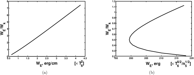
Figure 5: The ratio $W_{\mathrm{E}}/W_{k}$ vs. $W_{\mathrm{E}}$ for (a) 2D plasmoid and (b) 3D plasmoid. In the panel (b) a stable plasmoid corresponds to the upper branch and an unstable one to the lower branch.

Indeed, hot electrons with $T_{e}\sim 10^{6}\thinspace\text{K}$ could just escape the plasmoid volume making it unstable. One can however see in Fig. 5 that for stable plasma structures the ratio $W_{\mathrm{E}}/W_{k}$ has a tendency to increase reaching the unit value at a certain soliton energy ($W_{\mathrm{E}}\approx 1\thinspace\text{erg/cm}$ for $d=2$ and $W_{\mathrm{E}}\approx 215\thinspace\text{erg}$ for $d=3$). It means that hot electrons will not escape form the plasmoid volume as soon its energy has this critical value. It should be noticed that an unstable plasmoid, corresponding to the lower branch in Fig. 5(b), will lose electrons since $W_{\mathrm{E}}/W_{k}<1$ always.

Comparing the predicted plasmoid properties with the characteristics of circumterrestrial (not ionospheric) BL one can say that our model is not directly applicable for the description of such an object since its energy $\gtrsim 10\thinspace\text{kJ}$ and the size $\sim(20-50)\thinspace\text{cm}$ are beyond our predictions. We can however use our model at the initial stages of the plasmoid formation when the amplitude of the electric field is so high since in Eq. (II.2) we keep only cubic nonlinearity. Higher nonlinear terms, which seem to be important for denser plasma, can explain smaller size and bigger energy content.

A natural plasmoid appearing in circumterrestrial atmosphere is surrounded by the neutral gas. It means that plasma in the interior of a plasmoid should be maintained in the state with proper ionization during its lifetime. It is however known Smi93 that plasma of a low energy plasmoid, without an internal energy source, will lose energy and recombine back to a neutral gas in the millisecond time scale at the atmospheric pressure. Thus the lifetime of such an object will be extremely short. It was suggested that under certain conditions plasma can reveal superconducting properties supercond . This mechanism could prevent the energy losses and thus the recombination, providing the long lifetime of a low energy plasmoid.

V Conclusion

In conclusion we mention that in the present work we have studied axially and spherically symmetric Langmiur solitons in warm plasma. In Sec. II we started with the discussion of radially symmetric oscillations of electrons in plasma and then separated the motions on different time scales. In Sec. II.1 we briefly reviewed the previous works on the theory of stable plasma structures which involved local electron nonlinearities. Then, in Sec. II.2 we have calculated the contribution of the slowly varying electron density to the electron pressure and derived, together with the results of Ref. DavYakZal05 , the new NLSE (II.2) which accounts for nonlocal electron nonlineariries. These additional nonlinear terms do not disappear in one dimensional case. This fact was also demonstrated in Appendix A using Lagrange variables.

The solutions of this new NLSE, rewritten in the equivalent form (II.2) for the radially symmetric case, have been analyzed numerically in Sec. III. We presented the examples of some of the solutions of Eq. (II.2) [see Fig. 1(c,d) and Fig. 2(c,d)] and analyzed their stability. It has been found that solutions in 2D case are stable, whereas in tree dimensions some unstable solitons can exist. We also compared out results with Ref. DavYakZal05 , where analogous NLSE was considered.

In Sec. IV we suggested that the described axially and spherically symmetric solitons can be realized in the form of a natural plasmoid, a ball lightning. We have computed the characteristics of such a plasma structure, like energy and radius (see Fig. 4), predicted in frames of our model. Comparing these characteristics with the properties of a natural plasmoid one concludes that our model describes a low energy BL which can exist in hot ionospheric plasma. Note that in many cases BLs were observed form airplanes airplane at high altitudes. We also examined the stability of plasmoids with respect to decay because of the escape of hot electrons.

We have already considered a BL model based on radial oscillations of electrons in our previous publications DvoDvo ; Dvo10 . In the present work we performed more detailed analysis of electron nonlinearities and showed that they play a crucial role for the stability of a plasmoid. Although plasma structures described in the present work does not reproduce all the properties of circumterrestrial (not ionospheric) BL Ste99p11 ; BycGolNik10p214 , we can use our results for the description of the BL formation, when the amplitude of the electric field is not so big.

As we have found in Sec. III [see also Fig. 4(a,c)], the total frequency of electron oscillations is less than Langmuir frequency, since the frequency shift $\Delta f$ is negative. It is important fact for the future experimental studies of BL. For example, the electron density in a linear lightning discharge can be $\sim 10^{17}\thinspace\text{cm}^{-3}$ RakUma06p163 , giving for the plasma frequency a huge value of $\sim 10^{3}\thinspace\text{GHz}$. In a laboratory it is extremely difficult to create a strong electromagnetic field of such a frequency to generate BL. However, if the frequency of electron oscillations has a tendency to decrease, it can facilitate the plasmoid generation.

Appendix A Lagrange variables

The propagation of waves in plasma was analyzed in Sec. II.1 using Euler variables which are more convenient for the practical purposes. There is, however, a Lagrange approach for the treatment of plasma waves. Instead of describing of plasma characteristics, like velocity, density etc, in a certain point of space, one can study the dependence of these quantities on the initial coordinates of plasma particles.

Let us change the variables $(r,t)\to(\rho,\tau)$ in Eqs. (1) and (5) as

$$r= \rho+\xi(\rho,\tau),\quad t=\tau,$$

$$\frac{\partial}{\partial\rho}= \frac{\partial r}{\partial\rho}\frac{\partial}{\partial r},\quad\frac{\partial}{\partial\tau}=\frac{\partial}{\partial t}+v_{e}\frac{\partial}{\partial r},$$ (27)

where $\rho$ is the initial coordinate of an electron, $\xi$ is deviation of an electron from the equilibrium, and $\tau$ is the new temporal variable. An electron is supposed to be in the equilibrium initially, $\xi(\rho,0)=0$. In Eq. (A) we use the definition of electron velocity, $\partial r/\partial\tau=\partial\xi/\partial\tau=v_{e}$. Unlike the Euler picture, the continuity equation in Lagrange variables can be integrated and it does not contain the time derivative,

$$n_{0}\rho^{d-1}=n_{e}r^{d-1}\frac{\partial r}{\partial\rho}$$ (28)

where $n_{0}=n_{e}(\tau=0)$ is the initial (unperturbed) electron density, which is supposed to be uniform.

Using Eqs. (A) and (28) we can obtain from Eq. (1) a single nonlinear equation for electron velocity,

$$\ddot{v}_{e} +\omega_{p}^{2}\frac{n_{i}}{n_{0}}v_{e}+v_{e}\dot{v}_{e}\frac{d-1}{r}$$

$$+3v_{\mathrm{T}}^{2}\bigg{[}\frac{2r^{\prime\prime}v_{e}^{\prime}}{r^{\prime 3}}-\frac{v_{e}^{\prime\prime}}{r^{\prime 2}}+(d-1)\left(\frac{v_{e}}{r^{2}}-\frac{v_{e}^{\prime}}{\rho r^{\prime 2}}-\frac{v_{e}r^{\prime\prime}}{rr^{\prime 2}}\right)$$

$$+(d-1)^{2}\frac{v_{e}}{r}\left(\frac{1}{\rho r^{\prime}}-\frac{1}{r}\right)\bigg{]}=0,$$ (29)

where a “dot” and a “prime” mean the derivatives with respect to $\tau$ and $\rho$. To derive Eq. (A) we assume that electrons obey the adiabatic equation $p/n_{e}^{\gamma_{e}}=\text{const}$, where $p$ is electron pressure [$p_{ij}=p\delta_{ij}$, see Eq. (2)] and $\gamma_{e}=3$ since we study electrostatic oscillations Jac65 . Analogous assumptions were taken in Ref. InfRow87 to study the nonlinear one-dimensional plasma waves in warm plasma within the Lagrange picture.

Note that Eq. (A) is an exact one, which does not suppose any expansion over a small parameter. We can, however, discuss the small deviations from the equilibrium position,

$$\ddot{v}_{e} +\omega_{p}^{2}\left(1+\frac{n}{n_{0}}\right)v_{e}-3v_{\mathrm{T}}^{2}\frac{\partial}{\partial\rho}\left[\frac{1}{\rho^{d-1}}\frac{\partial}{\partial\rho}\left(\rho^{d-1}v_{e}\right)\right]$$

$$+v_{e}\dot{v}_{e}\frac{d-1}{\rho}+3v_{\mathrm{T}}^{2}\bigg{[}2(\xi^{\prime\prime}v_{e}^{\prime}+v_{e}^{\prime\prime}\xi^{\prime})$$

$$+(d-1)(d-3)\frac{v_{e}\xi}{\rho^{3}}+(d-1)\left(2\frac{v_{e}^{\prime}\xi^{\prime}}{\rho}-\frac{v_{e}\xi^{\prime\prime}}{\rho}\right)$$

$$-(d-1)^{2}\frac{v_{e}\xi^{\prime}}{\rho^{2}}\bigg{]}=0,$$ (30)

keeping only quadratic nonlinearities. As in Sec. II.1, $n=n_{i}-n_{0}$, stays for the perturbation of the ion density in Eq. (A).

It can be noticed that Eq. (A) has analogous structure as Eq. (II.2) before the separation of the main harmonic (for the details see, e.g., Ref. MusRubZak95 ). We can see, however, that nonlinear terms do not disappear completely at $d=1$ if we consider warm plasma with $T_{e}\neq 0$. One can also notice that these nonvanishing nonlinear terms arise from the pressure term in the initial plasma hydrodynamics equations (1). Analogous conclusion was obtained in Sec. II.2 using Euler coordinates. Note that the nonlinear plasma waves were also studied in Refs. InfRow87 ; Daw59 . It was found in Ref. InfRow87 that the nonlinear terms are important even for one dimensional plasma oscillations for the case of nonzero electron temperature, which is in agreement with our results [see Eqs. (II.2) and (A)].

References

- (1) E. Infeld and G. Rowlands, Nonlinear waves, solitons and chaos, (Cambridge, Cambridge Univ. Press, 1990).
- (2) W. Królikowski, et al., J. Opt. B: Quantum Semiclass. Opt. 6, S288 (2004), nlin/0402040; C. Rotschild, et al., Nature Phys. 2, 769 (2006).
- (3) S. Skupin, et al., Phys. Rev. E 73, 066603 (2006), nlin/0603014.
- (4) P. K. Shukla and B. Eliasson, Phys. Uspekhi 53, 51 (2010), 0906.4051 [physics.plasm-ph]
- (5) V. E. Zakharov, Sov. Phys. JETP 35, 908 (1972).
- (6) M. V. Goldman, Rev. Mod. Phys. 56, 709 (1984).
- (7) E. A. Kuznetsov, Sov. J. Plasma Phys. 2, 178 (1976); V. L. Malkin, Sov. Phys. JETP 63, 34 (1986).
- (8) M. M. Škorić and D. ter Haar, Physica C 98, 211 (1980).
- (9) C. Sulem and P.-L. Sulem, The nonlinear Schrödinger equation: self-focusing and wave collapse, (NY, Springer, 1999), pp. 245–262.
- (10) A. G. Litvak, et al., Sov. J. Plasma Phys. 1, 31 (1975).
- (11) T. A. Davydova, A. I. Yakimenko, and Yu. A. Zaliznyak, Phys. Lett. A 336, 46 (2005), physics/0408023.
- (12) P. Y. Cheung and A. Y. Wong, Phys. Fluids 28, 1538 (1985).
- (13) E. Infeld and G. Rowlands, Phys. Rev. Lett. 58, 2063 (1987).
- (14) F. Chen, Introduction to plasma physics, (Moscow, Mir, 1987), pp. 292–295 and 388.
- (15) F. Haas and P. K. Shukla, Phys. Rev. E 79, 066402 (2009), 0902.3584 [physics.plasm-ph]; G. Simpson, C. Sulem, and P. L. Sulem, Phys. Rev. E 80, 056405 (2009), 0910.1810 [math.AP].
- (16) D. Anderson, Phys. Rev. A 27, 3135 (1983).
- (17) See pp. 72–75 in Ref. SulSul99 .
- (18) M. Stenhoff, Ball lightning: an unsolved problem in atmospheric physics, (NY, Kluwer, 1999).
- (19) See pp. 11–21 in Ref. Ste99 .
- (20) V. L. Bychkov, A. I. Nikitin, and G. C. Dijkhius, in The atmosphere and ionosphere: dynamics, processing and monitoring, ed. by V. L. Bychkov, G. V. Golubkov, and A. I. Nikitin, (Heidelberg, Springer, 2010), p. 204.
- (21) See pp. 214–216 in Ref. BycGolNik10 .
- (22) See pp. 197–238 in Ref. Ste99 and pp. 270–295 in Ref. BycGolNik10 .
- (23) M. Dvornikov and S. Dvornikov, in Advances in plasma physics research, vol. 5, ed. by F. Gerard (NY, Nova Science, 2007), pp. 197–212, physics/0306157; M. Dvornikov, S. Dvornikov, and G. Smirnov, Appl. Math. Eng. Phys. 1, 9 (2001), physics/0203044.
- (24) M. Dvornikov, Phys. Scr. 81, 055502 (2010), 1002.0764 [physics.plasm-ph]; ibid. 83, 017004 (2011), 1101.1986 [physics.plasm-ph]
- (25) M. L. Shmatov, J. Plasma Phys. 69, 507 (2003).
- (26) A. L. Peratt, Astrophys. Space Sci. 242, 93 (1997).
- (27) V. A. Rakov and M. A. Uman, Ligntning: physics and effects, (Cambridge, Cambridge Univ. Press, 2006), p. 7.
- (28) See pp. 109–122 in Ref. Ste99 .
- (29) B. M. Smirnov, Phys. Rep. 224, 151 (1993).
- (30) G. C. Dijkhuis, Nature 284, 150 (1980); M. I. Zelikin, J. Math. Sci. 151, 3473 (2008); see also B. E. Meierovich Phys. Scr. 29, 494 (1984).
- (31) See p. 163 in Ref. RakUma06 .
- (32) J. D. Jackson, Classical electrodynamics, (Moscow, Mir, 1965), pp. 369–374.
- (33) S. L. Musher, A. M. Rubenchik, and V. E. Zakharov, Phys. Rep. 252, 177 (1995).
- (34) J. M. Dawson, Phys. Rev. 113, 383 (1959).