Conicoid Mirrors

Abstract

The first order equation relating object and image location for a mirror of arbitrary conic-sectional shape is derived. It is also shown that the parabolic reflecting surface is the only one free of aberration and only in the limiting case of distant sources.

LABEL:FirstPage1 LABEL:LastPage#1

I
Introduction

Most elementary treatments of reflecting surfaces restrict their attention to the spherical case. In this standard case, and assuming the paraxial approximation (all angles are small and all rays are close to the optical axis), the resulting equation relating the axial object and image positions and the radius of curvature of the reflecting spherical surface is

$$\frac{1}{v}+\frac{1}{u}=\frac{2}{r},$$ (1)

where all parameters are one dimensional coordinates which locate the image ($v$), object ($u$), and center of curvature ($r$) with respect to the vertex (the intersection of the surface with the optical axis) pedrotti . A convention is typically assumed in which light rays travel from left to right in all figures. The origin of the one dimensional coordinate system employed coincides with the vertex, and locations to the right (left) of the vertex are positive (negative).

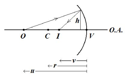
Figure 1: The spherical reflecting surface.

The paraxial approximation is equivalent to a first order approximation in the height ($h$) of the incidence point (on the surface) of a reflecting ray. To higher order, it is found that

$$v=v(u,r,h).$$ (2)

Consequently, spherical mirrors are aberrant at higher order since the image location is not independent of the height, $h$.

This paper represents a more general treatment of a mirror than is typically found in the literature. The reflecting surface is assumed to be a conicoid, the surface of revolution generated by a conic. Equation (1) is then derived as the special case of a spherical surface and to first order in $h$. Special cases are analyzed as a function of asphericity, or departure from the spherical, of the reflecting surface. The parabolic surface is shown to be uniquely special in that

$$\frac{dv}{dh}=0$$ (3)

to all orders for objects at infinity ($u\rightarrow-\infty$).

II Analysis: Conicoid Case

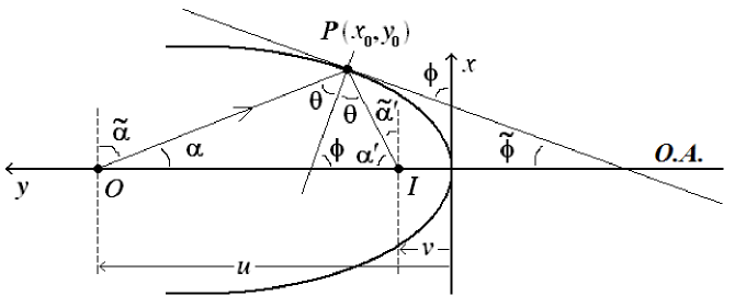
Figure 2: Conicoid mirror.

In Fig. 2, a conicoid reflecting surface is depicted with equation

$$x^{2}=\frac{1}{a}y-\sigma y^{2},\;a=-\frac{1}{2r}>0,$$ (4)

where $r$ is the radius of curvature of the surface at the vertex, and $\sigma=1-e^{2}$ is the shape factor and is related to the standard eccentricity (see Appendix I or, for example, conicoid ). For a sphere, $\sigma=1$, whereas for a paraboloid $\sigma=0$. Note that the $xy$ coordinate system is set on its side so that $+\hat{y}$ coincides with the negative direction on the optical axis (O.A.) as defined in Fig. 1 of the Introduction. Consequently, the radius of curvature, $r$, at the origin for any concave conicoid (i.e., opening to the left) will be considered negative. In Fig. 2, a representative case is depicted with $u<0$, the location of the object, and $v<0$, the location of the image. The figure displays an incident ray, $\overline{OP}$, emanating from the object at $O$ and a reflected ray, $\overline{IP}$, passing through the image at $I$. From the figure, the line $\overline{OP}$ has equation in the $xy$-plane

$$y-(-u)=x\tan\left(-\tilde{\alpha}\right)=-\frac{x}{\tan\alpha}.$$ (5)

Similarly, the line $\overline{IP}$ has equation

$$y-(-v)=x\tan\tilde{\alpha}^{\prime}=\frac{x}{\tan\alpha^{\prime}}.$$ (6)

Consequently,

$$\tan\alpha =-\frac{x_{0}}{y_{0}+u},$$ (7)

$$\tan\alpha^{\prime} =\frac{x_{0}}{y_{0}+v},$$ (8)

where $(x_{0},y_{0})$ is the point of reflection, $P$, on the surface. From the figure, it follows that

$$\phi=\alpha+\theta,$$ (9)

where

$$\tan\phi=\left.\frac{dy}{dx}\right|_{P}=\frac{2ax_{0}}{1-2\sigma ay_{0}},$$ (10)

and

$$\alpha^{\prime}+\theta+\phi=\pi.$$ (11)

Therefore

$$\tan\left(\alpha-\alpha^{\prime}\right) =\tan\left(2\phi-\pi\right)$$ (12)

$$\frac{\tan\alpha-\tan\alpha^{\prime}}{1+\tan\alpha\tan\alpha^{\prime}} =\frac{2\tan\phi}{1-\tan^{2}\phi}.$$ (13)

Substituting for the tangents from above yields

$$\left(\frac{1}{v}+\frac{1}{u}\right)\left[1-\frac{4\sigma a^{2}y_{0}^{2}}{\left(1-2\sigma ay_{0}\right)^{2}}\right]-\left(\frac{1}{uv}\right)\frac{2y_{0}\left[1+2\left(1-\sigma\right)ay_{0}\right]}{\left(1-2\sigma ay_{0}\right)^{2}}=-\frac{4a}{1-2\sigma ay_{0}}$$ (14)

$$\left(\frac{1}{v}+\frac{1}{u}\right)\left[1-4\sigma ay_{0}-4\sigma\left(1-\sigma\right)a^{2}y_{0}^{2}\right]-\left(\frac{1}{uv}\right) 2y_{0}\left[1+2\left(1-\sigma\right)ay_{0}\right]\hskip 32.52127pt$$

$$\hskip 43.36243pt=-4a\left(1-2\sigma ay_{0}\right).$$ (15)

Now let $h\equiv x_{0}$ be the height of the incidence point $P$ for a particular ray from the source object at $O$, then in the paraxial approximation ($h\ll 1$),

$$y_{0}=ah^{2}+\sigma a^{3}h^{4}+\mathcal{O}(h^{6}).$$ (16)

Equation (15) can then be rewritten to fourth order as

$$\left(\frac{1}{v}+\frac{1}{u}-\frac{2}{r}\right) =\left[2a\left(\frac{1}{uv}\right)-8\sigma a^{3}\right]h^{2}$$

$$\hskip 36.135pt+\left[4\sigma a^{4}\left(\frac{1}{v}+\frac{1}{u}\right)+2\left(3\sigma+2\right)a^{3}\left(\frac{1}{uv}\right)-24\sigma^{2}a^{5}\right]h^{4}.$$ (17)

Note that there is aberration in imaging a finite axial point since there is no confluence in the rays from $O$. Also note that there is no fixed shape factor $\sigma$ that eliminates aberration to second order and higher. To first order, all conicoids obey the same relation

$$\frac{1}{v}+\frac{1}{u}=\frac{1}{f}+\mathcal{O}(h^{2}),$$ (18)

which coincides, of course, with the Gaussian (first order approximation) equation for a spherical mirror with focal length $f=r/2$.

From Eq. (15) it follows that for objects at infinity ($u\rightarrow-\infty$) and a parabolic shape ($\sigma=0$), the image forms at $v=f$ regardless of the height of the incidence ray, therefore, there is no aberration for such imaging.

III Analysis: General Case

It is desirable to know to what extend the results of the previous section are pathological to conicoids. With this in mind consider the most general axi-symmetric surface of revolution (about the y-axis) as a reflector

$$y=\sum_{n=1}^{\infty}c_{2n}x^{2n}.$$ (19)

Equation (13) is easily generalized to

$$\frac{\tan\alpha-\tan\alpha^{\prime}}{1+\tan\alpha\tan\alpha^{\prime}}=\frac{2y^{\prime}}{1-y^{\prime 2}},$$ (20)

where $y^{\prime}=\left.\frac{dy}{dx}\right|_{P}$. In general, for a given axial object location, the image location (or intersection point of the reflected ray with the optical axis) is a function of the object location and the reflection point

$$v=v(u,x_{0})\text{ with }y_{0}=y(x_{0}).$$ (21)

A reflecting surface is free of aberration if

$$v^{\prime}\equiv\frac{dv}{dx_{0}}=0\;\forall u.$$ (22)

Equation (20) can be implicitly differentiated to yield

$$\frac{v^{\prime}}{v}\left\{2y^{\prime}+\frac{x-xy^{\prime 2}+2yy^{\prime}}{u}\right\} =\left(\frac{1}{v}+\frac{1}{u}\right)\left\{\frac{\left(1+y^{\prime 2}\right)\left(xy^{\prime\prime}-y^{\prime}\right)}{y^{\prime}}\right\}_{1}$$

$$\;\;\;\;+2\left(\frac{1}{uv}\right)\left\{\frac{\left(1+y^{\prime 2}\right)\left[\left(xy^{\prime\prime}-y^{\prime}\right)y+xy^{\prime 2}\right]}{y^{\prime}}\right\}_{2}.$$ (23)

The aberration-free surface must satisfy $\left\{\cdots\right\}_{1}=\left\{\cdots\right\}_{2}=0$. However, it is evident from Eq. (23) that this cannot be obtained trivially. For the special case in which the object is at infinity though, the aberration-free surface must only satisfy $\left\{\cdots\right\}_{1}=0$, and this leads to a defining equation for the surface

$$xy^{\prime\prime}-y^{\prime}=0.$$ (24)

This is a linear differential equation whose general solution can most easily be found by the reduction in order method to give the general solution $y=Ax^{2}+B$. This further reduces to the particular solution of Eq. (38), found by another method, after the two needed boundary conditions are invoked.

IV Conclusion

Most elementary treatments of mirrors lack a discussion of the first order equation relating object and image locations in the case of arbitrary mirror shape. The default reflecting surface is always the spherical one. In fact, a simple analysis yields that all axi-symmetric, conic, reflecting surfaces of revolution (conicoids) in the first order, paraxial approximation satisfy the same (Gaussian) equation

$$\frac{1}{v}+\frac{1}{u}=\frac{2}{r},$$ (25)

where $r$ is the radius of curvature of the surface at its vertex.

Aberrations enter at second order and cannot be eliminated for finite object locations by any fixed shape. However, for objects at infinity, or specifically, for incoming light parallel to the optical axis, there is a unique reflecting shape that is free of aberration – the parabolic one.

Appendix A Derivation of the Conic Section Equation

Starting with the general form of a conic section in Cartesian coordinates,

$$Ax^{2}+Bxy+Cy^{2}+Dx+Ey+F=0,$$ (26)

assume $x$-reflection symmetry, so that the equation reduces to

$$x^{2}+C^{\prime}y^{2}+E^{\prime}y+F^{\prime}=0.$$ (27)

Next the curve is shifted so the vertex coincides with the origin, $y\rightarrow y+k,$ with $2C^{\prime}k+E^{\prime}=\pm\sqrt{E^{\prime 2}-4C^{\prime}F^{\prime}}$. If the form is further constrained so that the curve lies in $y\geq 0$ half-plane, then the positive root is required, and this yields

$$x^{2}=\sqrt{E^{\prime 2}-4C^{\prime}F^{\prime}}y-C^{\prime}y^{2},$$ (28)

or in terms of new parameters

$$x^{2}=\frac{1}{a}y-\sigma y^{2},$$ (29)

where $a>0$. The signed curvature of this curve at the origin is

$$k\equiv\left.\frac{y^{\prime\prime}}{\left(1+y^{\prime 2}\right)^{3/2}}\right|_{(0,0)}=2a>0.$$ (30)

Given the optics conventions adopted here as described in the Introduction and depicted in Figures 1 and 2, the radius, $r$, of the osculating circle at the origin for a concave conicoid is considered negative. The radius of curvature is therefore related to the parameter $a$

$$k=2a=-\frac{1}{r}>0,$$ (31)

and

$$\frac{1}{a}=-2r.$$ (32)

From Eq. (29) it follows that $\sigma=0$ corresponds to a parabola. By putting Eq. (29) into canonical form

$$\frac{x^{2}}{\left(\frac{1}{4\sigma a^{2}}\right)}+\frac{\left(y-\frac{1}{2\sigma a}\right)^{2}}{\left(\frac{1}{4a^{2}}\right)}=1,$$ (33)

it becomes clear that $\sigma=1$ corresponds to a circle with radius $\left|r\right|=\frac{1}{2a}$. The equation describes a hyperbola when $\sigma<0$. For $0<\sigma<1$, the equation describes an oblate ellipse (with respect to the y-axis), and it describes a prolate ellipse for $\sigma>1$. In fact, from Eq. (33), the shape factor, $\sigma$, can be related to the standard eccentricity

$$\sigma=1-e^{2}.$$ (34)

Appendix B Alternate Derivation of the Paraboloid in the Limiting Object Distance Case

An alternate solution (to that of Section III) is presented for the exact conicoid shape in the limit that the object distance approaches infinity ($u\rightarrow\infty$). Applying the law of reflection (based on Fermat’s principle of stationary optical path) to a parallel (to the optical axis) ray (from a distant object) incident on an unknown conicoid surface, results in the optical path displayed in Fig. 3.

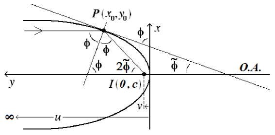
Figure 3: Paraxial incident ray on unknown conicoidal surface.

Applying Eq. (8) to the present special case, it follows that

$$\tan 2\tilde{\phi}=\frac{2\tan\tilde{\phi}}{1-\tan^{2}\phi}=\frac{x_{0}}{y_{0}-c}.$$ (35)

If the notation is changed and the $y$ variable is shifted for convenience, $(x_{0},y_{0})\rightarrow(x,y+c),\;\tan\tilde{\phi}=\frac{dx}{dy}$, then Eq. (35) can be reduced to either a homogeneous nonlinear ordinary differential equation (ODE) of the form

$$\frac{dx}{dy}=\frac{-y+k\sqrt{x^{2}+y^{2}}}{x},\;k=1,\;x(-c)=0$$ (36)

or to a nonlinear Clairaut ODE clairaut of the form

$$w=y\frac{dw}{dy}+\frac{1}{4}\left(\frac{dw}{dy}\right)^{2},\;w=x^{2}.$$ (37)

Recall that Clairaut solutions are of the form $w(y)=my+f(m)$ and have envelopes that are also exact singularity solutions. Solving Eq. (36) or (37) yields the final form for the unknown conicoid (and shifting back $y\rightarrow y-c$)

$$y=\frac{1}{4c}x^{2},$$ (38)

which is the equation for the (meridional) cross section of a paraboloid with focus at $(0,c)$. It is also of note that Eq. (36) with $k>0$ can be used to model various and sundry airplane, ship, and predator/prey pursuit problems pursuit .

References

- (1) L. Pedrotti and F. Pedrotti, Optics and Vision (Prentice-Hall,1998).
- (2) J.W. Foreman, ”The Conic Sections Revisited,” Am. J. Phys. 59, 1002-1005 (1991); D.M. Watson, Astronomy 203/403: Astronomical Instruments and Techniques On-Line Lecture, University of Rochester (1999), http://www.pas.rochester.edu/~dmw/ast203/Lectures.htm.
- (3) R. K. Nagle, E. B. Saff, and A. D. Snider, Fundamentals of Differential Equations, 7th Edition (Pearson / Addison Wesley, 2008), pp. 88-89
- (4) Dennis Zill, Differential Equations with modeling applications (Brooks/Cole, 2005), p. 123-125; G. F. Simmons and S. G. Krantz, Differential Equations (McGraw-Hill 2007), pp.42-45.