Holography and Anomaly Matching for Resonances

Abstract

We derive a universal relation for the transverse part of triangle anomalies within a class of theories whose gravity dual is described by the Yang-Mills-Chern-Simons theory. This relation provides a set of sum rules involving the masses, decay constants and couplings between resonances, and leads to the formulas for the matrix elements of the vector and axial currents in the presence of the soft electromagnetic field. We also discuss that this relation is valid in real QCD at least approximately. This may be regarded as the anomaly matching for resonances as an analogue of that for the massless excitations in QCD.

I Introduction

One distinctive feature of relativistic quantum field theories is the existence of anomalies Adler:1969gk ; Bell:1969ts ; Adler:1969er , which is the violation of some symmetries of the classical action by quantum effects. In the case of global symmetries, when currents are coupled to external gauge fields, not all currents can be conserved. This fact is reflected in the longitudinal part of the triangle diagrams. The longitudinal part of triangle anomalies does not depend on the energy scale due to its topological nature: the triangle anomalies calculated in QCD at the level of quarks and gluons are reproduced at the level of hadrons (the ’t Hooft anomaly matching condition) 'tHooft:1980xb ; this leads to observable consequences for the low-energy physics involving pions in QCD. A well-known example is the $\pi_{0}\rightarrow 2\gamma$ decay. One can ask if the transverse part of the triangle graphs is also constrained. If such a constraint exists, it would have implications for the physics of hadron resonances (the $\rho$ and $a_{1}$ mesons, in particular).

Such a question was posed in Ref. Vainshtein:2002nv and further studied in Refs. Czarnecki:2002nt ; Knecht:2003xy . It was found that the transverse part of the current-current correlator in an infinitesimally weak electromagnetic field [denoted as $w_{T}(Q^{2})$ and defined below] is not renormalized in perturbative QCD, and so the transverse part is related to the longitudinal part. However, chiral symmetry breaking leads to a violation of this relationship. The nonperturbative aspects of the transverse part have been studied mostly at large Euclidean momentum $Q^{2}=-q^{2}$. Clearly, the main difficulty is that the transverse part of triangle anomalies has a dynamical nature rather than a topological one.

In this paper, we study the transverse part of triangle anomalies using the technique of holography Maldacena:1997re ; Gubser:1998bc ; Witten:1998qj . We consider first a class of theories whose gravity dual is described by the Yang-Mills-Chern-Simons theory with chiral symmetry broken by boundary conditions in the infrared. This class of theories include the early “bottom-up” AdS/QCD model inspired by dimensional deconstruction and hidden local symmetry Son:2003et and the “top-down” Sakai-Sugimoto model Sakai:2004cn . (Both models reproduce rather well various aspects of the physics of low-lying hadrons in QCD.) For models in this class, we derive the following relation for the transverse part of triangle anomalies:

$$w_{T}(Q^{2})=\frac{N_{c}}{Q^{2}}-\frac{N_{c}}{f_{\pi}^{2}}\left[\Pi_{A}(Q^{2})-\Pi_{V}(Q^{2})\right],$$ (1)

for any $Q^{2}$. Here $w_{T}(Q^{2})$ is defined in Eq. (3) below, $N_{c}$ is the number of colors, $f_{\pi}$ is the pion decay constant, and $\Pi_{A}$ and $\Pi_{V}$ are the axial and vector current correlators, respectively. Equation (1) fully includes the nonperturbative correction and may be regarded as the “anomaly matching for resonances” as an analogue of that for the massless excitations in QCD. As will be shown, Eq. (1) provides a set of sum rules involving the resonance parameters, leading to the formulas for the matrix elements of the vector and axial currents in the presence of the soft electromagnetic field [see Eqs. (54) and (55)].

We also argue that Eq. (1) holds at least approximately in real QCD at both small and large $Q^{2}$.

II Triangle anomalies

First we review the triangle anomalies. We consider massless QCD with $N_{c}$ colors and $N_{f}$ flavors. Let us define the correlation function of the vector current $j_{\mu}^{a}=\bar{q}\gamma_{\mu}t^{a}q$ and the axial current $j_{\mu}^{5b}=\bar{q}\gamma_{\mu}\gamma_{5}t^{b}q$ in a weak electromagnetic background field $\hat{F}_{\mu\nu}=\partial_{\mu}\hat{V}_{\nu}-\partial_{\nu}\hat{V}_{\mu}$,

$$d^{ab}\langle j_{\mu}j_{\nu}^{5}\rangle_{\hat{F}}\equiv i\!\int\!d^{4}x\,e^{iqx}\langle j_{\mu}^{a}(x)j_{\nu}^{5b}(0)\rangle_{\hat{F}},$$ (2)

where $t^{a}$ ($a=1,2,\cdots,N_{f}^{2}-1$) and $t^{0}={1}/{\sqrt{2N_{f}}}$ are the $\text{U}(N_{f})$ flavor matrices normalized so that $\mathop{\mathrm{tr}}(t^{a}t^{b})=\delta^{ab}/2$. We also define $d^{ab}=(1/2)\mathop{\mathrm{tr}}({\cal Q}\{t^{a},\,t^{b}\})$ where ${\cal Q}$ is the electric charge matrix. Since $\langle j_{\mu}j_{\nu}^{5}\rangle_{\hat{F}}$ is a Lorentz pseudo-tensor, the leading term in its expansion over the weak background field $\hat{F}_{\mu\nu}$ is a linear combination of three structures: $\tilde{F}_{\mu\nu}$, $q_{\mu}q^{\sigma}\tilde{F}_{\sigma\nu}$, and $q_{\nu}q^{\sigma}\tilde{F}_{\sigma\mu}$ with $\tilde{F}_{\mu\nu}=(1/2)\epsilon_{\mu\nu\alpha\beta}\hat{F}^{\alpha\beta}$. Imposing vector current conservation $q^{\mu}\langle j_{\mu}j_{\nu}^{5}\rangle_{\hat{F}}=0$, the number of independent structures reduces to two: the longitudinal and transverse parts with respect to $q^{\nu}$. The general expression up to the leading order in $\tilde{F}$ is

$$\langle j_{\mu}j_{\nu}^{5}\rangle_{\hat{F}}=-\frac{1}{4\pi^{2}}\left[w_{T}(q^{2})(-q^{2}\tilde{F}_{\mu\nu}+q_{\mu}q^{\sigma}\tilde{F}_{\sigma\nu}-q_{\nu}q^{\sigma}\tilde{F}_{\sigma\mu})+w_{L}(q^{2})q_{\nu}q^{\sigma}\tilde{F}_{\sigma\mu}\right],$$ (3)

where we follow the notation of Vainshtein:2002nv . The longitudinal and transverse nature of the terms in this expression can be manifestly shown by using the transverse and longitudinal projection tensors, $P_{\mu}^{\alpha\perp}=\eta_{\mu}^{\alpha}-q_{\mu}q^{\alpha}/q^{2}$ and $P_{\mu}^{\alpha\parallel}=q_{\mu}q^{\alpha}/q^{2}$:

$$\langle j_{\mu}j_{\nu}^{5}\rangle_{\hat{F}}=\frac{Q^{2}}{4\pi^{2}}P_{\mu}^{\alpha\perp}\left[P_{\nu}^{\beta\perp}w_{T}(q^{2})+P_{\nu}^{\beta\parallel}w_{L}(q^{2})\right]\tilde{F}_{\alpha\beta},$$ (4)

where $Q^{2}=-q^{2}$.

The result for $w_{L}$ is well-known Adler:1969gk ; Bell:1969ts :

$$w_{L}(Q^{2})=\frac{2N_{c}}{Q^{2}}.$$ (5)

This quantity does not receive corrections Adler:1969er . At the level of hadrons, the $1/Q^{2}$ singularity in Eq. (5) is accounted for by the massless pion.

On the other hand, the result for $w_{T}$ is known perturbatively Vainshtein:2002nv ,

$$w_{T}^{\rm pert}(Q^{2})=\frac{N_{c}}{Q^{2}}.$$ (6)

This quantity does not receive perturbative corrections as first shown by Vainshtein Vainshtein:2002nv but it receives nonperturbative corrections Czarnecki:2002nt ; Knecht:2003xy . In the next section, we will show that the nonperturbative corrections are given in Eq. (1) for any $Q^{2}$ in the class of holographic QCD models mentioned above.

III Holographic description

III.1 Setup

The five-dimensional (5D) action of the holographic dual of our theory consists of a Yang-Mills (YM) and a Chern-Simons (CS) terms with a $\text{U}(N_{f})$ gauge group,

$$S =S_{\rm YM}+S_{\rm CS}$$ (7)

$$S_{\rm YM} =-\int\!d^{5}x\mathop{\mathrm{tr}}\left[-f^{2}(z){\cal F}_{z\mu}^{2}+\frac{1}{2g^{2}(z)}{\cal F}_{\mu\nu}^{2}\right],$$ (8)

$$S_{\rm CS} =\kappa\int\!\mathop{\mathrm{tr}}\left[{\cal AF}^{2}-\frac{i}{2}{\cal A}^{3}{\cal F}-\frac{1}{10}{\cal A}^{5}\right].$$ (9)

Here and below, $z$ is the fifth coordinate which runs from $-z_{0}$ to $z_{0}$ ($z_{0}>0$); the Greek indices $\mu,\nu,\cdots$ denote the 4D boundary coordinates and the Latin indices $M,N,\cdots$ denote the bulk 5D coordinates. ${\cal A}(x,z)={\cal A}_{M}dx^{M}$ is the 5D $\text{U}(N_{f})$ gauge field and ${\cal F}=d{\cal A}+i{\cal A}\wedge{\cal A}$ is the field strength. They are decomposed as ${\cal A}={\cal A}^{a}t^{a}$ and ${\cal F}={\cal F}^{a}t^{a}$.

The functions $f(z)$ and $g(z)$ with the conditions $f(-z)=f(z)$ and $g(-z)=g(z)$ (required by parity) are related to the metric of the bulk. For example, in the “cosh” model considered in Son:2003et , $f(z)\sim\cosh(z)$ and $g(z)={\rm const}$ with $z_{0}=\infty$, and in the Sakai-Sugimoto model Sakai:2004cn , $f(z)\sim(1+z^{2})^{1/2}$ and $g(z)\sim(1+z^{2})^{1/6}$ with $z_{0}=\infty$. In order to keep discussion general, we will leave $f(z)$ and $g(z)$ unspecified; our results below will be valid for any choice of $f(z)$ and $g(z)$ [provided that $\int_{-z_{0}}^{z_{0}}\!dz\,f^{-2}(z)$ is convergent, see Eq. (23)]. On the other hand, $\kappa$ will be fixed as $\kappa=N_{c}/(24\pi^{2})$ to reproduce the correct anomaly in QCD [see Eq. (29)]. In the top-down approach, the CS term with $\kappa=N_{c}/(24\pi^{2})$ is obtained from the effective action of the probe D8-branes Sakai:2004cn .

As shown in Ref. Son:2003et , this theory can be interpreted as a theory of mesons, which includes infinite towers of vector mesons and axial-vector mesons, and one massless pion. We decompose the gauge field ${\cal A}(x,z)$ into a parity-even part $V(x,z)$ and a parity-odd part $A(x,z)$,

$$\begin{split}&{\cal A}(x,z)=V(x,z)+A(x,z),\\ &V(-z)=V(z),\qquad A(-z)=-A(z),\end{split}$$ (10)

which correspond to vector and axial-vector modes, respectively. Then boundary conditions are imposed at $z=0$ (which we call the IR brane): $V^{\prime}(0)=0$ and $A(0)=0$, where the derivative is taken with respect to $z$. Chiral symmetry is broken due to the different boundary conditions of $V$ and $A$. The boundary conditions at $z=\pm z_{0}$ (the UV branes) are the external gauge fields,

$${\cal A}(z_{0})=A_{L}\equiv V+A,\qquad{\cal A}(-z_{0})=A_{R}\equiv V-A.$$ (11)

Let us first recall the computation of two-point functions of currents in the absence of the external field $\hat{F}$. For this purpose, the nonlinear CS term in the action can be dropped. We will work in the ${\cal A}_{z}(x,z)=0$ gauge. The field ${\cal A}_{\mu}$ satisfies a linear differential equation, which is easiest to solve in terms of the Fourier components ${\cal A}(x,z)$. The solution depends linearly on the boundary conditions, $V^{a}_{\mu 0}$ and $A^{a}_{\mu 0}$, through the mode functions $V(q,z)$, $A(q,z)$, and $\psi(z)$,

$${\cal A}^{a}_{\mu}(q,z)=V(q,z)P_{\mu}^{\alpha\perp}V_{\alpha 0}^{a}(q)+A(q,z)P_{\mu}^{\alpha\perp}A_{\alpha 0}^{a}(q)+P_{\mu}^{\alpha\parallel}V_{\alpha 0}^{a}(q)-\psi(z)P_{\mu}^{\alpha\parallel}A_{\alpha 0}^{a}(q)$$ (12)

(as will be seen later, the mode function for the longitudinal part of $V$ is simply 1). The mode functions satisfy the boundary conditions

$$V(q,\pm z_{0})=1,\qquad A(q,z_{0})=-A(q,-z_{0})=1,\qquad\psi(z_{0})=-\psi(-z_{0})=1.$$ (13)

The linearized field equations are given by

$$\partial_{z}\left[f^{2}(z)\partial_{z}V(Q,z)\right]-\frac{Q^{2}}{g^{2}(z)}V(Q,z)=0,$$ (14)

$$\partial_{z}\left[f^{2}(z)\partial_{z}A(Q,z)\right]-\frac{Q^{2}}{g^{2}(z)}A(Q,z)=0,$$ (15)

$$\partial_{z}\left[f^{2}(z)\partial_{z}\psi(z)\right]=0,$$ (16)

where $Q^{2}=-q^{2}$. We note that $V$ and $A$ are two linearly independent solutions to the same differential equation, so their Wronskian should be independent of $z$:

$$f^{2}(z)[V(Q,z)A^{\prime}(Q,z)-A(Q,z)V^{\prime}(Q,z)]=W(Q).$$ (17)

On the other hand, Eq. (16) can be solved as

$$\psi(z)=C_{\pi}\int_{0}^{z}\!\frac{dz^{\prime}}{f^{2}(z^{\prime})},\qquad C_{\pi}\int_{0}^{z_{0}}\!\frac{dz}{f^{2}(z)}=1.$$ (18)

The longitundal vector mode function satisfies the same equation as Eq. (16), but with the boundary value of 1 at both $\pm z_{0}$. This function is identically 1.

Using the field equations, one can perform integration in the action by parts and the integral reduces to the boundary values at $z=\pm z_{0}$:

$$S_{\rm YM}=\frac{1}{2}\left.\int\!\frac{d^{4}q}{(2\pi)^{4}}f^{2}(z){\cal A}_{\mu}^{a}(q,z)\partial_{z}{\cal A}^{\mu a}(q,z)\right|_{z=-z_{0}}^{z=+z_{0}}.$$ (19)

Differentiating the action twice with respect to the boundary value $V_{\mu 0}^{a}$, one finds the vector current correlation function,

$$i\!\int\!d^{4}x\,e^{iqx}\langle j_{\mu}^{a}(x)j_{\nu}^{b}(0)\rangle=\delta^{ab}Q^{2}P^{\perp}_{\mu\nu}\Pi_{V}(Q^{2}),$$ (20)

$$\Pi_{V}(Q^{2})=\left.\frac{1}{Q^{2}}f^{2}(z)V(Q,z)V^{\prime}(Q,z)\right|_{z=-z_{0}}^{z=+z_{0}}=\left.\frac{2}{Q^{2}}f^{2}(z)V^{\prime}(Q,z)\right|^{z=z_{0}},$$ (21)

and similarly for $\Pi_{A}$. Especially, the pion decay constant $f_{\pi}$ can be obtained from the longitudinal part of the axial current correlation function,

$$f_{\pi}^{2}=\left.f^{2}(z)\psi(z)\psi^{\prime}(z)\right|_{z=-z_{0}}^{z=+z_{0}}=2C_{\pi},$$ (22)

or equivalently,

$$\frac{4}{f_{\pi}^{2}}=\int_{-z_{0}}^{z_{0}}\!\frac{dz}{f^{2}(z)}.$$ (23)

This expression is consistent with the one obtained in Son:2003et as it should be. We assume that the right hand side of Eq. (23) is convergent so that $f_{\pi}$ is finite.

III.2 Longitudinal and transverse triangle anomalies

We then take into account the effect of the CS term induced by the weak background field $\hat{F}_{\mu\nu}$. We will work in the limit of weak background field $\hat{F}$, and expand to linear order in $\hat{F}$. For the computation of $w_{L}$ and $w_{T}$, we can neglect the nonlinear terms in the YM action, because they do not include $VVA$ interactions accompanied with $\epsilon_{\mu\nu\alpha\beta}$ tensor.

First we note that we do not have to find the correction to the classical solution that comes from the CS action. Indeed, our old solution (to the Maxwell equation) is an extremum of the classical action, and hence a small change in the solution does not change the YM action to linear order. All we have to do is to substitute our old solution into the CS action.

We then note that, unlike the YM action, the CS action is not gauge-invariant (up to boundaries). In order for ${\cal A}_{z}=0$, we carry out the gauge transformation

$${\cal A}_{M}\rightarrow{\cal A}_{M}-\partial_{M}\Lambda,$$ (24)

$$\Lambda=\int_{0}^{z}\!dz\,\frac{f_{\pi}}{2f^{2}(z)}\pi(x).$$ (25)

This keeps the transverse part of ${\cal A}_{M}$ unchanged, but changes the longitudinal part as $\partial_{\mu}A_{z}\rightarrow-\partial_{z}A_{\mu}^{\parallel}$. The contributions to $w_{L}$ and $w_{T}$ come from the first term in Eq. (9) after the gauge transformation:

$$S_{\rm CS}\supset 3\kappa d^{ab}\tilde{F}_{\mu\nu}\int\!d^{5}x\,(\partial_{z}V_{\mu}^{a}A_{\nu}^{b}-V_{\mu}^{a}\partial_{z}A_{\nu}^{b\parallel}).$$ (26)

Differentiating $S_{\rm CS}$ with respect to $V_{\mu 0}^{a}$ and $A_{\nu 0}^{b}$, one obtains $w_{L}$ and $w_{T}$. Remembering the definition (4), one has

$$w_{L}(Q^{2}) = \frac{24\pi^{2}\kappa}{Q^{2}}\int_{-z_{0}}^{z_{0}}\!dz\,\psi^{\prime}(z)V(0,z)=\frac{48\pi^{2}\kappa}{Q^{2}},$$ (27)

$$w_{T}(Q^{2}) = \frac{24\pi^{2}\kappa}{Q^{2}}\int_{-z_{0}}^{z_{0}}\!dz\,A(Q,z)V^{\prime}(Q,z),$$ (28)

where we took the on-shell amplitude for $w_{L}$ and used $V(0,z)=1$. Matching between Eq. (27) and the QCD result (5) leads to the identification:

$$\kappa=\frac{N_{c}}{24\pi^{2}}.$$ (29)

As seen from our derivation, $w_{L}$ is fixed by the boundary values alone reflecting its topological nature, whereas evaluating $w_{T}$ needs dynamical information encoded in the field equations. Performing the integral by parts and using Eq. (17), $w_{T}$ can be written as

$$w_{T} = \frac{N_{c}}{Q^{2}}-\frac{N_{c}}{2Q^{2}}\int_{-z_{0}}^{z_{0}}\!dz\,(VA^{\prime}-AV^{\prime})$$ (30)

$$= \frac{N_{c}}{Q^{2}}-\frac{N_{c}}{2Q^{2}}\int_{-z_{0}}^{z_{0}}\!dz\,\frac{W(Q)}{f^{2}(z)},$$

Using the pion decay constant (23), Eq. (30) reduces to

$$w_{T}=\frac{N_{c}}{Q^{2}}-\frac{2N_{c}}{f_{\pi}^{2}Q^{2}}W(Q),$$ (31)

On the other hand, from Eq. (21), one obtains

$$\Pi_{A}-\Pi_{V}=\frac{2}{Q^{2}}W(Q).$$ (32)

Combining Eqs (31) and (32), one finally arrives at the relation

$$w_{T}(Q^{2})=\frac{N_{c}}{Q^{2}}-\frac{N_{c}}{f_{\pi}^{2}}\left[\Pi_{A}(Q^{2})-\Pi_{V}(Q^{2})\right],$$ (33)

for any $Q^{2}$. It is clear from our derivation that this relation holds independently of $f(z)$ and $g(z)$ (i.e., the metric of the gravity). This relation for $w_{T}$, which leads to the strong constraints between the resonance parameters, as we will show below, may be called the “anomaly matching for resonances” as an analogue of $w_{L}$.

Using the both relations for $w_{L}$ and $w_{T}$, one also has

$$\langle j_{\mu}^{L}j_{\nu}^{R}\rangle_{\hat{F}} = -\frac{N_{c}Q^{2}}{2\pi^{2}f_{\pi}^{2}}\Pi_{LR}(Q^{2})P_{\mu}^{\alpha\perp}P_{\nu}^{\beta\perp}\tilde{F}_{\alpha\beta},$$ (34)

for arbitrary $Q^{2}$, where $j_{\mu}^{La}=\bar{q}_{L}\gamma_{\mu}t^{a}q_{L}$ is the left-handed current and $j_{\mu}^{Ra}=\bar{q}_{R}\gamma_{\mu}t^{a}q_{R}$ is the right-handed current. The form of this expression except the proportionality coefficient is fixed solely by the chiral symmetry $\text{SU}(N_{f})_{L}\times\text{SU}(N_{f})_{R}$; what we obtained here is the exact coefficient $-N_{c}Q^{2}/(2\pi^{2}f_{\pi}^{2})$ including the $Q^{2}$-dependence.

III.3 Sum rules for resonances

We shall consider the implications of the relation (33) in terms of resonances ($\rho$ meson, $a_{1}$ meson, and so on). In the large $N_{c}$ limit, a tower of resonances with the decay widths $\Gamma\sim 1/N_{c}$ are well defined. We denote the $i$-th vector meson as $V_{i}$ ($i=1,2,\cdots$) and $j$-th axial-vector meson as $A_{j}$ ($j=1,2,\cdots$). The wave functions for $V_{i}$ and $A_{j}$ in the fifth dimension $b_{V_{i},A_{j}}(z)$ and their masses $m_{V_{i},A_{j}}$ can be determined by decomposing Eqs. (14) and (15) into each mode with $q^{2}=m_{V_{i},A_{j}}^{2}$, respectively:

$$(f^{2}b_{V_{i}}^{\prime})^{\prime}=-\frac{m_{V_{i}}^{2}}{g^{2}}b_{V_{i}},\qquad(f^{2}b_{A_{j}}^{\prime})^{\prime}=-\frac{m_{A_{j}}^{2}}{g^{2}}b_{A_{j}}.$$ (35)

These functions are subject to the boundary conditions $b_{V_{i}}(-z)=b_{V_{i}}(z)$, $b_{A_{j}}(-z)=-b_{A_{j}}(z)$, and $b_{V_{i}}(\pm z_{0})=b_{A_{j}}(\pm z_{0})=0$ with the normalization condition

$$\int_{-z_{0}}^{z_{0}}\!dz\,\frac{1}{g^{2}(z)}b_{n}(z)b_{m}(z)=\delta_{nm}.$$ (36)

The gauge fields $V(Q,z)$ and $A(Q,z)$ can be expanded as

$$V(Q,z) = \sum_{i}\frac{g_{V_{i}}}{Q^{2}+m_{V_{i}}^{2}}b_{V_{i}}(z),$$ (37)

$$A(Q,z) = \sum_{j}\frac{g_{A_{j}}}{Q^{2}+m_{A_{j}}^{2}}b_{A_{j}}(z)-\psi(z).$$ (38)

Here $g_{V_{i},A_{j}}$ are the vector and axial-vector meson decay constants defined by

$$\langle 0|j_{\mu}^{a}(0)|V_{i}^{b}(p,\epsilon)\rangle = g_{V_{i}}\delta^{ab}\epsilon_{\mu},$$ (39)

$$\langle 0|j_{\mu}^{5a}(0)|A_{j}^{b}(p,\epsilon)\rangle = g_{A_{j}}\delta^{ab}\epsilon_{\mu},$$ (40)

which can be found from Eq. (21),

$$g_{V_{i}} =- \left.f^{2}(z)b_{V_{i}}^{\prime}(z)\right|_{-z_{0}}^{+z_{0}},$$ (41)

$$g_{A_{j}} =- \left.f^{2}(z)b_{A_{j}}^{\prime}(z)\right|_{+z_{0}}-\left.f^{2}(z)b_{A_{j}}^{\prime}(z)\right|_{-z_{0}}.$$ (42)

We also define the $\gamma V_{i}\pi$-couplings $g_{\gamma V_{i}\pi}$ and the $\gamma V_{i}A_{j}$-couplings $g_{\gamma{V_{i}}{A_{j}}}$ in 4D QCD:

$${\cal L}_{\gamma{V_{i}}\pi} = d^{ab}\epsilon^{\mu\nu\alpha\beta}g_{\gamma{V_{i}}{\pi}}V_{i\mu}^{a}\partial_{\nu}\pi^{b}\partial_{\alpha}\hat{V}_{\beta},$$ (43)

$${\cal L}_{\gamma{V_{i}}{A_{j}}} = d^{ab}\epsilon^{\mu\nu\alpha\beta}g_{\gamma{V_{i}}{A_{j}}}V_{i\mu}^{a}A_{j\nu}^{b}\partial_{\alpha}\hat{V}_{\beta}.$$ (44)

From Eq. (26), these couplings are given by

$$g_{\gamma{V_{i}}{\pi}} = \frac{N_{c}}{4\pi^{2}f_{\pi}}\int_{-z_{0}}^{z_{0}}\!dz\,b_{V_{i}}(z)\psi^{\prime}(z).$$ (45)

$$g_{\gamma{V_{i}}{A_{j}}} = \frac{N_{c}}{4\pi^{2}}\int_{-z_{0}}^{z_{0}}\!dz\,b_{V_{i}}^{\prime}(z)b_{A_{j}}(z).$$ (46)

Now we are ready to write $w_{L}$ and $w_{T}$ in terms of the resonance parameters. Substituting the mode expansions (37) and (38) into Eqs. (27) and (28) and performing the integration over $z$, one obtains

$$w_{L} = \frac{4\pi^{2}}{Q^{2}}\sum_{i}g_{\gamma{V_{i}}{\pi}}f_{\pi}\frac{g_{V_{i}}}{m_{V_{i}}^{2}},$$ (47)

$$w_{T} = \frac{4\pi^{2}}{Q^{2}}\sum_{i,j}g_{\gamma{V_{i}}{A_{j}}}\frac{g_{V_{i}}}{Q^{2}+m_{V_{i}}^{2}}\frac{g_{A_{j}}}{Q^{2}+m_{A_{j}}^{2}}.$$ (48)

Therefore, Eq. (27) implies the longitudinal sum rule:

$$\sum_{i}\frac{g_{\gamma{V_{i}}{\pi}}g_{V_{i}}}{m_{V_{i}}^{2}}=\frac{N_{c}}{2\pi^{2}f_{\pi}},$$ (49)

and Eq. (33) leads to the identity:

$$\sum_{i,j}g_{\gamma{V_{i}}{A_{j}}}\frac{g_{V_{i}}}{Q^{2}+m_{V_{i}}^{2}}\frac{g_{A_{j}}}{Q^{2}+m_{A_{j}}^{2}}=\frac{N_{c}Q^{2}}{4\pi^{2}f_{\pi}^{2}}\sum_{i,j}\left[\frac{g_{V_{i}}^{2}}{m_{V_{i}}^{2}(Q^{2}+m_{V_{i}}^{2})}-\frac{g_{A_{j}}^{2}}{m_{A_{j}}^{2}(Q^{2}+m_{A_{j}}^{2})}\right],$$ (50)

for arbitrary $Q^{2}$. Multiplying both hand sides of this identity by $Q^{2}+m_{V_{i}}^{2}$ and then taking $Q^{2}\rightarrow-m_{V_{i}}^{2}$ limit, one obtains a set of transverse sum rules:

$$\sum_{j}\frac{{g_{\gamma V_{i}A_{j}}}g_{A_{j}}}{m_{A_{j}}^{2}-m_{V_{i}}^{2}}=-\frac{N_{c}}{4\pi^{2}f_{\pi}^{2}}g_{V_{i}},$$ (51)

for $i=1,2,\cdots$. Similarly,

$$\sum_{i}\frac{{g_{\gamma V_{i}A_{j}}}g_{V_{i}}}{m_{A_{j}}^{2}-m_{V_{i}}^{2}}=-\frac{N_{c}}{4\pi^{2}f_{\pi}^{2}}g_{A_{j}},$$ (52)

for $j=1,2,\cdots$. These sum rules provide stringent constraints between the resonance parameters.

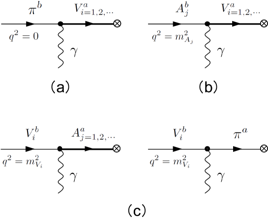
Figure 1: Diagrams contributing to the matrix elements: (a) $\langle 0|j_{\mu}^{a}|\pi^{b}\rangle_{\tilde{F}}$, (b) $\langle 0|j_{\mu}^{a}|A_{j}^{b}\rangle_{\tilde{F}}$, and (c) $\langle 0|j_{\mu}^{5a}|V_{i}^{b}\rangle_{\tilde{F}}$.

These sum rules also fix the matrix elements of the vector and axial currents between the vacuum and one particle state (a pion, a vector meson, or an axial-vector meson) in the presence of the soft electromagnetic field depicted in Fig. 1. Substituting Eqs. (47) and (48) into the definitions of $w_{L}$ and $w_{T}$ in Eq. (4), decomposing them into the sum over $i$ or $j$, and then using the sum rules, one finds

$$\langle 0|j_{\mu}^{a}(0)|\pi^{b}(q)\rangle_{\tilde{F}} = iq^{\nu}\frac{N_{c}}{2\pi^{2}f_{\pi}}d^{ab}{\tilde{F}}_{\mu\nu},$$ (53)

$$\langle 0|j_{\mu}^{a}(0)|A_{j}^{b}(q,\epsilon)\rangle_{\tilde{F}} = -\epsilon^{\alpha}\left(\eta_{\mu}^{\beta}-\frac{q_{\mu}q^{\beta}}{m_{A_{j}}^{2}}\right)\frac{N_{c}}{4\pi^{2}f_{\pi}^{2}}g_{A_{j}}d^{ab}{\tilde{F}}_{\alpha\beta},$$ (54)

$$\langle 0|j_{\mu}^{5a}(0)|V_{i}^{b}(q,\epsilon)\rangle_{\tilde{F}} = -\epsilon^{\alpha}\left[\left(\eta_{\mu}^{\beta}-\frac{q_{\mu}q^{\beta}}{m_{V_{i}}^{2}}\right)\frac{N_{c}}{4\pi^{2}f_{\pi}^{2}}g_{V_{i}}-\frac{q_{\mu}q^{\beta}}{m_{V_{i}}^{2}}f_{\pi}g_{\gamma V_{i}\pi}\right]d^{ab}{\tilde{F}}_{\alpha\beta}.$$ (55)

While Eq. (53) will be related to the well-known $\pi_{0}\rightarrow 2\gamma$ decay if one replaces the vector current by an on-shell photon, Eqs. (54) and (55) are the new formulas involving resonances. Remarkably, for fixed isospins $a$ and $b$, the transverse parts of the matrix elements (54) and (55) are respectively proportional to the decay constants $g_{V_{i}}$ and $g_{A_{j}}$ with the universal proportionality coefficient independent of species $i$ and $j$ (apart from the transverse projection). For example, for $N_{f}=2$, one has

$$\langle 0|j_{\mu}^{a}|\pi^{a}\rangle_{\tilde{F}}^{\parallel} = \mathop{\mathrm{tr}}[{\cal Q}]\frac{N_{c}}{8\pi^{2}f_{\pi}^{2}}{\tilde{F}}_{\mu\nu}\langle 0|j^{\nu 5a}|\pi^{a}\rangle,$$ (56)

$$\langle 0|j_{\mu}^{a}|A_{j}^{a}\rangle_{\tilde{F}}^{\perp} = \mathop{\mathrm{tr}}[{\cal Q}]\frac{N_{c}}{16\pi^{2}f_{\pi}^{2}}{\tilde{F}}_{\mu\nu}\langle 0|j^{\nu 5a}|A_{j}^{a}\rangle,\qquad(j=1,2,\cdots),$$ (57)

$$\langle 0|j_{\mu}^{5a}|V_{i}^{a}\rangle_{\tilde{F}}^{\perp} = \mathop{\mathrm{tr}}[{\cal Q}]\frac{N_{c}}{16\pi^{2}f_{\pi}^{2}}{\tilde{F}}_{\mu\nu}\langle 0|j^{\nu a}|V_{i}^{a}\rangle,\qquad(i=1,2,\cdots),$$ (58)

where no summation is taken over $a$. We note here that the universality of the proportionality coefficient originates from the constant value $-N_{c}/f_{\pi}^{2}$ with no $Q^{2}$-dependence in front of the bracket in Eq. (33).

The above sum rules and resultant matrix elements are generic to any theory with a Yang-Mills-Chern-Simons gravity dual in the large $N_{c}$ limit. As an example, we explicitly check the sum rules using the “cosh” model Son:2003et in Appendix A. However, they will not be generally valid in a theory incorporating the scalar field corresponding to the chiral condensate Erlich:2005qh ; Da Rold:2005zs ; Karch:2006pv (although we have a different type of sum rules which may be irrelevant to real QCD). We provide this counterexample in Appendix B. In the next section, we will discuss that real QCD behaves similarly to the former class of theories with the universality rather than to the latter counterexample.

If one assumes that sum rules (51) and (52) are saturated by the lowest resonances $i=j=1$, one has

$$g_{V_{1}} = g_{A_{1}},$$ (59)

$$g_{\gamma{V_{1}}{A_{1}}} = -\frac{N_{c}}{4\pi^{2}f_{\pi}^{2}}(m_{A_{1}}^{2}-m_{V_{1}}^{2}).$$ (60)

Equation (59) is equivalent to the second Weinberg sum rule $g_{V_{1}}^{2}-g_{A_{1}}^{2}=0$ Weinberg:1967kj , whereas Eq. (60) is a new prediction. Taking experimental values for these parameters, we find $g_{\gamma{\rho}{f_{1}}}\approx-9.2$ (and $g_{\gamma{\rho}{a}}\approx-8.0$) for $N_{c}=3$. This is not far from the value $|g_{\gamma{\rho}{f_{1}}}|=7.6\pm 1.1$ determined from the experimentally measured decay rate $\Gamma_{\rm exp}(f_{1}\rightarrow\rho^{0}+\gamma)=1.34\pm 0.38$ MeV PDG:2010 by using the formula Kochelev:1999zf :

$$\Gamma(f_{1}\rightarrow\rho^{0}+\gamma)=\frac{\alpha d_{30}^{2}g_{\gamma\rho f_{1}}^{2}}{24}\frac{(m_{f_{1}}^{2}+m_{\rho}^{2})(m_{f_{1}}^{2}-m_{\rho}^{2})^{3}}{m_{\rho}^{2}m_{f_{1}}^{5}},$$ (61)

where $d_{30}=1/4$ for ${\cal Q}={\rm diag}({2}/{3},-{1}/{3})$.

IV Real QCD

Let us discuss whether the relation (33) is realized in real QCD. This is easy to check for $Q^{2}\ll\Lambda_{\rm QCD}^{2}$ where the dynamics is governed by the low-lying pions. Because pions do not contribute to $w_{T}$, the left hand side of (33) should vanish at small $Q^{2}$. In the right hand side, pions only contribute to the axial correlator $\Pi_{A}\simeq f_{\pi}^{2}/Q^{2}$; the singularities of $1/Q^{2}$ cancel in total, and hence, Eq. (33) is valid.

In the opposite regime, $Q^{2}\gg\Lambda_{\rm QCD}^{2}$, one can make use of the operator product expansion (OPE) analysis, which is an expansion of the correlator in terms of $\Lambda_{\rm QCD}^{2}/Q^{2}$. As usually adopted in the practical applications of the QCD sum rules Shifman:1978bx , we shall neglect the $\alpha_{s}$-corrections and the anomalous dimensions of local composite operators in the OPE. Although these simplifications (called the practical OPE) are numerically good Shifman:1998rb , our discussion below is approximate at this level.

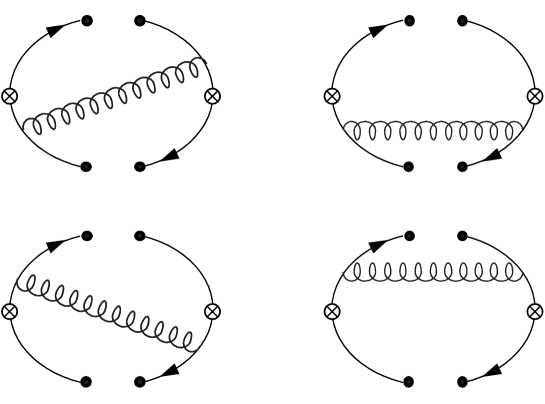
Figure 2: Diagrams contributing to $\langle j_{\mu}j_{\nu}^{5}\rangle_{\hat{F}}^{\rm nonpert}$. The solid and spiral lines denote quarks and gluons respectively.

For convenience, look at the relation (34) instead of (33). Because of the transformation properties under the $\text{SU}(N_{f})_{L}\times\text{SU}(N_{f})_{R}$ symmetry and the Lorentz symmetry, only the nonperturbative Lorentz pseudo-tensor condensates related to chiral symmetry breaking can appear in the OPE of $\langle j_{\mu}^{L}j_{\nu}^{R}\rangle_{\hat{F}}$. The leading contributions shown in Fig. 2 read Knecht:2002hr ; Czarnecki:2002nt

$$\langle j_{\mu}^{L}j_{\nu}^{R}\rangle_{\hat{F}}=\frac{1}{2}\langle j_{\mu}j_{\nu}^{5}\rangle_{\hat{F}}^{\rm nonpert}=-\frac{2g^{2}}{Q^{6}}(-q^{2}O_{\mu\nu}+q_{\mu}q^{\sigma}O_{\sigma\nu}-q_{\nu}q^{\sigma}O_{\sigma\mu}),$$ (62)

where $g$ is the QCD coupling constant and $O_{\mu\nu}=\langle(\bar{q}\gamma_{\mu}\gamma_{5}\lambda^{a}q)(\bar{q}\gamma_{\nu}\lambda^{a}q)\rangle$ is the four-quark condensate with the $\text{SU}(N_{c})$ color generators $\lambda^{a}$ ($a=1,2,\cdots,N_{c}^{2}-1$). Using the Fierz transformation together with the factorization of the four-quark condensate (which can be justified in the large $N_{c}$ limit), one has

$$O_{\mu\nu}=-\frac{N_{c}^{2}-1}{8N_{c}^{2}}\epsilon_{\mu\nu\alpha\beta}\langle\bar{q}q\rangle\langle\bar{q}\sigma^{\alpha\beta}q\rangle.$$ (63)

If we further use the magnetic susceptibility of the chiral condensate $\chi$ defined by Ioffe:1983ju

$$\langle\bar{q}\sigma_{\mu\nu}q\rangle=\chi\langle\bar{q}q\rangle\hat{F}_{\mu\nu},$$ (64)

Equation (62) reduces to the simple form:

$$\langle j_{\mu}^{L}j_{\nu}^{R}\rangle_{\hat{F}}=\frac{N_{c}^{2}-1}{2N_{c}^{2}}\frac{g^{2}}{Q^{4}}\chi\langle\bar{q}q\rangle^{2}P_{\mu}^{\alpha\perp}P_{\nu}^{\beta\perp}\tilde{F}_{\alpha\beta}.$$ (65)

On the other hand, the leading term in the OPE of $\Pi_{LR}$ is Shifman:1978bx

$$\Pi_{LR}(Q^{2})=-\frac{g^{2}}{Q^{6}}\langle(\bar{q}_{L}\gamma_{\mu}\lambda^{a}q_{L})(\bar{q}_{R}\gamma_{\mu}\lambda^{a}q_{R})\rangle=\frac{N_{c}^{2}-1}{4N_{c}^{2}}\frac{g^{2}}{Q^{6}}\langle\bar{q}q\rangle^{2}.$$ (66)

From Eqs. (65) and (66), that the relation (34) holds in QCD at large $Q^{2}$ amounts to the condition for $\chi$ to take a special value:

$$\chi=-\frac{N_{c}}{4\pi^{2}f_{\pi}^{2}}.$$ (67)

Interestingly, this is the same value obtained in another way assuming the pion dominance in the OPE of $w_{L}$ when one turns on the quark masses Vainshtein:2002nv (see Appendix C). These results suggest that the relation (33) is valid at least approximately in real QCD at both small and large $Q^{2}$.

V Conclusions

In this paper, we have shown a relation for the transverse part of triangle anomalies (the “anomaly matching for resonances”) in holographic QCD. Our relation provides a set of sum rules involving the masses, decay constants and couplings between resonances, and leads to the formulas for the matrix elements of the vector and axial currents in the presence of the soft electromagnetic field. These results are generic to any theory with a Yang-Mills-Chern-Simons gravity dual where chiral symmetry is broken by the boundary conditions.

In real QCD, our relation is also valid at least approximately when the magnetic susceptibility of the chiral condensate takes a special value $\chi=-N_{c}/(4\pi^{2}f_{\pi}^{2})$. The uncertainty of our relation in real QCD should be resolved in the future. This is relevant to the theoretical estimate of the hadronic electroweak contribution concerning $\gamma\gamma^{*}Z$ triangle diagrams to the muon anomalous magnetic moment, which can be experimentally determined to high precision Miller:2007kk ; Jegerlehner:2009ry .

There are several open questions. Among others, it is desirable to understand our relation and resulting formulas for the matrix elements in the field theoretical point of view. One can also consider its generalization to nonzero temperature and/or nonzero baryon chemical potential. In relation to heavy ion physics, this may lead to some possible effects on the “chiral magnetic effect” Kharzeev:2007jp ; Fukushima:2008xe considered to explain the fluctuations of charge asymmetry in noncentral collisions.

Appendix A Summary of results for the “cosh” model

In this appendix, we explicitly check our formulas in Sec. III using the “cosh” model as an example Son:2003et :

$$g(z) = g_{5}={\rm const},$$ (68)

$$f(z) = \frac{\Lambda}{g_{5}}\cosh(z),$$ (69)

and $z_{0}=\infty$. For completeness, we first review the results obtained in Son:2003et . To match the notation, we assign the integer $n$ to $V_{i}$ and $A_{j}$ with $n=2i-1$ for odd $n$ and $n=2j$ for even $n$ (due to the alternate states with the opposite parity). Then the results in Son:2003et are

$$b_{n}(z)=(-1)^{n}g_{5}c_{n}\frac{P_{n}^{1}(\tanh z)}{\cosh z},\qquad c_{n}=\sqrt{\frac{2n+1}{2n(n+1)}},$$ (70)

$$m_{n}^{2}=n(n+1)\Lambda^{2},$$ (71)

$$g_{n}=\sqrt{2n(n+1)(2n+1)}\frac{\Lambda^{2}}{g_{5}},$$ (72)

$$f_{\pi}^{2}=\frac{2\Lambda^{2}}{g_{5}^{2}},$$ (73)

$$\frac{1}{g_{5}^{2}}=\frac{N_{c}}{24\pi^{2}},$$ (74)

where $P_{n}^{1}(z)$ are the associated Legendre functions. We then summarize the new results using the formulas in Sec. III. Introducing the variables $y=\tanh z$ and $\nu$ satisfying $\nu(\nu+1)=-Q^{2}$, the solutions to the field equations (14) and (15) are

$$V(Q,z) = -\frac{\pi}{2}\sec(\nu\pi)\sqrt{1-y^{2}}[P_{\nu}^{1}(y)+P_{\nu}^{1}(-y)],$$ (75)

$$A(Q,z) = \frac{\pi}{2}\sec(\nu\pi)\sqrt{1-y^{2}}[P_{\nu}^{1}(y)-P_{\nu}^{1}(-y)],$$ (76)

where $\sec t\equiv 1/\cos t$. The relations (31) and (32) are

$$\Pi_{A}(Q^{2})-\Pi_{V}(Q^{2}) = \frac{N_{c}}{12\pi}\sec\left(\frac{\pi}{2}\sqrt{1-\frac{4Q^{2}}{\Lambda^{2}}}\right)$$ (77)

$$= \left\{\begin{array}[]{ll}\displaystyle{\frac{N_{c}}{6\pi}}e^{-\pi{Q}/{\Lambda}},&Q^{2}\gg\Lambda^{2},\rule[-15.0pt]{0.0pt}{15.0pt}\\ \displaystyle{\frac{N_{c}}{12\pi^{2}}}\displaystyle{\frac{\Lambda^{2}}{Q^{2}}},&Q^{2}\ll\Lambda^{2},\end{array}\right.$$ (80)

$$w_{T}(Q^{2}) = \frac{N_{c}}{Q^{2}}\left[1-\pi\frac{Q^{2}}{\Lambda^{2}}\sec\left(\frac{\pi}{2}\sqrt{1-\frac{4Q^{2}}{\Lambda^{2}}}\right)\right]$$ (81)

$$= \left\{\begin{array}[]{ll}\displaystyle{\frac{N_{c}}{Q^{2}}}-\displaystyle{\frac{2\pi N_{c}}{\Lambda^{2}}}e^{-\pi{Q}/{\Lambda}},&Q^{2}\gg\Lambda^{2},\rule[-15.0pt]{0.0pt}{15.0pt}\\ \displaystyle{\frac{N_{c}}{\Lambda^{2}}},&Q^{2}\ll\Lambda^{2},\end{array}\right.$$ (84)

Therefore, the following relation is actually satisfied:

$$w_{T}(Q^{2})=\frac{N_{c}}{Q^{2}}-\frac{N_{c}}{f_{\pi}^{2}}\left[\Pi_{A}(Q^{2})-\Pi_{V}(Q^{2})\right].$$ (85)

For the couplings $g_{\gamma V_{i}\pi}$ and $g_{\gamma V_{i}A_{j}}$, which we denote $g_{\gamma n\pi}$ and $g_{\gamma nm}$ with $n=2i-1$ and $m=2j$, there are the “neighboring rules”:

$$g_{\gamma n\pi}=\frac{4\sqrt{3}}{g_{5}f_{\pi}}\delta_{n1},$$ (86)

$$g_{\gamma nm}=-6(n+1)\sqrt{\frac{n(n+2)}{(2n+1)(2n+3)}}\delta_{n,m-1}+6n\sqrt{\frac{(n-1)(n+1)}{(2n-1)(2n+1)}}\delta_{n,m+1}.$$ (87)

Using the above relations, one can easily check the longitudinal and transverse sum rules:

$$\frac{g_{\gamma 1\pi}g_{1}}{m_{1}^{2}}=\frac{N_{c}}{2\pi^{2}f_{\pi}},$$ (88)

$$\sum_{m=n\pm 1}\frac{{g_{\gamma nm}}g_{m}}{m_{m}^{2}-m_{n}^{2}}=-\frac{3}{g_{5}}\sqrt{2n(n+1)(2n+1)}=-\frac{N_{c}}{4\pi^{2}f_{\pi}^{2}}g_{n},$$ (89)

$$\sum_{n=m\pm 1}\frac{{g_{\gamma nm}}g_{n}}{m_{m}^{2}-m_{n}^{2}}=-\frac{3}{g_{5}}\sqrt{2m(m+1)(2m+1)}=-\frac{N_{c}}{4\pi^{2}f_{\pi}^{2}}g_{m}.$$ (90)

Appendix B AdS/QCD with the chiral condensate

One can test whether the relation (33) is realized in the AdS/QCD incorporating the chiral condensate Erlich:2005qh ; Da Rold:2005zs ; Karch:2006pv . We consider the hard-wall model and follow the notations of Erlich:2005qh . The metric is a slice of anti-de Sitter (AdS) space:

$$ds^{2}=\frac{1}{z^{2}}(-dz^{2}+dx^{\mu}dx_{\mu}),\qquad 0<z\leq z_{m}.$$ (91)

The IR cutoff $z_{m}$ is responsible for the confinement and fixes the scale of the $\rho$ meson mass $m_{\rho}$ in this theory. When we are interested in the physics at large $Q^{2}$ below, we can limit ourselves to the region of AdS space close to the boundary and we can take the $z_{m}\rightarrow\infty$ limit to simplify the computation.

The action of the theory in the 5D bulk is

$$S = S_{\rm YM}+S_{\rm CS},$$ (92)

$$S_{\rm YM} = \int\!d^{5}x\,\sqrt{g}\mathop{\mathrm{tr}}{\left[|DX|^{2}+3|X|^{2}-\frac{1}{4g_{5}^{2}}(F_{L}^{2}+F_{R}^{2})\right]},$$ (93)

$$S_{\rm CS} = \kappa\int[w_{5}(A_{L})-w_{5}(A_{R})],$$ (94)

where $D_{\mu}X=\partial_{\mu}X-iA_{L\mu}X+iXA_{R\mu}$, $A_{L,R}=A_{L,R}^{a}\tau^{a}$, $F_{\mu\nu}=\partial_{\mu}A_{\nu}-\partial_{\nu}A_{\mu}-i[A_{\mu},A_{\nu}]$, and $w(A)=AF^{2}-\frac{i}{2}A^{3}F-\frac{1}{10}A^{5}$. The coefficient $\kappa$ is fixed in Eq. (29). The expectation value of the scalar field $X$ is determined by the classical solution as

$$X_{0}(z)=\frac{1}{2}m_{q}z+\frac{1}{2}\sigma z^{3}.$$ (95)

In the following, we consider the chiral limit $m_{q}=0$.

We introduce the vector and axial-vector fields $V=(A_{L}+A_{R})/2$ and $A=(A_{L}-A_{R})/2$ and we work in the $V_{z}=A_{z}=0$ gauge, letting $V^{\mu}(q,z)=V(q,z)V_{0}^{\mu}(q)$ with $V_{0}$ being the source of the vector current (likewise for $A_{\mu}$). The linearized equations of motion for the transverse parts $V_{\perp}(q,z)$ and $A_{\perp}(q,z)$ are

$$\left(\frac{V_{\perp}^{\prime}}{z}\right)^{\prime}-\frac{Q^{2}}{z}V_{\perp}=0,$$ (96)

$$\left(\frac{A_{\perp}^{\prime}}{z}\right)^{\prime}-\frac{Q^{2}}{z}A_{\perp}-\frac{g_{5}^{2}v^{2}}{z^{3}}A_{\perp}=0,$$ (97)

with the boundary conditions $V(Q,\epsilon)=A(Q,\epsilon)=1$ and $V^{\prime}(Q,z_{m})=A^{\prime}(Q,z_{m})=0$. One can also write down the equation of motion for the longitudinal part $A_{\parallel}$, but it is irrelevant to our discussion and is omitted here.

Equation (96) can be solved analytically,

$$V_{\perp}(Q,z)=Qz\left[K_{1}(Qz)+I_{1}(Qz)\frac{K_{0}(Qz_{m})}{I_{0}(Qz_{m})}\right]\xrightarrow{z_{m}\to\infty}QzK_{1}(Qz),$$ (98)

where $K_{n}$ and $I_{n}$ are the modified Bessel functions. Although Eq. (97) does not allow for an analytical solution generally, one can solve perturbatively for large $Q^{2}$,

$$A_{\perp}=A_{0}+A_{1}+\dots,$$ (99)

with $A_{0}(Q,z)=V_{\perp}(Q,z)$. The first correction satisfies

$$\partial_{x}^{2}A_{1}-\frac{1}{x}\partial_{x}A_{1}-A_{1}=\lambda x^{4}A_{0},$$ (100)

where we define $x\equiv Qz$ and $\lambda\equiv g_{5}^{2}\sigma^{2}/Q^{6}$. The solution to this equation is given by using the Green’s function,

$$A_{1}(x)=\int\!dx^{\prime}\,G(x,x^{\prime})\lambda x^{\prime 4}A_{0}(x^{\prime}),$$ (101)

where $G(x,x^{\prime})$ can be obtained from the solutions to the homogeneous part of Eq. (100),

$$f_{1}(x)=xK_{1}(x),\qquad f_{2}(x)=xI_{1}(x),$$ (102)

as

$$G(x,x^{\prime})=-\frac{1}{W[f_{1},f_{2}](x^{\prime})}[f_{1}(x)f_{2}(x^{\prime})\theta(x-x^{\prime})+f_{2}(x)f_{1}(x^{\prime})\theta(x^{\prime}-x)],$$ (103)

with the Wronskian $W[f_{1},f_{2}](x^{\prime})\equiv f_{1}f_{2}^{\prime}-f_{1}^{\prime}f_{2}=x^{\prime}$. Using the integral,

$$\int_{0}^{\infty}\!dx^{\prime}\,x^{\prime 5}K_{1}^{2}(x^{\prime})=\frac{8}{5},$$ (104)

we find the small $z$ behavior of $A_{1}$:

$$A_{1}(Q,z)=-\frac{4}{5}(Qz)^{2}\frac{g_{5}^{2}\sigma^{2}}{Q^{6}}.$$ (105)

This solution near the boundary is sufficient to evaluate the correlation functions below which are determined by the boundary values at $z=\epsilon$ or by the integrals dominated by small $z$ regions.

The derivations of the correlation functions are similar to those in Sec. III and we simply denote the resultant expressions here. The transverse parts of the vector and axial current correlation functions are

$$\Pi_{V}(Q^{2}) = \left.-\frac{1}{g_{5}^{2}Q^{2}}\frac{V_{\perp}^{\prime}(Q,z)}{z}\right|_{z=\epsilon},$$ (106)

$$\Pi_{A}(Q^{2}) = \left.-\frac{1}{g_{5}^{2}Q^{2}}\frac{A_{\perp}^{\prime}(Q,z)}{z}\right|_{z=\epsilon},$$ (107)

Since $\Pi_{A}(Q^{2})\rightarrow f_{\pi}^{2}/Q^{2}$ for $Q^{2}\rightarrow 0$, the pion decay constant reads

$$f_{\pi}^{2}=\left.-\frac{1}{g_{5}^{2}}\frac{A_{\perp}^{\prime}(0,z)}{z}\right|_{z=\epsilon}.$$ (108)

The expressions for $w_{L}$ and $w_{T}$ are

$$w_{L}(Q^{2}) = -\frac{2N_{c}}{Q^{2}}\int_{0}^{z_{m}}\!dz\,A_{\perp}^{\prime}(0,z)V_{\perp}(0,z)\xrightarrow{z_{m}\to\infty}\frac{2N_{c}}{Q^{2}},,$$ (109)

$$w_{T}(Q^{2}) = -\frac{2N_{c}}{Q^{2}}\int_{0}^{z_{m}}\!dz\,A_{\perp}(Q,z)V_{\perp}^{\prime}(Q,z),$$ (110)

where we used $V_{\perp}(0,z)=1$. The result for $w_{L}$ is consistent with the anomaly matching condition (5).

Now we are ready to check the validity of the relation (33) in this theory. Let us first consider small $Q^{2}$. Using $V(0,z)=1$, one can easily check that $\Pi_{V}$ and $w_{T}$ vanish while $\Pi_{A}(Q^{2})\rightarrow f_{\pi}^{2}/Q^{2}$; thus the relation (33) is valid.

On the other hand, for large $Q^{2}$, we can expand $V_{\perp}$ and $A_{\perp}$ near the boundary,

$$V_{\perp}(Q,z) = 1+\frac{1}{4}(Qz)^{2}\ln(Q^{2}z^{2})+\dots,$$ (111)

$$A_{\perp}(Q,z) = 1+\frac{1}{4}(Qz)^{2}\ln(Q^{2}z^{2})-\frac{4}{5}(Qz)^{2}\frac{g_{5}^{2}\sigma^{2}}{Q^{6}}+\dots,$$ (112)

which lead to (up to contact terms):

$$\Pi_{V}(Q^{2}) = -\frac{1}{2g_{5}^{2}}\ln Q^{2},$$ (113)

$$\Pi_{A}(Q^{2}) = -\frac{1}{2g_{5}^{2}}\ln Q^{2}+\frac{8}{5}\frac{\sigma^{2}}{Q^{6}},$$ (114)

$$w_{T}(Q^{2}) = \frac{N_{c}}{Q^{2}}-\frac{32N_{c}}{5}\frac{g_{5}^{2}\sigma^{2}}{Q^{8}},$$ (115)

where the integral

$$\int_{0}^{\infty}\!dx\,x^{2}K_{1}(x)=2,$$ (116)

is used for evaluating $w_{T}$. Matching the leading log behavior in Eq. (113) with the QCD result:

$$\Pi_{V}(Q^{2})=-\frac{N_{c}}{24\pi^{2}}\ln Q^{2},$$ (117)

leads to the identification Erlich:2005qh :

$$g_{5}^{2}=\frac{12\pi^{2}}{N_{c}}.$$ (118)

Combining the above results, one arrives at

$$w_{T}(Q^{2})=\frac{N_{c}}{Q^{2}}-\frac{48\pi^{2}}{Q^{2}}[\Pi_{A}(Q^{2})-\Pi_{V}(Q^{2})],$$ (119)

for large $Q^{2}$. Clearly, the nonperturbative correction is different from Eq. (33) and from the behavior in real QCD shown in Sec. IV: the coefficient in front of the bracket is $Q^{2}$-dependent but not a constant $-N_{c}/f_{\pi}^{2}$. This difference originates from the OPE of $w_{T}$ in Eq. (115) where the nonperturbative correction is proportional to $1/Q^{8}$ rather than $1/(f_{\pi}^{2}Q^{6})$. This will be due the absence of the field corresponding to the operator $\bar{q}\sigma_{\mu\nu}q$ in this theory which is essential for the relation (33) to be realized in real QCD at large $Q^{2}$. One may improve this point by adding the tensor field $H_{\mu\nu}$ corresponding to the operator $\bar{q}\sigma_{\mu\nu}q$ in the theory, although it would still require a fine-tuning of parameters to reproduce the quantitatively correct OPE in QCD.

In this case, one can still derive a set of transverse sum rules [but different type from Eqs. (51) and (52)] for highly excited resonances using Eq. (119). Since pions do not contribute to $w_{T}$, we have only to consider the contributions from the vector and axial-vector mesons for $w_{T}$. Similarly to Eq. (50), one obtains a relation:

$$\sum_{i,j}g_{\gamma{V_{i}}{A_{j}}}\frac{g_{V_{i}}}{Q^{2}+m_{V_{i}}^{2}}\frac{g_{A_{j}}}{Q^{2}+m_{A_{j}}^{2}} = 12\sum_{i,j}\left[\frac{g_{V_{i}}^{2}}{m_{V_{i}}^{2}(Q^{2}+m_{V_{i}}^{2})}-\frac{g_{A_{j}}^{2}}{m_{A_{j}}^{2}(Q^{2}+m_{A_{j}}^{2})}\right]$$ (120)

$$-\frac{12f_{\pi}^{2}}{Q^{2}}+\frac{N_{c}}{4\pi^{2}},$$

for sufficiently large $Q^{2}$. This provides a set of sum rules for highly excited states:

$$\sum_{j}\frac{{g_{\gamma V_{i}A_{j}}}g_{A_{j}}}{m_{A_{j}}^{2}-m_{V_{i}}^{2}} = 12\frac{g_{V_{i}}}{m_{V_{i}}^{2}},\qquad(i\gg 1),$$

$$\sum_{i}\frac{{g_{\gamma V_{i}A_{j}}}g_{V_{i}}}{m_{A_{j}}^{2}-m_{V_{i}}^{2}} = 12\frac{g_{A_{j}}}{m_{A_{j}}^{2}},\qquad(j\gg 1).$$ (121)

They also lead to the relations for the transverse parts of the matrix elements:

$$\langle 0|j_{\mu}^{5a}|V_{i}^{b}\rangle_{\tilde{F}}^{\perp} = 12\epsilon^{\alpha}\frac{g_{V_{i}}}{m_{V_{i}}^{2}}d^{ab}{\tilde{F}}_{\alpha\beta},\qquad(i\gg 1),$$ (122)

$$\langle 0|j_{\mu}^{a}|A_{j}^{b}\rangle_{\tilde{F}}^{\perp} = 12\epsilon^{\alpha}\frac{g_{A_{j}}}{m_{A_{j}}^{2}}d^{ab}{\tilde{F}}_{\alpha\beta},\qquad(j\gg 1).$$ (123)

These matrix elements are proportional not only to the decay constants $g_{V_{i}}$ and $g_{A_{j}}$ but also to $1/m_{V_{i}}^{2}$ and $1/m_{A_{j}}^{2}$, respectively: there is no universality of the proportionality coefficients unlike Eqs. (54) and (55). This again comes from the $1/Q^{2}$ behavior in front of the bracket in Eq. (119), and is different from real QCD where this factor should be approximately replaced by a constant value. Therefore, we expect that real QCD would have the properties (54) and (55) rather than (122) and (123).

Appendix C Magnetic susceptibility of the chiral condensate

In this appendix, we review the derivation of the magnetic susceptibility of the chiral condensate by Vainshtein Vainshtein:2002nv . Let us consider the modifications of the longitudinal part of the correlator (4) when we turn on the degenerate quark masses $m_{q}$. For $Q^{2}\gg\Lambda_{\rm QCD}^{2}$, the leading contribution can be found using the OPE,

$$\langle j_{\mu}j_{\nu}^{5}\rangle_{\hat{F}}^{\parallel} = Q^{2}P_{\mu}^{\alpha\perp}P_{\nu}^{\beta\parallel}\epsilon_{\alpha\beta\rho\sigma}\left[\frac{N_{c}}{4\pi^{2}Q^{2}}\hat{F}^{\rho\sigma}-\frac{2m_{q}\langle\bar{q}\sigma^{\rho\sigma}q\rangle}{Q^{4}}+{\cal O}\left(\frac{1}{Q^{6}}\right)\right]$$ (124)

$$= \frac{Q^{2}}{4\pi^{2}}P_{\mu}^{\alpha\perp}P_{\nu}^{\beta\parallel}\tilde{F}_{\alpha\beta}\left[\frac{2N_{c}}{Q^{2}}-\frac{16\pi^{2}\chi m_{q}\langle\bar{q}q\rangle}{Q^{4}}+{\cal O}\left(\frac{1}{Q^{6}}\right)\right],$$

where we used the definition of $\chi$ in Eq. (67). For $Q^{2}\ll\Lambda_{\rm QCD}^{2}$, the pion propagator is replaced by the massive one:

$$\langle j_{\mu}j_{\nu}^{5}\rangle_{\hat{F}}^{\parallel} = \frac{Q^{2}}{4\pi^{2}}P_{\mu}^{\alpha\perp}P_{\nu}^{\beta\parallel}\tilde{F}_{\alpha\beta}\frac{2N_{c}}{Q^{2}+m_{\pi}^{2}}$$ (125)

$$= \frac{Q^{2}}{4\pi^{2}}P_{\mu}^{\alpha\perp}P_{\nu}^{\beta\parallel}\tilde{F}_{\alpha\beta}\left[\frac{2N_{c}}{Q^{2}}-\frac{2N_{c}m_{\pi}^{2}}{Q^{4}}+{\cal O}\left(\frac{1}{Q^{6}}\right)\right].$$

If one assumes the extrapolation of the $1/Q^{4}$ term in the bracket in Eq. (125) to large $Q^{2}$ to be matched against that in Eq. (124), one finds

$$\chi=\frac{N_{c}m_{\pi}^{2}}{8\pi^{2}m_{q}\langle\bar{q}q\rangle}.$$ (126)

Using the Gell-Mann–Oakes–Renner relation for pions,

$$f_{\pi}^{2}m_{\pi}^{2}=-2m_{q}\langle\bar{q}q\rangle,$$ (127)

Equation (126) reduces to

$$\chi=-\frac{N_{c}}{4\pi^{2}f_{\pi}^{2}}.$$ (128)

References

- (1) S. L. Adler, Phys. Rev. 177, 2426 (1969).
- (2) J. S. Bell and R. Jackiw, Nuovo Cim. A 60 (1969) 47.
- (3) S. L. Adler and W. A. Bardeen, Phys. Rev. 182, 1517 (1969).
- (4) G. ’t Hooft, Recent Developments In Gauge Theories, (Plenum, New York, 1980).
- (5) A. Vainshtein, Phys. Lett. B 569, 187 (2003) [arXiv:hep-ph/0212231].
- (6) A. Czarnecki, W. J. Marciano and A. Vainshtein, Phys. Rev. D 67, 073006 (2003) [Erratum-ibid. D 73, 119901 (2006)] [arXiv:hep-ph/0212229].
- (7) M. Knecht, S. Peris, M. Perrottet and E. de Rafael, JHEP 0403, 035 (2004) [arXiv:hep-ph/0311100].
- (8) J. Maldacena, Adv. Theor. Math. Phys. 2, 231 (1998) [Int. J. Theor. Phys. 38, 1113 (1999)] [arXiv:hep-th/9711200].
- (9) S. S. Gubser, I. R. Klebanov and A. M. Polyakov, Phys. Lett. B 428, 105 (1998) [arXiv:hep-th/9802109].
- (10) E. Witten, Adv. Theor. Math. Phys. 2, 253 (1998) [arXiv:hep-th/9802150].
- (11) D. T. Son and M. A. Stephanov, Phys. Rev. D 69, 065020 (2004) [arXiv:hep-ph/0304182].
- (12) T. Sakai and S. Sugimoto, Prog. Theor. Phys. 113, 843 (2005) [arXiv:hep-th/0412141]; Prog. Theor. Phys. 114, 1083 (2005) [arXiv:hep-th/0507073].
- (13) A. Gorsky and A. Krikun, Phys. Rev. D 79, 086015 (2009) [arXiv:0902.1832 [hep-ph]].
- (14) J. Erlich, E. Katz, D. T. Son and M. A. Stephanov, Phys. Rev. Lett. 95, 261602 (2005) [arXiv:hep-ph/0501128].
- (15) L. Da Rold and A. Pomarol, Nucl. Phys. B 721, 79 (2005) [arXiv:hep-ph/0501218].
- (16) A. Karch, E. Katz, D. T. Son and M. A. Stephanov, Phys. Rev. D 74, 015005 (2006) [arXiv:hep-ph/0602229].
- (17) S. Weinberg, Phys. Rev. Lett. 18, 507 (1967).
- (18) S. K. Domokos, H. R. Grigoryan and J. A. Harvey, Phys. Rev. D 80, 115018 (2009) [arXiv:0905.1949 [hep-ph]].
- (19) K. Nakamura et al. (Particle Data Group), J. Phys. G 37, 075021 (2010).
- (20) N. I. Kochelev, D. P. Min, Y. s. Oh, V. Vento and A. V. Vinnikov, Phys. Rev. D 61, 094008 (2000) [arXiv:hep-ph/9911480].
- (21) M. A. Shifman, A. I. Vainshtein and V. I. Zakharov, Nucl. Phys. B 147, 385 (1979); Nucl. Phys. B 147, 448 (1979).
- (22) M. A. Shifman, Prog. Theor. Phys. Suppl. 131, 1 (1998) [arXiv:hep-ph/9802214].
- (23) M. Knecht, S. Peris, M. Perrottet and E. De Rafael, JHEP 0211, 003 (2002) [arXiv:hep-ph/0205102].
- (24) B. L. Ioffe and A. V. Smilga, Nucl. Phys. B 232, 109 (1984).
- (25) H. R. Grigoryan and A. V. Radyushkin, Phys. Rev. D 77, 115024 (2008) [arXiv:0803.1143 [hep-ph]].
- (26) J. P. Miller, E. de Rafael and B. L. Roberts, Rept. Prog. Phys. 70, 795 (2007) [arXiv:hep-ph/0703049].
- (27) F. Jegerlehner and A. Nyffeler, Phys. Rept. 477, 1 (2009) [arXiv:0902.3360 [hep-ph]].
- (28) D. E. Kharzeev, L. D. McLerran and H. J. Warringa, Nucl. Phys. A 803, 227 (2008) [arXiv:0711.0950 [hep-ph]].
- (29) K. Fukushima, D. E. Kharzeev and H. J. Warringa, Phys. Rev. D 78, 074033 (2008) [arXiv:0808.3382 [hep-ph]].