Two stochastic models of a random walk in the ${\mathrm{U}}(n)$-spherical duals of ${\mathrm{U}}(n+1)$

Abstract.

The random walk to be considered takes place in the $\delta$-spherical dual of the group ${\mathrm{U}}(n+1)$, for a fixed finite dimensional irreducible representation $\delta$ of ${\mathrm{U}}(n)$. The transition matrix comes from the three term recursion relation satisfied by a sequence of matrix valued orthogonal polynomials built up from the irreducible spherical functions of type $\delta$ of ${\mathrm{SU}}(n+1)$. One of the stochastic models is an urn model and the other is a Young diagram model.

1. Introduction

Around 1770 D. Bernoulli studied a model for the exchange of heat between two bodies. This model can also be seen as a description of the diffusion of a pair of incompressible gases between two containers. This model was independently analyzed by S. Laplace around 1810, see the references in [F]. Another model of similar characteristics was introduced by P. and T. Ehrenfest in 1907 in connection with the controversies surrounding the work of L. Boltzmann in the kinetic theory of gases dealing with reversibility and convergence to equilibrium. Boltzmann had apparentlly deduced his H-theorem dictating convergence to equilibrium starting from the time reversible equations of Newton. For a nice account of this see [K]. Both of these models are instances of discrete time Markov chains with fairly explicit tridiagonal one-step transition probability matrices which are obtained by considering carefully the underlying stochastic mechanism that connects the state of the system at two consecutive values of time.

The second model features two urns, I and II, that share a total of N balls. The state of the system at time $n$ is the number of balls in urn I. Each ball has a different label from the set $1,2,...,N$. At time $n$ a number $j$ in the set $1,2,...,N$ is chosen with equal probabilities and the ball with this label is moved from the urn where it sits to the other urn. This gives the state of the system at time $n+1$. Writing down the one-step transition probability matrix is now a matter of counting carefully.

While it had been possible to obtain interesting answers for these two models for quite some time, it is only much more recently that some very nice connections have been noticed between these models and some basic sets of discrete orthogonal polynomials, namely the Krawtchouk and the dual Hahn polynomials. Moreover although there are many ways of arriving at these polynomials it is relevant to mention here that they can be realized as the ”spherical functions” for certain finite bihomogeneous spaces. A very good reference for this material is [S]. We stress the remarkable fact that these two models of old vintage and clear physical significance can be solved in terms of the simplest of all hypergeometric functions, namely ${}_{2}F_{1}$ and ${}_{3}F_{2}$.

As many readers certainly know many of the classical special functions of mathematical physics, such as the Legendre, the Hermite and the Laguerre polynomials, could have been obtained for the first time as spherical functions for certain symmetric spaces. A good basic reference here is [V]. The way that things developed historically is, of course, completely different.

The interplay between important physical problems and certain tools that arise naturally in group representation theory constitutes the theme of this paper. The situation described here is the reverse of what has been discussed above for the Bernoulli-Laplace and the Ehrenfest models: we will go from group representation theory to some concrete models that might be of some physical interest. We will start from a matrix that is obtained from group representation theory and try to build a model that goes along with it. The models constructed here are certainly not the only possible ones. More natural ones might be lurking around.

In a series of papers including [T1, T2, GPT, GPT1, GPT2, GPT3, P, PT1, PT2, PT3, PT4] one considers matrix valued spherical functions associated to a pair $(G,K)$ arriving at sequences of matrix valued polynomials of one real variable satisfying a three term recursion relation whose semi-infinite block tridiagonal matrix is stochastic, i.e. the entries are non-negative and the sum of the elements in any row is $1$. This matrix depends on a number of free parameters that have a very definite group theoretical meaning. The important point is that the tools developed in the papers just mentioned allow one to give explicit expressions, in terms of some definite integrals, of all the entries of any power of the original matrix. This means that if one could think of a nice Markov chain with this matrix as its one-step transition probability matrix one would have an explicit form for the entries of the $n$-step transition probability matrix. Many readers will recognize that this is exactly what S. Karlin and J. McGregor, see [KMcG], proposed as a way of exploiting orthogonal polynomials and the role they play in the spectral analysis of certain finite or semi-infinite tridiagonal matrices. The method advocated in [KMcG] starts with a so called birth-and-death process whose one-step tridiagonal transition matrix is easily constructed from the given model and one has to look for the corresponding spectral information: the eigenfunctions and the spectral measure. Here we travel this road in the opposite direction in a more elaborate set-up.

The relation between matrix valued orthogonal polynomials, block tridiagonal matrices and Quasi-Birth and Death processes has been first exploited independently in [DRSZ, G] as well as in later papers by these authors.

We will consider several random walks whose configuration spaces are subsets of $\hat{\mathrm{U}}(n+1)({\mathbf{k}})$, the so call ${\mathbf{k}}$-spherical dual of ${\mathrm{U}}(n+1)$, and whose one-step transition matrices come from the stochastic matrix that appears in [PT2] and [P], see also [PT4]. The dual of ${\mathrm{U}}(n+1)$ is the set $\hat{\mathrm{U}}(n+1)$ of all equivalence classes of finite dimensional irreducible representations of ${\mathrm{U}}(n+1)$. These equivalence classes are parametrized by the $n+1$-tuples of integers ${\mathbf{m}}=(m_{1},\dots,m_{n+1})$ subject to the conditions $m_{1}\geq\cdots\geq m_{n+1}$.

If ${\mathbf{k}}=(k_{1},\cdots,k_{n})\in\hat{\mathrm{U}}(n)$, the ${\mathbf{k}}$-spherical dual of ${\mathrm{U}}(n+1)$ is the subset $\hat{\mathrm{U}}(n+1)({\mathbf{k}})$ of $\hat{\mathrm{U}}(n+1)$ of the representations of ${\mathrm{U}}(n+1)$ whose restriction to ${\mathrm{U}}(n)$ contains the representation ${\mathbf{k}}$. Then it is well known, see [V], that $\hat{\mathrm{U}}(n+1)({\mathbf{k}})$ corresponds to the set of all ${\mathbf{m}}$’s as above that satisfy the extra constraints

(1) $$m_{i}\geq k_{i}\geq m_{i+1},\quad\text{ for all}\quad i=1,\dots,n.$$

In other words $\hat{\mathrm{U}}(n+1)({\mathbf{k}})$ can be visualized as the subset of all points ${\mathbf{m}}$ of the integral lattice $\mathbb{Z}^{n+1}$ in the set

$$[k_{1},\infty)\times[k_{2},k_{1}]\times\cdots\times[k_{n-1},k_{n}]\times(-\infty,k_{n}].$$

An example is given in the figure below.

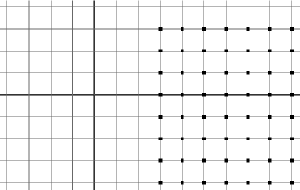
Figure 1. $\hat{\mathrm{U}}(n+1)({\mathbf{k}})$, $n=1$, $k_{1}=3$.

We can now state more precisely the point of this paper: starting from the stochastic matrix $M$ that appears in [PT2] and [P], we describe a random mechanism that gives rise to a Markov chain whose state space is the subset of $\hat{\mathrm{U}}(n+1)({\mathbf{k}})$ of all ${\mathbf{m}}\in\hat{\mathrm{U}}(n+1)({\mathbf{k}})$ such that $s_{{\mathbf{m}}}=s_{{\mathbf{k}}}$ and $k_{n}\geq 0$ ($s_{{\mathbf{m}}}=m_{1}+\cdots+m_{n+1},s_{{\mathbf{k}}}=k_{1}+\cdots+k_{n}$), and whose one-step transition matrix coincides with the one we started from. The construction in [GPT] and [PT2] deals with the case of $({\mathrm{SU}}(3),{\mathrm{U}}(2))$ but in [PT3] and [P] this was extended to the case of $({\mathrm{SU}}(n+1),{\mathrm{U}}(n))$.

One step of the Markov evolution will consist of two substeps taken in succesion. In the first substep one of the values of $m_{i}$ increases by one, subject to the constraints (1). In the second substep one of the new values of our $m_{i}$’s decreases by one, again this is subject to the same constraints. Thus from the configuration ${\mathbf{m}}$ one could for instance go to ${\mathbf{m}}-{\mathbf{e}}_{i}+{\mathbf{e}}_{j}$ or one could stay put at ${\mathbf{m}}$. We use the notation ${\mathbf{e}}_{i}$ for the vector with its $i$th component equal to $1$ and all the others equal to $0$. Any state has a total of at most $n(n+1)+1$ positions where it can move in one complete step of our process consisting of two simpler steps. Keep in mind that the two succesive simpler steps can end up with our random walker in the initial state. We will analyze in detail the simpler substeps that constitute one full step of our process. This will take up most of the analysis in the next sections.

We now describe the contents of the paper.

In Section 2 we collect the necessary material to state and explain a three term recursion relation (with matrix coefficients) for a sequence of matrix valued orthogonal polynomials, built up from irreducible spherical functions of a fixed type associated to the pair $({\mathrm{SU}}(n+1),{\mathrm{U}}(n))$. This should help the reader make the connection between [PT2, P] and the present paper.

In Section 3 we construct a factorization of the stochastic matrix that define the three term recursion relation for the sequence of matrix valued orthogonal polynomials given in the previous section. This factorization into two stochastic matrices leads to the two substeps mentioned above.

Before starting the analysis of our general urn model in Section 5 for one of the substeps, we describe in detail in Section 4 an urn model for $n=2$.

The definition of the stochastic matrix $M$ alluded above, as well as its factorization make sense for any ${\mathbf{m}}\in\hat{\mathrm{U}}(n+1)({\mathbf{k}})$.

To each configuration $m_{1}\geq m_{2}\geq\cdots\geq m_{n}\geq 0$ of $n$ integer numbers we associate its Young diagram, a combinatorial object which has $m_{1}$ boxes in the first row, $m_{2}$ boxes in the second row, and so on down to the last row which has $m_{n}$ boxes. For example the Young diagram associated to the configuration $6\geq 4\geq 4\geq 3$ is

$$\begin{array}[]{l}\begin{array}[]{|c|c|c|c|c|c|}\hline\cr\makebox[4.2679pt]{}&\makebox[4.2679pt]{}&\makebox[4.2679pt]{}&\makebox[4.2679pt]{}&\makebox[4.2679pt]{}&\makebox[4.2679pt]{}\\ \hline\cr\end{array}\\ \begin{array}[]{|c|c|c|c|}\makebox[4.2679pt]{}&\makebox[4.2679pt]{}&\makebox[4.2679pt]{}&\makebox[4.2679pt]{}\\ \hline\cr\end{array}\\ \begin{array}[]{|c|c|c|c|}\makebox[4.2679pt]{}&\makebox[4.2679pt]{}&\makebox[4.2679pt]{}&\makebox[4.2679pt]{}\\ \hline\cr\end{array}\\ \begin{array}[]{|c|c|c|}\makebox[4.2679pt]{}&\makebox[4.2679pt]{}&\makebox[4.2679pt]{}\\ \hline\cr\end{array}\\ \end{array}$$

Figure 2.

Young diagrams and their relatives the Young tableaux are very useful in representation theory. They provide a convenient way to describe the group representations of the symmetric and general linear groups and to study their properties. In particular Young diagrams are in one-to-one correspondence with the irreducible representations of the symmetric group over the complex numbers and the irreducible polynomial representations of the general linear groups. They were introduced by Alfred Young in 1900. They were then applied to the study of the symmetric group by Georg Frobenius in 1903. Their theory and applications were further developed by many mathematicians and there are numerous and interesting applications, beyond representation theory, in combinatorics and algebraic geometry.

If we consider the subset all ${\mathbf{m}}\in\hat{\mathrm{U}}(n+1)({\mathbf{k}})$ such that $m_{n+1}\geq 0$ it is natural to represent such a state of our Markov chain by its Young diagram, see Section 6. Then in the last two sections we describe a random mechanism based on Young diagrams that gives rise to a random walk in the set of all Young diagrams of $2n+1$ rows and whose $2j$ row has $k_{j}$ boxes $1\leq j\leq n$, and whose transition matrix is $\tilde{M}_{1}$, see (24).

2. Spherical functions of $({\mathrm{SU}}(n+1),{\mathrm{U}}(n))$

Let $G$ be a locally compact unimodular group and let $K$ be a compact subgroup of $G$. Let $\hat{K}$ denote the set of all equivalence classes of complex finite dimensional irreducible representations of $K$; for each $\delta\in\hat{K}$, let $\xi_{\delta}$ denote the character of $\delta$, $d(\delta)$ the degree of $\delta$, i.e. the dimension of any representation in the $\delta$, and $\chi_{\delta}=d(\delta)\xi_{\delta}$. We choose the Haar measure $dk$ on $K$ normalized by $\int_{K}dk=1$. We shall denote by $V$ a finite dimensional vector space over the field $\mathbb{C}$ of complex numbers and by $\operatorname{End}(V)$ the space of all linear transformations of $V$ into $V$.

A spherical function $\Phi$ on $G$ of type $\delta\in\hat{K}$ is a continuous function on $G$ with values in $\operatorname{End}(V)$ such that

1. $\Phi(e)=I$. ($I$= identity transformation).

2. $\Phi(x)\Phi(y)=\int_{K}\chi_{\delta}(k^{-1})\Phi(xky)\,dk$, for all $x,y\in G$.

If $\Phi:G\longrightarrow\operatorname{End}(V)$ is a spherical function of type $\delta$ then $\Phi(kgk^{\prime})=\Phi(k)\Phi(g)\Phi(k^{\prime})$, for all $k,k^{\prime}\in K$, $g\in G$, and $k\mapsto\Phi(k)$ is a representation of $K$ such that any irreducible subrepresentation belongs to $\delta$.

Spherical functions of type $\delta$ arise in a natural way upon considering representations of $G$. If $g\mapsto U(g)$ is a continuous representation of $G$, say on a finite dimensional vector space $E$, then

$$P(\delta)=\int_{K}\chi_{\delta}(k^{-1})U(k)\,dk$$

is a projection of $E$ onto $P(\delta)E=E(\delta)$. The function $\Phi:G\longrightarrow\operatorname{End}(E(\delta))$ defined by

$$\Phi(g)a=P(\delta)U(g)a,\quad g\in G,\;a\in E(\delta)$$

is a spherical function of type $\delta$. In fact, if $a\in E(\delta)$ we have

$$\Phi(x)\Phi(y)a =P(\delta)U(x)P(\delta)U(y)a=\int_{K}\chi_{\delta}(k^{-1})P(\delta)U(x)U(k)U(y)a\,dk$$

$$=\left(\int_{K}\chi_{\delta}(k^{-1})\Phi(xky)\,dk\right)a.$$

If the representation $g\mapsto U(g)$ is irreducible then the associated spherical function $\Phi$ is also irreducible. Conversely, any irreducible spherical function on a compact group $G$ arises in this way from a finite dimensional irreducible representation of $G$.

The aim of this section is to collect the necessary material to state and explain a three term recursion relation for a sequence of matrix valued orthogonal polynomials, built up from irreducible spherical functions of the same type associated to the pair $({\mathrm{SU}}(n+1),{\mathrm{S}}({\mathrm{U}}(n)\times{\mathrm{U}}(1)))$.

The irreducible finite dimensional representations of ${\mathrm{SU}}(n+1)$ are restriction of irreducible representations of ${\mathrm{U}}(n+1)$, which are parameterized by $(n+1)$-tuples of integers

$${\mathbf{m}}=(m_{1},m_{2},\dots,m_{n+1})$$

such that $m_{1}\geq m_{2}\geq\cdots\geq m_{n+1}$.

Different representations of ${\mathrm{U}}(n+1)$ can restrict to the same representation of $G={\mathrm{SU}}(n+1)$. In fact the representations ${\mathbf{m}}$ and ${\mathbf{p}}$ of ${\mathrm{U}}(n+1)$ restrict to the same representation of ${\mathrm{SU}}(n+1)$ if and only if $m_{i}=p_{i}+j$ for all $i=1,\dots,n+1$ and some $j\in\mathbb{Z}$.

The closed subgroup $K={\mathrm{S}}({\mathrm{U}}(n)\times{\mathrm{U}}(1))$ of $G$ is isomorphic to ${\mathrm{U}}(n)$, hence its finite dimensional irreducible representations are parameterized by the $n$-tuples of integers

$${\mathbf{k}}=(k_{1},k_{2},\dots,k_{n})$$

subject to the conditions $k_{1}\geq k_{2}\geq\cdots\geq k_{n}$.

Let ${\mathbf{k}}$ be an irreducible finite dimensional representation of ${\mathrm{U}}(n)$. Then ${\mathbf{k}}$ is a subrepresentation of ${\mathbf{m}}$ if and only if the coefficients $k_{i}$ satisfy the interlacing property

$$m_{i}\geq k_{i}\geq m_{i+1},\quad\text{ for all }\quad i=1,\dots,n.$$

Moreover if ${\mathbf{k}}$ is a subrepresentation of ${\mathbf{m}}$ it appears only once. (See [VK]).

The representation space $V_{\mathbf{k}}$ of ${\mathbf{k}}$ is a subspace of the representation space $V_{\mathbf{m}}$ of ${\mathbf{m}}$ and it is also $K$-stable. In fact, if $A\in{\mathrm{U}}(n)$, $a=(\det A)^{-1}$ and $v\in V_{\mathbf{k}}$ we have

$$\left(\begin{matrix}A&0\\ 0&a\end{matrix}\right)\cdot v=a\left(\begin{matrix}a^{-1}A&0\\ 0&1\end{matrix}\right)\cdot v=a^{s_{\mathbf{m}}-s_{\mathbf{k}}}\left(\begin{matrix}A&0\\ 0&1\end{matrix}\right)\cdot v,$$

where $s_{\mathbf{m}}=m_{1}+\cdots+m_{n+1}$ and $s_{\mathbf{k}}=k_{1}+\cdots+k_{n}$. This means that the representation of $K$ on $V_{\mathbf{k}}$ obtained from ${\mathbf{m}}$ by restriction is parameterized by

(2) $$(k_{1}+s_{\mathbf{k}}-s_{\mathbf{m}},\dots,k_{n}+s_{\mathbf{k}}-s_{\mathbf{m}}).$$

Let $\Phi^{{\mathbf{m}},{\mathbf{k}}}$ be the spherical function associated to the representation ${\mathbf{m}}$ of $G$ and to the subrepresentation ${\mathbf{k}}$ of $K$. Then (2) says that the $K$-type of $\Phi^{{\mathbf{m}},{\mathbf{k}}}$ is ${\mathbf{k}}+(s_{\mathbf{k}}-s_{\mathbf{m}})(1,\dots,1)$.

Proposition 2.1.

The spherical functions $\Phi^{{\mathbf{m}},{\mathbf{k}}}$ and $\Phi^{{\mathbf{m}}^{\prime},{\mathbf{k}}^{\prime}}$ of the pair $(G,K)$ are equivalent if and only if ${\mathbf{m}}^{\prime}={\mathbf{m}}+j(1,\dots,1)$ and ${\mathbf{k}}^{\prime}={\mathbf{k}}+j(1,\dots,1)$.

Proof. The spherical functions $\Phi^{{\mathbf{m}},{\mathbf{k}}}$ and $\Phi^{{\mathbf{m}}^{\prime},{\mathbf{k}}^{\prime}}$ are equivalent if and only if ${\mathbf{m}}$ and ${\mathbf{m}}^{\prime}$ are equivalent and the $K$-types of both spherical functions are the same, see the discussion in p. 85 of [T1]. We know that ${\mathbf{m}}\simeq{\mathbf{m}}^{\prime}$ if and only if

$${\mathbf{m}}^{\prime}={\mathbf{m}}+j(1,\dots,1)\quad\text{ for some }j\in\mathbb{Z}.$$

Besides, the $K$ types are the same if and only if

$$k_{i}+s_{\mathbf{k}}-s_{\mathbf{m}}=k_{i}^{\prime}+s_{{\mathbf{k}}^{\prime}}-s_{{\mathbf{m}}^{\prime}}\qquad\text{ for all }i=1,\dots,n.$$

Therefore ${\mathbf{k}}^{\prime}={\mathbf{k}}+p(1,\dots,1)$, and now it is easy to see that $p=j$. ∎

The standard representation of ${\mathrm{U}}(n+1)$ on $\mathbb{C}^{n+1}$ is irreducible and its highest weight is $(1,0,\dots,0)$. Similarly the representation of ${\mathrm{U}}(n+1)$ on the dual of $\mathbb{C}^{n+1}$ is irreducible and its highest weight is $(0,\dots,0,-1)$. Therefore we have that

$$\mathbb{C}^{n+1}=V_{(1,0,\cdots,0)}\quad\text{ and }\quad(\mathbb{C}^{n})^{*}=V_{(0,\dots,0,-1)}.$$

For any irreducible representation ${\mathbf{m}}$ of ${\mathrm{U}}(n+1)$ the tensor product $V_{\mathbf{m}}\otimes\mathbb{C}^{n+1}$ decomposes as a direct sum of ${\mathrm{U}}(n+1)$-irreducible representations in the following way

(3) $$V_{\mathbf{m}}\otimes\mathbb{C}^{n+1}\simeq V_{{\mathbf{m}}+{\mathbf{e}}_{1}}\oplus V_{{\mathbf{m}}+{\mathbf{e}}_{2}}\oplus\cdots\oplus V_{{\mathbf{m}}+{\mathbf{e}}_{n+1}},$$

and

(4) $$V_{\mathbf{m}}\otimes(\mathbb{C}^{n+1})^{*}\simeq V_{{\mathbf{m}}-{\mathbf{e}}_{1}}\oplus V_{{\mathbf{m}}-{\mathbf{e}}_{2}}\oplus\cdots\oplus V_{{\mathbf{m}}-{\mathbf{e}}_{n+1}},$$

where $\{{\mathbf{e}}_{1},\cdots,{\mathbf{e}}_{n+1}\}$ is the cannonical basis of $\mathbb{C}^{n+1}$, see [VK].

Remark.

The irreducible modules on the right hand side of (3) and (4) whose parameters $(m^{\prime}_{1},m^{\prime}_{2},\dots,m^{\prime}_{n+1})$ do not satisfy the conditions $m_{1}^{\prime}\geq m_{2}^{\prime}\geq\dots\geq m_{n+1}^{\prime}$ have to be omitted.

Starting from (3) and (4), the following theorem is proved in [P].

Theorem 2.2.

Let $\phi$ and $\psi$ be, respectively, the one dimensional spherical functions associated to the standard representation of $G$ and its dual. Then

$$\phi(g)\Phi^{\bf m,{\mathbf{k}}}(g) =\sum_{i=1}^{n+1}a_{i}^{2}({\mathbf{m}},{\mathbf{k}})\Phi^{{\mathbf{m}}+{\mathbf{e}}_{i},{\mathbf{k}}}(g)$$

$$\psi(g)\Phi^{\bf m,{\mathbf{k}}}(g) =\sum_{i=1}^{n+1}b_{i}^{2}({\mathbf{m}},{\mathbf{k}})\Phi^{{\bf m}-{\bf e}_{i},{\mathbf{k}}}(g).$$

The constants $a_{i}({\mathbf{m}},{\mathbf{k}})$ and $b_{i}({\mathbf{m}},{\mathbf{k}})$ are given by

(5) $$\begin{split}a_{i}({\mathbf{m}},{\mathbf{k}})&=\left|\frac{\prod_{j=1}^{n}(k_{j}-m_{i}-j+i-1)}{\prod_{j\neq i}(m_{j}-m_{i}-j+i)}\right|^{1/2},\\ b_{i}({\mathbf{m}},{\mathbf{k}})&=\left|\frac{\prod_{j=1}^{n}(k_{j}-m_{i}-j+i)}{\prod_{j\neq i}(m_{j}-m_{i}-j+i)}\right|^{1/2}.\end{split}$$

Moreover

(6) $$\sum_{i=1}^{n+1}a_{i}^{2}({\mathbf{m}},{\mathbf{k}})=\sum_{i=1}^{n+1}b_{i}^{2}({\mathbf{m}},{\mathbf{k}})=1.$$

Our Lie group $G$ has the following polar decomposition $G=KAK$, where the abelian subgroup A of G consists of all matrices of the form

(7) $$a=\left(\begin{matrix}\cos\theta&0&\sin\theta\\ 0&I_{n-1}&0\\ -\sin\theta&0&\cos\theta\end{matrix}\right),\qquad\theta\in\mathbb{R}.$$

(Here $I_{n-1}$ denotes the identity matrix of size $n-1$). Since an irreducible spherical function $\Phi$ of $G$ of type $\delta$ satisfies $\Phi(kgk^{\prime})=\Phi(k)\Phi(g)\Phi(k^{\prime})$ for all $k,k^{\prime}\in K$ and $g\in G$, and $\Phi(k)$ is an irreducible representation of $K$ in the class $\delta$, it follows that $\Phi$ is determined by its restriction to $A$ and its $K$-type. Hence, from now on, we shall consider its restriction to $A$.

Let $M$ be the group consisting of all elements of the form

$$m=\left(\begin{matrix}1&0&0\\ 0&B&0\\ 0&0&1\end{matrix}\right),\qquad B\in{\mathrm{U}}(n-1).$$

Thus $M$ is isomorphic to ${\mathrm{U}}(n-1)$ and its finite dimensional irreducible representations are parameterized by the $(n-1)$-tuples of integers

$$\mathbf{t}=(t_{1},t_{2},\dots,t_{n-1})$$

such that $t_{1}\geq t_{2}\geq\cdots\geq t_{n-1}$.

If $a\in A$, then $\Phi^{{\mathbf{m}},{\mathbf{k}}}(a)$ commutes with $\Phi^{{\mathbf{m}},{\mathbf{k}}}(m)$ for all $m\in M$. In fact we have

$$\Phi^{{\mathbf{m}},{\mathbf{k}}}(a)\Phi^{{\mathbf{m}},{\mathbf{k}}}(m)=\Phi^{{\mathbf{m}},{\mathbf{k}}}(am)=\Phi^{{\mathbf{m}},{\mathbf{k}}}(ma)=\Phi^{{\mathbf{m}},{\mathbf{k}}}(m)\Phi^{{\mathbf{m}},{\mathbf{k}}}(a).$$

The representation of ${\mathrm{U}}(n)$ in $V_{\mathbf{k}}\subset V_{\mathbf{m}}$, ${\mathbf{k}}=(k_{1},\dots,k_{n})$ restricted to ${\mathrm{U}}(n-1)$ decomposes as the following direct sum

(8) $$V_{\mathbf{k}}=\bigoplus_{\mathbf{t}\in\hat{M}}V_{\mathbf{t}},$$

where the sum is over all the representations $\mathbf{t}=(t_{1},\dots,t_{n-1})\in\hat{M}$ such that the coefficients of $\mathbf{t}$ interlace the coefficients of ${\mathbf{k}}$, that is $k_{i}\geq t_{i}\geq k_{i+1}$, for all $i=1,\dots,n-1$. Since each $V_{\mathbf{t}}\subset V_{\mathbf{k}}$ appears only once, by Schur’s Lemma, it follows that $\Phi^{{\mathbf{m}},{\mathbf{k}}}(a)|_{V_{\mathbf{t}}}=\phi^{{\mathbf{m}},{\mathbf{k}}}_{\mathbf{t}}(a)\text{Id}|_{V_{\mathbf{t}}}$, where $\phi^{{\mathbf{m}},{\mathbf{k}}}_{\mathbf{t}}(a)\in\mathbb{C}$ for all $a\in A$.

By using Proposition 2.1, given a spherical function $\Phi^{{\mathbf{m}},{\mathbf{k}}}$ we can assume that $s_{\mathbf{k}}-s_{\mathbf{m}}=0$. In such a case the $K$-type of $\Phi^{{\mathbf{m}},{\mathbf{k}}}$ is ${\mathbf{k}}$, see (2). Now it is easy to see that if $({\mathbf{m}},{\mathbf{k}})$ is one of such a pair then

(9) $${\mathbf{m}}={\mathbf{m}}(w,{\mathbf{r}})=(w+k_{1},\,r_{1}+k_{2},\,\dots\,,r_{n-1}+k_{n},-(w+r_{1}+\cdots+r_{n-1})),$$

where $0\leq w$, $k_{n}\geq-(w+r_{1}+\cdots+r_{n-1})$ and $0\leq r_{i}\leq k_{i}-k_{i+1}$ for $i=1,\dots n-1$. Thus if we assume $w\geq\max\{0,-k_{n}\}$ and $0\leq r_{i}\leq k_{i}-k_{i+1}$ for $i=1,\dots n-1$ all the conditions are satisfied.

We observe that the representations $\mathbf{t}$ of $M$ appearing in the right hand side of (8) are of the form $\mathbf{t}=\mathbf{r}+{\mathbf{k}}^{\prime}$, where ${\mathbf{k}}^{\prime}=(k_{2},\dots,k_{n})$ and $\mathbf{r}$ is in the following set

$$\Omega=\{{\mathbf{r}}=(r_{1},\dots,r_{n-1}):0\leq r_{i}\leq k_{i}-k_{i+1}\}.$$

In particular the number of $M$-modules in the decomposition of $V_{\mathbf{k}}$ is

$$N=\prod_{i=1}^{n-1}(k_{i}-k_{i+1}+1).$$

We will identify $\Phi^{{\mathbf{m}},{\mathbf{k}}}(a)$ with the column vector $(\Phi^{{\mathbf{m}},{\mathbf{k}}}_{\mathbf{r}}(a))_{\mathbf{r}\in\Omega}$ of $N$ complex valued functions $\Phi^{{\mathbf{m}},{\mathbf{k}}}_{\mathbf{r}}(a)$ indexed by $\Omega$, where $\Phi^{{\mathbf{m}},{\mathbf{k}}}_{\mathbf{r}}(a)=\phi^{{\mathbf{m}},{\mathbf{k}}}_{\mathbf{r}+{\mathbf{k}}^{\prime}}(a)$, $a\in A$.

From now on we fix ${\mathbf{k}}\in\hat{K}$ and take ${\mathbf{m}}={\mathbf{m}}(w,{\mathbf{r}})$ as in (9) for all $w\geq\max\{0,-k_{n}\}$ and ${\mathbf{r}}\in\Omega$. Also in the open subset $\{a(\theta)\in A:0<\theta<\pi/2\}$ of $A$, we introduce the coordinate $t=\cos^{2}(\theta)$ and define on the open interval $(0,1)$ the complex valued function $F_{{\mathbf{r}},\mathbf{s}}(w,t)=\Phi^{{\mathbf{m}}(w,{\mathbf{r}}),{\mathbf{k}}}_{\mathbf{s}}(a(\theta))$ and the corresponding matrix function

$$F(w,t)=(F_{{\mathbf{r}},\mathbf{s}}(w,t))_{({\mathbf{r}},\mathbf{s})\in\Omega\times\Omega}.$$

For each $w\geq\max\{0,-k_{n}\}$ we also define the following matrices of type $\Omega\times\Omega$

(10) $$A_{w}=((A_{w})_{{\mathbf{r}},\mathbf{s}}),\quad B_{w}=((B_{w})_{{\mathbf{r}},\mathbf{s}}),\quad C_{w}=((C_{w})_{{\mathbf{r}},\mathbf{s}}),$$

where

$$(A_{w})_{{\mathbf{r}},\mathbf{s}} =\begin{cases}a^{2}_{n+1}({\mathbf{m}}(w,{\mathbf{r}}))b^{2}_{1}({\mathbf{m}}(w,{\mathbf{r}})+{\mathbf{e}}_{n+1})&\quad\text{ if }\mathbf{s}={\mathbf{r}}\\ a^{2}_{j+1}({\mathbf{m}}(w,{\mathbf{r}}))b^{2}_{1}({\mathbf{m}}(w,{\mathbf{r}})+{\mathbf{e}}_{j+1})&\quad\text{ if }\mathbf{s}={\mathbf{r}}+{\mathbf{e}}_{j}\\ 0&\quad\text{ otherwise}\end{cases}$$

$$(C_{w})_{{\mathbf{r}},\mathbf{s}} =\begin{cases}a^{2}_{1}({\mathbf{m}}(w,{\mathbf{r}}))b^{2}_{n+1}({\mathbf{m}}(w,{\mathbf{r}})+{\mathbf{e}}_{1}))&\quad\text{ if }\mathbf{s}={\mathbf{r}}\\ a^{2}_{1}({\mathbf{m}}(w,{\mathbf{r}}))b^{2}_{j+1}({\mathbf{m}}(w,{\mathbf{r}})+{\mathbf{e}}_{1})&\quad\text{ if }\mathbf{s}={\mathbf{r}}-{\mathbf{e}}_{j}\\ 0&\quad\text{ otherwise}\end{cases}$$

$$(B_{w})_{{\mathbf{r}},\mathbf{s}} =\begin{cases}\displaystyle\sum_{1\leq j\leq n+1}a^{2}_{j}({\mathbf{m}}(w,{\mathbf{r}}))b^{2}_{j}({\mathbf{m}}(w,{\mathbf{r}})+{\mathbf{e}}_{j}))&\quad\text{ if }\mathbf{s}={\mathbf{r}}\\ a^{2}_{j+1}({\mathbf{m}}(w,{\mathbf{r}}))b^{2}_{n+1}({\mathbf{m}}(w,{\mathbf{r}})+{\mathbf{e}}_{j+1})&\quad\text{ if }\mathbf{s}={\mathbf{r}}+{\mathbf{e}}_{j}\\ a^{2}_{n+1}({\mathbf{m}}(w,{\mathbf{r}}))b^{2}_{j+1}({\mathbf{m}}(w,{\mathbf{r}})+{\mathbf{e}}_{n+1})&\quad\text{ if }\mathbf{s}={\mathbf{r}}-{\mathbf{e}}_{j}\\ a^{2}_{j+1}({\mathbf{m}}(w,{\mathbf{r}}))b^{2}_{i+1}({\mathbf{m}}(w,{\mathbf{r}})+{\mathbf{e}}_{j+1})&\quad\text{ if }\mathbf{s}={\mathbf{r}}+{\mathbf{e}}_{j}-{\mathbf{e}}_{i}\\ 0&\quad\text{ otherwise}\end{cases}$$

where $1\leq i,j\leq n-1$, and $a_{i}^{2}({\mathbf{m}}(w,{\mathbf{r}}))=a_{i}^{2}({\mathbf{m}},{\mathbf{k}})$, $b_{i}^{2}({\mathbf{m}}(w,{\mathbf{r}})+{\mathbf{e}}_{j})=b_{i}^{2}(({\mathbf{m}}+{\mathbf{e}}_{j},{\mathbf{k}}))$ for $1\leq i,j\leq n+1$, see (5).

Theorem 2.3.

For each fixed $K$-type ${\mathbf{k}}=(k_{1},\dots k_{n})$, for all integers $w\geq\max\{0,-k_{n}\}$ and all $0<t<1$ we have

(11) $$tF(w,t)=A_{w}F(w-1,t)+B_{w}F(w,t)+C_{w}F(w+1,t).$$

Proof. This result is a consequence of Theorem 2.2 and of the appropriate definitions of $A_{w},B_{w},C_{w}$ given in (10), when we take $g=a(\theta)$.

We recall that $\phi(g)$ and $\psi(g)$ are the one dimensional spherical functions associated to the $G$-modules $\mathbb{C}^{n+1}$ and $(\mathbb{C}^{n+1})^{*}$, respectively. A direct computation gives

$$\phi(a(\theta))=\langle a(\theta)e_{n+1},e_{n+1}\rangle=\cos\theta.$$

and

$$\psi(a(\theta))=\langle a(\theta)\lambda_{n+1},\lambda_{n+1}\rangle=\cos\theta.$$

Then $\phi(a(\theta))\psi(a(\theta))=\cos^{2}(\theta)=t$. ∎

If $g\in G={\mathrm{SU}}(n+1)$ let $A(g)$ denote the $n\times n$ left upper corner of $g$, and let ${\mathcal{A}}$ be the dense open subset of all $g\in G$ such that $A(g)$ is nonsingular. As in [PT3] in order to determine all irreducible spherical functions of $G$ of type ${\mathbf{k}}=(k_{1},\dots,k_{n})$ an auxiliary function $\Phi_{\mathbf{k}}:{\mathcal{A}}\longrightarrow\operatorname{End}(V_{\mathbf{k}})$ is introduced. It is defined by $\Phi_{\mathbf{k}}(g)=\pi(A(g))$ where $\pi$ stands for the unique holomorphic representation of ${\mathrm{GL}}(n,\mathbb{C})$ corresponding to the parameter ${\mathbf{k}}$. It turns out that if $k_{n}\geq 0$ then $\Phi_{\mathbf{k}}=\Phi^{{\mathbf{m}},{\mathbf{k}}}$ where ${\mathbf{m}}=(k_{1},\dots,k_{n},0)$.

Then instead of looking at a general spherical function $\Phi^{w,{\mathbf{r}}}=\Phi^{{\mathbf{m}}(w,{\mathbf{r}}),{\mathbf{k}}}$ of type ${\mathbf{k}}$ we look at the function $H^{w,{\mathbf{r}}}(g)=\Phi^{w,{\mathbf{r}}}(g)\Phi_{\mathbf{k}}(g)^{-1}$ which is well defined on ${\mathcal{A}}$.

As before we construct the matrix function

$$\tilde{H}(w,t)=(\tilde{H}_{\mathbf{r},\mathbf{s}}(w,t))_{(\mathbf{r},\mathbf{s})\in\Omega\times\Omega}.$$

where $\tilde{H}_{\mathbf{r},\mathbf{s}}(w,t)=H^{w,\mathbf{r}}_{\mathbf{s}}(a(\theta))$, $t=\cos\theta\in(0,1)$.

Let $\Psi(t)=(\Psi_{\mathbf{r},\mathbf{s}}(t))_{(\mathbf{r},\mathbf{s})\in\Omega\times\Omega}$ be the transpose of $\tilde{H}(0,t)$, i.e. $\Psi_{\mathbf{r},\mathbf{s}}(t)=\tilde{H}_{\mathbf{s},\mathbf{r}}(0,t)$. In [PT3] the following crucial theorem is proved.

Theorem 2.4.

If $k_{n}\geq 0$, then $\tilde{H}_{\mathbf{r},\mathbf{s}}(w,t)$, $\tilde{H}(w,t)$ and

$$\tilde{P}_{w}(t)=\tilde{H}(w,t)\Psi(t)^{-1}$$

are polynomial functions on the variable $t$ whose degrees are

(12) $$\begin{split}\deg\tilde{H}_{\mathbf{r},\mathbf{s}}(w,t)&=w+\sum_{i=1}^{n-1}\min\{r_{i},s_{i}\},\\ \deg\tilde{H}(w,t)&=w+k_{1}-k_{n},\\ \deg\tilde{P}_{w}(t)&=w.\end{split}$$

It is important to point out that $\{\tilde{P}_{w}\}_{w\geq 0}$ is a sequence of matrix orthogonal polynomials with respect to a matrix weight function $W=W(t)$ supported in the interval $(0,1)$ and given in [PT3]. From (11) it easily follows that $\{\tilde{P}_{w}\}_{w\geq 0}$ satisfies the following three term recursion relation

(13) $$t\tilde{P}_{w}(t)=A_{w}\tilde{P}_{w-1}(t)+B_{w}\tilde{P}_{w}(t)+C_{w}\tilde{P}_{w+1}(t).$$

The above three term recursion relation which hold for all $w\geq 0$ can be written in the following way

(14) $$t\begin{vmatrix}\tilde{P}_{0}\\ \tilde{P}_{1}\\ \tilde{P}_{2}\\ \tilde{P}_{3}\\ \cdot\end{vmatrix}=\begin{vmatrix}B_{0}&C_{0}&0&\\ A_{1}&B_{1}&C_{1}&0&\\ 0&A_{2}&B_{2}&C_{2}&0&\\ &0&A_{3}&B_{3}&C_{3}&0\\ &&\cdot&\cdot&\cdot&\cdot&\cdot\end{vmatrix}\begin{vmatrix}\tilde{P}_{0}\\ \tilde{P}_{1}\\ \tilde{P}_{2}\\ \tilde{P}_{3}\\ \cdot\end{vmatrix}.$$

Now we observe that the semi-infinite matrix $M$ on the right hand side is a stochastic matrix, i.e. all the entries are nonnegative and the sum of the elements in any row is one. In fact, the elements in the ${\mathbf{r}}$ row of the $w$ blocks are either zero or $(A_{w})_{{\mathbf{r}},\mathbf{s}}$, $(B_{w})_{{\mathbf{r}},\mathbf{s}}$, $(C_{w})_{{\mathbf{r}},\mathbf{s}}$ which are given in (10). Their sum is

$$\sum_{\mathbf{s}\in\Omega}(A_{w})_{{\mathbf{r}},\mathbf{s}} +(B_{w})_{{\mathbf{r}},\mathbf{s}}+(C_{w})_{{\mathbf{r}},\mathbf{s}}=a^{2}_{n+1}({\mathbf{m}})b^{2}_{1}({\mathbf{m}}+{\mathbf{e}}_{n+1})$$

$$+\sum_{j=2}^{n}a^{2}_{j}({\mathbf{m}})b^{2}_{1}({\mathbf{m}}+{\mathbf{e}}_{j})+\sum_{j=1}^{n+1}a^{2}_{j}({\mathbf{m}})b^{2}_{j}({\mathbf{m}}+{\mathbf{e}}_{j})$$

$$+\sum_{j=2}^{n}a^{2}_{j}({\mathbf{m}})b^{2}_{n+1}({\mathbf{m}}+{\mathbf{e}}_{j})+a^{2}_{n+1}({\mathbf{m}})\sum_{j=2}^{n}b^{2}_{j}({\mathbf{m}}+{\mathbf{e}}_{n+1})$$

$$+\sum_{2\leq i\neq j\leq n}a^{2}_{j}({\mathbf{m}})b^{2}_{i}({\mathbf{m}}+{\mathbf{e}}_{j})+a^{2}_{1}({\mathbf{m}})b^{2}_{n+1}({\mathbf{m}}+{\mathbf{e}}_{1})$$

$$+a^{2}_{1}({\mathbf{m}})\sum_{j=2}^{n}b^{2}_{j}({\mathbf{m}}+{\mathbf{e}}_{1}),$$

where we replaced ${\mathbf{m}}(w,{\mathbf{r}})$ by ${\mathbf{m}}$. The right hand side can be rewritten to obtain

$$\sum_{\mathbf{s}\in\Omega}(A_{w})_{{\mathbf{r}},\mathbf{s}} +(B_{w})_{{\mathbf{r}},\mathbf{s}}+(C_{w})_{{\mathbf{r}},\mathbf{s}}=a^{2}_{n+1}({\mathbf{m}})\sum_{j=1}^{n+1}b^{2}_{j}({\mathbf{m}}+{\mathbf{e}}_{n+1})$$

$$+\sum_{j=2}^{n}a^{2}_{j}({\mathbf{m}})\sum_{i=1}^{n+1}b^{2}_{i}({\mathbf{m}}+{\mathbf{e}}_{j})+a^{2}_{1}({\mathbf{m}})\sum_{j=1}^{n+1}b^{2}_{n+1}({\mathbf{m}}+{\mathbf{e}}_{1})$$

$$\hskip 93.89418pt=\sum_{j=1}^{n+1}a^{2}_{j}({\mathbf{m}})\sum_{i=1}^{n+1}b^{2}_{i}({\mathbf{m}}+{\mathbf{e}}_{j}).$$

Now by using (6) the assertion

$$\sum_{\mathbf{s}\in\Omega}(A_{w})_{{\mathbf{r}},\mathbf{s}}+(B_{w})_{{\mathbf{r}},\mathbf{s}}+(C_{w})_{{\mathbf{r}},\mathbf{s}}=1$$

follows, proving that the semi-infinite matrix $M$ is stochastic.

3. The substeps of the random walk

In what follows we will construct a factorization of the stochastic matrix $M$ appearing in (14) into the product of two stochastic matrices of the form

(15) $$M=\begin{vmatrix}Y_{0}&X_{0}&0&\\ 0&Y_{1}&X_{1}&0&\\ &0&Y_{2}&X_{2}&0&\\ &&0&Y_{3}&X_{3}&0\\ &&&\cdot&\cdot&\cdot&\cdot\end{vmatrix}\begin{vmatrix}S_{0}&0&&\\ R_{1}&S_{1}&0&&\\ 0&R_{2}&S_{2}&0&&\\ &0&R_{3}&S_{3}&0&\\ &&\cdot&\cdot&\cdot&\cdot\end{vmatrix}.$$

While the random process given by the matrix $M$ leaves invariant the set $P$ introduced below, see (28), this is not true for its substeps going along with this factorization. This section deals with this complication in great detail.

The multiplication formulas given in Theorem 2.2 restricted to $g=a(\theta)$ give

(16) $$\begin{split}\cos(\theta)\Phi^{{\mathbf{m}},{\mathbf{k}}}_{\mathbf{s}}(a(\theta))&=\sum_{j=1}^{n+1}a^{2}_{j}({\mathbf{m}},{\mathbf{k}})\Phi^{{\mathbf{m}}+{\mathbf{e}}_{j},{\mathbf{k}}}_{\mathbf{s}}(a(\theta)),\\ \cos(\theta)\Phi^{{\mathbf{m}},{\mathbf{k}}}_{\mathbf{s}}(a(\theta))&=\sum_{j=1}^{n+1}b^{2}_{j}({\mathbf{m}},{\mathbf{k}})\Phi^{{\mathbf{m}}-{\mathbf{e}}_{j},{\mathbf{k}}}_{\mathbf{s}}(a(\theta)).\end{split}$$

We recall that we fixed ${\mathbf{k}}$ with $k_{n}\geq 0$ and we took ${\mathbf{m}}={\mathbf{m}}(w,{\mathbf{r}})$ as in (9). Also making the change of variables $t=\cos(\theta)$ we defined $F_{{\mathbf{r}},\mathbf{s}}(w,t)=\Phi^{{\mathbf{m}}(w,{\mathbf{r}}),{\mathbf{k}}}_{\mathbf{s}}(a(\theta))$. Now we make the following important observation

(17) $$\begin{split}{\mathbf{m}}(w,{\mathbf{r}})\pm{\mathbf{e}}_{j}&=\begin{cases}{\mathbf{m}}(w\pm 1,{\mathbf{r}})\pm{\mathbf{e}}_{n+1}&\quad\text{ if }j=1,\\ {\mathbf{m}}(w,{\mathbf{r}}\pm{\mathbf{e}}_{j-1})\pm{\mathbf{e}}_{n+1}&\quad\text{ if }j=2,\dots,n,\\ {\mathbf{m}}(w,{\mathbf{r}})\pm{\mathbf{e}}_{n+1}&\quad\text{ if }j=n+1.\end{cases}\end{split}$$

Introduce the following scalar functions

$$F^{+}_{{\mathbf{r}},\mathbf{s}}(w,t)=\Phi^{{\mathbf{m}}(w,{\mathbf{r}})+{\mathbf{e}}_{n+1},{\mathbf{k}}}_{\mathbf{s}}(a(\theta)),$$

and the matrix function

$$F^{+}(w,t)=(F^{+}_{{\mathbf{r}},\mathbf{s}}(w,t))_{({\mathbf{r}},\mathbf{s})\in\Omega\times\Omega}.$$

Then the first identity in (16) becomes

(18) $$\begin{split}\sqrt{t}F_{{\mathbf{r}},\mathbf{s}}(w,t)&=a_{1}^{2}({\mathbf{m}}(w,{\mathbf{r}}))F^{+}_{{\mathbf{r}},\mathbf{s}}(w+1,t)\\ +\sum_{j=1}^{n-1}&a^{2}_{j+1}({\mathbf{m}}(w,{\mathbf{r}}))F^{+}_{{\mathbf{r}}+{\mathbf{e}}_{j},\mathbf{s}}(w,t)+a_{n+1}^{2}({\mathbf{m}}(w,{\mathbf{r}}))F^{+}_{{\mathbf{r}},\mathbf{s}}(w,t).\end{split}$$

For each $w\geq 0$ we define the following matrix of type $\Omega\times\Omega$

(19) $$X_{w}=((X_{w})_{{\mathbf{r}},\mathbf{s}}),\quad Y_{w}=((Y_{w})_{{\mathbf{r}},\mathbf{s}}),$$

where

$$(X_{w})_{{\mathbf{r}},\mathbf{s}} =\begin{cases}a^{2}_{1}({\mathbf{m}}(w,{\mathbf{r}}))&\quad\text{ if }\mathbf{s}={\mathbf{r}},\\ 0&\quad\text{ otherwise},\end{cases}$$

$$(Y_{w})_{{\mathbf{r}},\mathbf{s}} =\begin{cases}a^{2}_{n+1}({\mathbf{m}}(w,{\mathbf{r}}))&\quad\text{ if }\mathbf{s}={\mathbf{r}},\\ a^{2}_{j+1}({\mathbf{m}}(w,{\mathbf{r}}))&\quad\text{ if }\mathbf{s}={\mathbf{r}}+{\mathbf{e}}_{j},\\ 0&\quad\text{ otherwise}.\end{cases}$$

Now the set of scalar identities (18) with $({\mathbf{r}},{\bf s})\in\Omega\times\Omega$ can be written as a matrix identity in the following more convenient way

(20) $$\sqrt{t}F(w,t)=X_{w}F^{+}(w+1,t)+Y_{w}F^{+}(w,t).$$

For each $w\geq 0$ we define the following matrix of type $\Omega\times\Omega$

(21) $$R_{w}=((R_{w})_{{\mathbf{r}},\mathbf{s}}),\quad S_{w}=((S_{w})_{{\mathbf{r}},\mathbf{s}}),$$

where

$$(R_{w})_{{\mathbf{r}},\mathbf{s}} =\begin{cases}b^{2}_{1}({\mathbf{m}}(w,{\mathbf{r}})+\mathbf{e}_{n+1})&\quad\text{ if }\mathbf{s}={\mathbf{r}},\\ 0&\quad\text{ otherwise},\end{cases}$$

$$(S_{w})_{{\mathbf{r}},\mathbf{s}} =\begin{cases}b^{2}_{n+1}({\mathbf{m}}(w,{\mathbf{r}})+\mathbf{e}_{n+1})&\quad\text{ if }\mathbf{s}={\mathbf{r}},\\ b^{2}_{j+1}({\mathbf{m}}(w,{\mathbf{r}})+\mathbf{e}_{n+1})&\quad\text{ if }\mathbf{s}={\mathbf{r}}-{\mathbf{e}}_{j},\\ 0&\quad\text{ otherwise}.\end{cases}$$

If we multiply (20) by $\sqrt{t}$ and use the second multiplication formula given in (16) we obtain

(22) $$\begin{split}tF(w,t)=&X_{w}(R_{w+1}F(w,t)+S_{w+1}F(w+1,t))\\ &+Y_{w}(R_{w}F(w-1,t)+S_{w}F(w,t))\\ =&(X_{w}R_{w+1}+Y_{w}S_{w})F(w,t)+X_{w}S_{w+1}F(w+1,t)\\ &+Y_{w}R_{w}F(w-1,t),\end{split}$$

since we claim that

(23) $$\sqrt{t}F^{+}(w,t)=R_{w}F(w-1,t)+S_{w}F(w,t).$$

Indeed we have

$$\begin{split}\sqrt{t}F^{+}_{\mathbf{r},\mathbf{s}}(w,t)=&\sqrt{t}\Phi^{{\mathbf{m}}(w,{\mathbf{r}})+\mathbf{e}_{n+1},{\mathbf{k}}}_{\mathbf{s}}(a(\theta))\\ =&\sum_{j=1}^{n+1}b_{j}^{2}({\mathbf{m}}(w,{\mathbf{r}})+\mathbf{e}_{n+1})\Phi^{{\mathbf{m}}(w,{\mathbf{r}})+\mathbf{e}_{n+1}-\mathbf{e}_{j},{\mathbf{k}}}_{\mathbf{s}}(a(\theta))\\ =&b_{1}^{2}({\mathbf{m}}(w,{\mathbf{r}})+\mathbf{e}_{n+1})\Phi^{{\mathbf{m}}(w-1,{\mathbf{r}}),{\mathbf{k}}}_{\mathbf{s}}(a(\theta))\\ &+\sum_{j=2}^{n}b_{j}^{2}({\mathbf{m}}(w,{\mathbf{r}})+\mathbf{e}_{n+1})\Phi^{{\mathbf{m}}(w,{\mathbf{r}}-\mathbf{e}_{j-1},{\mathbf{k}}}_{\mathbf{s}}(a(\theta))\\ &+b_{n+1}^{2}({\mathbf{m}}(w,{\mathbf{r}})+\mathbf{e}_{n+1})\Phi^{{\mathbf{m}}(w,{\mathbf{r}}),{\mathbf{k}}}_{\mathbf{s}}(a(\theta)),\end{split}$$

where we used (17).

On the other hand

$$\begin{split}(R_{w}F(w-1,t))_{\mathbf{r},\mathbf{s}}=&\sum_{q\in\Omega}(R_{w})_{\mathbf{r},\mathbf{q}}F_{\mathbf{q},\mathbf{s}}(w-1,t)\\ =&b_{1}^{2}({\mathbf{m}}(w,{\mathbf{r}})+\mathbf{e}_{n+1})F_{\mathbf{r},\mathbf{s}}(w-1,t),\end{split}$$

and

$$\begin{split}(S_{w}F(w,t))_{\mathbf{r},\mathbf{s}}=&\sum_{q\in\Omega}(S_{w})_{\mathbf{r},\mathbf{q}}F_{\mathbf{q},\mathbf{s}}(w,t)\\ =&b_{n+1}^{2}({\mathbf{m}}(w,{\mathbf{r}})+\mathbf{e}_{n+1})F_{\mathbf{r},\mathbf{s}}(w,t)\\ &+\sum_{j=1}^{n-1}b_{j+1}^{2}({\mathbf{m}}(w,{\mathbf{r}})+\mathbf{e}_{n+1})F_{\mathbf{r}-\mathbf{e}_{j},\mathbf{s}}(w,t).\end{split}$$

Then (23) follows easily.

Finally if we compare (22) with (11) in Theorem 2.3 we obtain

$$A_{w}=Y_{w}R_{w},\quad B_{w}=X_{w}R_{w+1}+Y_{w}S_{w},\quad C_{w}=X_{w}S_{w+1}$$

which is equivalent to the factorization (15).

We end by checking that both matrices in the right hand side of (15) are stochastic:

$$\sum_{\mathbf{s}\in\Omega} (Y_{w})_{{\mathbf{r}},\mathbf{s}}+\sum_{\mathbf{s}\in\Omega}(X_{w})_{{\mathbf{r}},\mathbf{s}}$$

$$\qquad=a_{n+1}^{2}({\mathbf{m}}(w,{\mathbf{r}}))+\sum_{1\leq j\leq n-1}a_{j+1}^{2}({\mathbf{m}}(w,{\mathbf{r}}))+a_{1}^{2}({\mathbf{m}}(w,{\mathbf{r}}))=1,$$

$$\sum_{\mathbf{s}\in\Omega} (R_{w})_{{\mathbf{r}},\mathbf{s}}+\sum_{\mathbf{s}\in\Omega}(S_{w})_{{\mathbf{r}},\mathbf{s}}$$

$$\qquad=b_{1}^{2}({\mathbf{m}}(w,{\mathbf{r}})+\mathbf{e}_{n+1})+b_{n+1}^{2}({\mathbf{m}}(w,{\mathbf{r}})+\mathbf{e}_{n+1})$$

$$\hskip 34.14322pt+\sum_{1\leq j\leq n-1}b_{j+1}^{2}({\mathbf{m}}(w,{\mathbf{r}})+\mathbf{e}_{n+1})=1,$$

where we used that $\sum_{i=1}^{n+1}a_{i}^{2}({\mathbf{m}},{\mathbf{k}})=\sum_{i=1}^{n+1}b_{i}^{2}({\mathbf{m}},{\mathbf{k}})=1$, see (6).

Now we want to consider the random walks associated to the probability matrices appearing in (15),

$$M=\begin{vmatrix}B_{0}&C_{0}&0&\\ A_{1}&B_{1}&C_{1}&0&\\ 0&A_{2}&B_{2}&C_{2}&0&\\ &\cdot&\cdot&\cdot&\cdot&\cdot&\end{vmatrix}=M_{1}M_{2},$$

(24) $$M_{1}=\begin{vmatrix}Y_{0}&X_{0}&0&\\ 0&Y_{1}&X_{1}&0&\\ &0&Y_{2}&X_{2}&0&\\ &&\cdot&\cdot&\cdot&\cdot\end{vmatrix},\quad M_{2}=\begin{vmatrix}S_{0}&0&&\\ R_{1}&S_{1}&0&&\\ 0&R_{2}&S_{2}&0&&\\ &\cdot&\cdot&\cdot&\cdot\end{vmatrix}.$$

Let $F_{w}$ and $F^{+}_{w}$ denote, respectively, the polynomial functions $F_{w}=F_{w}(t)$ and $F^{+}_{w}=F^{+}_{w}(t)$. Then (23) can be written as follows

(25) $$\sqrt{t}\begin{vmatrix}F^{+}_{0}\\ F^{+}_{1}\\ F^{+}_{2}\\ \cdot\end{vmatrix}=\begin{vmatrix}S_{0}&0&\\ R_{1}&S_{1}&0&\\ 0&R_{2}&S_{2}&0&\\ &\cdot&\cdot&\cdot&\cdot&\end{vmatrix}\begin{vmatrix}F_{0}\\ F_{1}\\ F_{2}\\ \cdot\end{vmatrix}.$$

Similarly (20) gives

(26) $$\sqrt{t}\begin{vmatrix}F_{0}\\ F_{1}\\ F_{2}\\ \cdot\end{vmatrix}=\begin{vmatrix}Y_{0}&X_{0}&0&\\ 0&Y_{1}&X_{1}&0&\\ &0&Y_{2}&X_{2}&0&\\ &&\cdot&\cdot&\cdot&\cdot&\end{vmatrix}\begin{vmatrix}F^{+}_{0}\\ F^{+}_{1}\\ F^{+}_{2}\\ \cdot\end{vmatrix}.$$

We can now rewrite (22) in matrix form,

(27) $$t\begin{vmatrix}F_{0}\\ F_{1}\\ F_{2}\\ \cdot\end{vmatrix}=\sqrt{t}M_{1}\begin{vmatrix}F^{+}_{0}\\ F^{+}_{1}\\ F^{+}_{2}\\ \cdot\end{vmatrix}=M_{1}M_{2}\begin{vmatrix}F_{0}\\ F_{1}\\ F_{2}\\ \cdot\end{vmatrix}=M\begin{vmatrix}F_{0}\\ F_{1}\\ F_{2}\\ \cdot\end{vmatrix}.$$

The state space of the random walks $W,W_{1},W_{2}$ associated, respectively, to the stochastic matrices $M,M_{1},M_{2}$ is the set $\mathbb{N}_{\geq 0}\times\Omega$, and $W$ is equal to the composition $W_{1}\circ W_{2}$.

We recall that the map $(w,{\mathbf{r}})\mapsto{\mathbf{m}}(w,{\mathbf{r}})$ defined in (9) is an injection of $\mathbb{N}_{\geq 0}\times\Omega$ into the ${\mathbf{k}}$-spherical dual $\hat{\mathrm{U}}(n+1)({\mathbf{k}})$ of ${\mathrm{U}}(n+1)$, and its image is

(28) $$P=\{{\mathbf{m}}\in\hat{\mathrm{U}}(n+1)({\mathbf{k}}):s_{\mathbf{m}}=s_{\mathbf{k}}\},$$

where $s_{\mathbf{m}}=m_{1}+\cdots+m_{n+1},s_{\mathbf{k}}=k_{1}+\cdots+k_{n}$.

Let us now consider the random walk $W_{1}$ associated to the stochastic matrix $M_{1}$. Below we display the entries of $M_{1}$ at the different sites of its $(w,\mathbf{r})$-row,

$$\begin{cases}a^{2}_{n+1}({\mathbf{m}}(w,{\mathbf{r}}))&\quad\text{ if ${\mathbf{m}}(w,\mathbf{s})$-site}={\mathbf{m}}(w,{\mathbf{r}}),\\ a^{2}_{j+1}({\mathbf{m}}(w,{\mathbf{r}}))&\quad\text{ if ${\mathbf{m}}(w,\mathbf{s})$-site}={\mathbf{m}}(w,{\mathbf{r}}+{\mathbf{e}}_{j}),\\ a^{2}_{1}({\mathbf{m}}(w,{\mathbf{r}}))&\quad\text{ if ${\mathbf{m}}(w,\mathbf{s})$-site}={\mathbf{m}}(w+1,{\mathbf{r}}),\\ 0&\quad\text{ in other sites}.\end{cases}$$

The appearance of the plus sign in the right hand side of (26) makes it natural to consider instead the random walk $W_{1}^{+}$ obtained from $W_{1}$ by applying a shift by ${\mathbf{e}}_{n+1}$. Thus, if the system is at state ${\mathbf{m}}(w,r)$ at time $t$, then at time $t+1$ it can move in the following ways

$$W_{1}^{+}:\begin{cases}{\mathbf{m}}(w,{\mathbf{r}})\rightarrow{\mathbf{m}}(w,{\mathbf{r}})+{\mathbf{e}}_{n+1},&\text{ with probability }\;a^{2}_{n+1}({\mathbf{m}}(w,{\mathbf{r}})),\\ {\mathbf{m}}(w,{\mathbf{r}})\rightarrow{\mathbf{m}}(w,{\mathbf{r}})+{\mathbf{e}}_{j+1},&\text{ with probability }\;a^{2}_{j+1}({\mathbf{m}}(w,{\mathbf{r}})),\\ {\mathbf{m}}(w,{\mathbf{r}})\rightarrow{\mathbf{m}}(w,{\mathbf{r}})+{\mathbf{e}}_{1},&\text{ with probability }\;a^{2}_{1}({\mathbf{m}}(w,{\mathbf{r}})),\\ {\mathbf{m}}(w,{\mathbf{r}})\rightarrow\text{other states},&\text{ with probability }\;0,\end{cases}$$

because ${\mathbf{m}}(w,{\mathbf{r}}+{\mathbf{e}}_{j})+{\mathbf{e}}_{n+1}={\mathbf{m}}(w,{\mathbf{r}})+{\mathbf{e}}_{j+1}$ for $1\leq j\leq n-1$, and ${\mathbf{m}}(w+1,{\mathbf{r}})+{\mathbf{e}}_{n+1}={\mathbf{m}}(w,{\mathbf{r}})+{\mathbf{e}}_{1}$. This is in accordance with the following formula derived by looking at the $((w,{\mathbf{r}}),\mathbf{s})$-entry of (26),

$$\cos(\theta)\Phi_{\mathbf{s}}^{{\mathbf{m}}(w,{\mathbf{r}}),{\mathbf{k}}}(a(\theta))=\sum_{j=1}^{n+1}a^{2}_{j}({\mathbf{m}}(w,{\mathbf{r}}))\Phi_{\mathbf{s}}^{{\mathbf{m}}(w,{\mathbf{r}})+{\mathbf{e}}_{j},{\mathbf{k}}}(a(\theta)).$$

Now it is worth to observe that $W_{1}^{+}$ does not leave invariant the subset $P$ but extends to a random walk $\tilde{W}_{1}$ in $\hat{\mathrm{U}}(n+1)({\mathbf{k}})$ defined by

(29) $$\tilde{W}_{1}:{\mathbf{m}}\rightarrow{\mathbf{m}}+{\mathbf{e}}_{j},\text{ with probability }\;a^{2}_{j}({\mathbf{m}},{\mathbf{k}}).$$

We proceed similarly with the random walk $W_{2}$ associated to the stochastic matrix $M_{2}$. Below we display the entries of $M_{2}$ at the different sites of its $(w,\mathbf{r})$-row,

$$\begin{cases}b^{2}_{n+1}({\mathbf{m}}(w,{\mathbf{r}})+{\mathbf{e}}_{n+1})&\quad\text{ if ${\mathbf{m}}(w,\mathbf{s})$-site}={\mathbf{m}}(w,{\mathbf{r}}),\\ b^{2}_{j+1}({\mathbf{m}}(w,{\mathbf{r}})+{\mathbf{e}}_{n+1})&\quad\text{ if ${\mathbf{m}}(w,\mathbf{s})$-site}={\mathbf{m}}(w,{\mathbf{r}}-{\mathbf{e}}_{j}),\\ b^{2}_{1}({\mathbf{m}}(w,{\mathbf{r}})+{\mathbf{e}}_{n+1})&\quad\text{ if ${\mathbf{m}}(w,\mathbf{s})$-site}={\mathbf{m}}(w-1,{\mathbf{r}}),\\ 0&\quad\text{ in other sites}.\end{cases}$$

The appearance of the plus sign in the left hand side of (25) makes it natural to consider instead the random walk $W_{2}^{-}$ obtained from $W_{2}$ by applying a shift by $-{\mathbf{e}}_{n+1}$. Thus, if the system is at state ${\mathbf{m}}(w,r)$ at time $t$, then at time $t+1$ it can move in the following ways

$$W_{2}^{-}:\begin{cases}{\mathbf{m}}(w,{\mathbf{r}})\rightarrow{\mathbf{m}}(w,{\mathbf{r}})-{\mathbf{e}}_{n+1},&\text{ with prob. }\;b^{2}_{n+1}({\mathbf{m}}(w,{\mathbf{r}})+{\mathbf{e}}_{n+1}),\\ {\mathbf{m}}(w,{\mathbf{r}})\rightarrow{\mathbf{m}}(w,{\mathbf{r}})-{\mathbf{e}}_{j+1},&\text{ with prob. }\;b^{2}_{j+1}({\mathbf{m}}(w,{\mathbf{r}})+{\mathbf{e}}_{n+1}),\\ {\mathbf{m}}(w,{\mathbf{r}})\rightarrow{\mathbf{m}}(w,{\mathbf{r}})-{\mathbf{e}}_{1},&\text{ with prob. }\;b^{2}_{1}({\mathbf{m}}(w,{\mathbf{r}})+{\mathbf{e}}_{n+1}),\\ {\mathbf{m}}(w,{\mathbf{r}})\rightarrow\text{other states},&\text{ with prob. }\;0,\end{cases}$$

because ${\mathbf{m}}(w,{\mathbf{r}}-{\mathbf{e}}_{j})-{\mathbf{e}}_{n+1}={\mathbf{m}}(w,{\mathbf{r}})-{\mathbf{e}}_{j+1}$ for $1\leq j\leq n-1$, and ${\mathbf{m}}(w-1,{\mathbf{r}})-{\mathbf{e}}_{n+1}={\mathbf{m}}(w,{\mathbf{r}})-{\mathbf{e}}_{1}$. This is in accordance with the following formula derived by looking at the $((w,{\mathbf{r}}),\mathbf{s})$-entry of (25),

$$\cos(\theta)\Phi_{\mathbf{s}}^{{\mathbf{m}}(w,{\mathbf{r}})+{\mathbf{e}}_{n+1},{\mathbf{k}}}(a(\theta))=\sum_{j=1}^{n+1}b^{2}_{j}({\mathbf{m}}(w,{\mathbf{r}})+{\mathbf{e}}_{n+1})\Phi_{\mathbf{s}}^{{\mathbf{m}}(w,{\mathbf{r}})+{\mathbf{e}}_{n+1}-{\mathbf{e}}_{j},{\mathbf{k}}}(a(\theta)).$$

Then $W_{2}^{-}$ does not leave invariant the subset $P$ but extends to a random walk $\tilde{W}_{2}$ in $\hat{\mathrm{U}}(n+1)({\mathbf{k}})$ defined by

(30) $$\tilde{W}_{2}:{\mathbf{m}}\rightarrow{\mathbf{m}}-{\mathbf{e}}_{j},\text{ with probability }\;b^{2}_{j}({\mathbf{m}}+{\mathbf{e}}_{n+1},{\mathbf{k}}),$$

for $1\leq j\leq n+1$.

The transition matrices of $\tilde{W}_{1}$ and $\tilde{W}_{2}$ are, respectively, the following block bidiagonal matrices

(31) $$\tilde{M}_{1}=\begin{vmatrix}\tilde{Y}_{0}&\tilde{X}_{0}&0&\\ 0&\tilde{Y}_{1}&\tilde{X}_{1}&0&\\ &0&\tilde{Y}_{2}&\tilde{X}_{2}&0&\\ &&\cdot&\cdot&\cdot&\cdot\end{vmatrix},\quad\tilde{M}_{2}=\begin{vmatrix}\tilde{S}_{0}&0&&\\ \tilde{R}_{1}&\tilde{S}_{1}&0&&\\ 0&\tilde{R}_{2}&\tilde{S}_{2}&0&&\\ &\cdot&\cdot&\cdot&\cdot\end{vmatrix},$$

with

$$(\tilde{X}_{w})_{{\mathbf{m}},{\mathbf{n}}} =\begin{cases}a^{2}_{1}({\mathbf{m}})&\quad\text{ if }{\mathbf{n}}={\mathbf{m}},\\ 0&\quad\text{ otherwise},\end{cases}$$

$$(\tilde{Y}_{w})_{{\mathbf{m}},{\mathbf{n}}} =\begin{cases}a^{2}_{n+1}({\mathbf{m}})&\quad\text{ if }{\mathbf{n}}={\mathbf{m}},\\ a^{2}_{j+1}({\mathbf{m}})&\quad\text{ if }{\mathbf{n}}={\mathbf{m}}+{\mathbf{e}}_{j},\\ 0&\quad\text{ otherwise},\end{cases}$$

$$(\tilde{R}_{w})_{{\mathbf{m}},{\mathbf{n}}} =\begin{cases}b^{2}_{1}({\mathbf{m}}+\mathbf{e}_{n+1})&\quad\text{ if }{\mathbf{n}}={\mathbf{m}},\\ 0&\quad\text{ otherwise},\end{cases}$$

$$(\tilde{S}_{w})_{{\mathbf{m}},{\mathbf{n}}} =\begin{cases}b^{2}_{n+1}({\mathbf{m}}+\mathbf{e}_{n+1})&\quad\text{ if }{\mathbf{n}}={\mathbf{m}},\\ b^{2}_{j+1}({\mathbf{m}}+\mathbf{e}_{n+1})&\quad\text{ if }{\mathbf{n}}={\mathbf{r}}-{\mathbf{e}}_{j},\\ 0&\quad\text{ otherwise}.\end{cases}$$

where ${\mathbf{m}},{\mathbf{n}}\in\hat{\mathrm{U}}(n+1)({\mathbf{k}})$ are such that $w=m_{1}-k_{1}=n_{1}-k_{1}$, and $1\leq j\leq n-1$.

Moreover, the stochastic matrix $\tilde{M}$ corresponding to the composition $\tilde{W}=\tilde{W}_{1}\circ\tilde{W}_{2}$ is equal to $\tilde{M}_{1}\tilde{M}_{2}$, and it is given by

$$\tilde{M}=\begin{vmatrix}\tilde{B}_{0}&\tilde{C}_{0}&0&\\ \tilde{A}_{1}&\tilde{B}_{1}&\tilde{C}_{1}&0&\\ 0&\tilde{A}_{2}&\tilde{B}_{2}&\tilde{C}_{2}&0&\\ &\cdot&\cdot&\cdot&\cdot&\cdot&\end{vmatrix},$$

with

$$(\tilde{A}_{w})_{{\mathbf{m}},{\mathbf{n}}} =\begin{cases}a^{2}_{n+1}({\mathbf{m}})b^{2}_{1}({\mathbf{m}}+{\mathbf{e}}_{n+1})&\quad\text{ if }{\mathbf{n}}={\mathbf{m}}\\ a^{2}_{j+1}({\mathbf{m}})b^{2}_{1}({\mathbf{m}}+{\mathbf{e}}_{j+1})&\quad\text{ if }{\mathbf{n}}={\mathbf{m}}+{\mathbf{e}}_{j}\\ 0&\quad\text{ otherwise}\end{cases}$$

$$(\tilde{C}_{w})_{{\mathbf{m}},{\mathbf{n}}} =\begin{cases}a^{2}_{1}({\mathbf{m}})b^{2}_{n+1}({\mathbf{m}}+{\mathbf{e}}_{1}))&\quad\text{ if }{\mathbf{n}}={\mathbf{m}}\\ a^{2}_{1}({\mathbf{m}})b^{2}_{j+1}({\mathbf{m}}+{\mathbf{e}}_{1})&\quad\text{ if }{\mathbf{n}}={\mathbf{m}}-{\mathbf{e}}_{j}\\ 0&\quad\text{ otherwise}\end{cases}$$

$$(\tilde{B}_{w})_{{\mathbf{m}},{\mathbf{n}}} =\begin{cases}\displaystyle\sum_{1\leq j\leq n+1}a^{2}_{j}({\mathbf{m}})b^{2}_{j}({\mathbf{m}}+{\mathbf{e}}_{j}))&\quad\text{ if }{\mathbf{n}}={\mathbf{m}}\\ a^{2}_{j+1}({\mathbf{m}})b^{2}_{n+1}({\mathbf{m}}+{\mathbf{e}}_{j+1})&\quad\text{ if }{\mathbf{n}}={\mathbf{m}}+{\mathbf{e}}_{j}\\ a^{2}_{n+1}({\mathbf{m}})b^{2}_{j+1}({\mathbf{m}}+{\mathbf{e}}_{n+1})&\quad\text{ if }{\mathbf{n}}={\mathbf{m}}-{\mathbf{e}}_{j}\\ a^{2}_{j+1}({\mathbf{m}})b^{2}_{i+1}({\mathbf{m}}+{\mathbf{e}}_{j+1})&\quad\text{ if }{\mathbf{n}}={\mathbf{m}}+{\mathbf{e}}_{j}-{\mathbf{e}}_{i}\\ 0&\quad\text{ otherwise}\end{cases}$$

where ${\mathbf{m}},{\mathbf{n}}\in\hat{\mathrm{U}}(n+1)({\mathbf{k}})$ are such that $w=m_{1}-k_{1}=n_{1}-k_{1}$, and $1\leq i,j\leq n-1$. The coefficients $a^{2}_{i}({\mathbf{m}}),b^{2}_{i}({\mathbf{m}})$ for $1\leq i\leq n+1$ are those defined in (5).

If we identify $\mathbb{N}_{\geq 0}\times\Omega$ with the subset $P$, defined in (28), by $(w,{\mathbf{r}})\equiv{\mathbf{m}}(w,{\mathbf{r}})$, then clearly $W=\tilde{W}_{|P}$, because $M$ become a submatrix of $\tilde{M}$. Therefore

$$W_{1}\circ W_{2}=W=\tilde{W}_{|P}=(\tilde{W}_{1}\circ\tilde{W}_{2})_{|P}.$$

To conclude, the analysis of the random walk $W$ associated to the stochastic matrix $M$ is simplified by looking at the decomposition $W=(\tilde{W}_{1}\circ\tilde{W}_{2})_{|P}$ instead of considering $W=W_{1}\circ W_{2}$.

4. An urn model for ${\mathrm{U}}(3)$

We now give a concrete probabilistic mechanism that goes along with the random walk $\tilde{W}_{1}$ constructed in Section 3 by group theoretical means, see (29). An entirely similar construction going with $\tilde{W}_{2}$ can be considered for the other substep of our process.

This section is included for the benefit of the reader. It describes in detail, for the simple case of $n=2$ going along with the pair $({\mathrm{U}}(3),{\mathrm{U}}(2))$, a construction that will be given in general in Section 5.

A configuration, or state of our system, is now a triple of integers ${\mathbf{m}}=(m_{1},m_{2},m_{3})$ subject to the constrains $m_{1}\geq k_{1}\geq m_{2}\geq k_{2}\geq m_{3}$ with two fixed integers $k_{1}\geq k_{2}$, see (1). We describe a stochastic mechanism whereby one of the three values of the $m_{i}$ is incresased by one with the following probabilities, see (5)

$$\begin{split}a_{1}^{2}({\mathbf{m}},{\mathbf{k}})&=\frac{(m_{1}-k_{1}+1)(m_{1}-k_{2}+2)}{(m_{1}-m_{2}+1)(m_{1}-m_{3}+2)},\\ a_{2}^{2}({\mathbf{m}},{\mathbf{k}})&=\frac{(k_{1}-m_{2})(m_{2}-k_{2}+1)}{(m_{1}-m_{2}+1)(m_{2}-m_{3}+1)},\\ a_{3}^{2}({\mathbf{m}},{\mathbf{k}})&=\frac{(k_{1}-m_{3}+1)(k_{2}-m_{3})}{(m_{1}-m_{3}+2)(m_{2}-m_{3}+1)}.\end{split}$$

In the general scheme to be considered later this case corresponds to the value $n=2$, and thus we start with two urns $B_{1},B_{2}$. In urn $B_{j}$, $j=1,2$, place $m_{j}-k_{j}+1$ balls of color $c_{j}$ and $k_{j}-m_{j+1}$ balls of color $d_{j}$. These four colors are all different. Notice that we could have no balls of colors $d_{1}$ or $d_{2}$ and that the total number of balls in urn $B_{j}$ is $m_{j}-m_{j+1}+1.$

It will be useful to consider the following ordered set of urns

$$B_{1},B_{2},B_{1}\cup B_{2}.$$

In view of the notation to be introduced in the general case we denote these urns as

$$B_{1,1},B_{2,2},B_{1,2}.$$

We will introduce later on an order among certain collections of urns that will yield, in this particular case,

$$B_{1,1}<B_{2,2}<B_{1,2}.$$

Now perform a total of three consecutive experiments. Each experiment consists of drawing one ball at random (i.e. with the uniform distribution) from an urn in the ordered set of urns above, record the outcome as a letter in a word, and continue to the next experiment making sure to return the ball that has been drawn to its original urn after this experiment has been performed.

The first experiment consists of picking one ball from urn $B_{1,1}=B_{1}.$ This can give a ball of color $c_{1}$ or $d_{1}.$ Record the outcome $c_{1}$ or $d_{1}$ as the first letter in a word of three letters, and return the ball to its original urn, $B_{1,1}$.

The second experiment consists of picking one ball from urn $B_{2,2}=B_{2}.$ This can result in a ball of color either $c_{2}$ or $d_{2}.$ Record the result as the second letter in a word that will have a total of three letters (the colors of the balls chosen in experiments 1,2,3), and return the ball to its original urn, $B_{2,2}$.

The last experiment consists of picking one ball from the union of the urns $B_{1,1}$ and $B_{2,2}$, i.e urn $B_{1,2}.$ The color of the ball in question i.e. $c_{1},d_{1},c_{2}$ or $d_{2}$ is the last letter in our word. This last ball drawn from $B_{1,2}=B_{1}\cup B_{2}$ is then returned to the urn $B_{1}$ or $B_{2}$ where it came from.

There is a total of sixteen ($=2\times 2\times 4$) possible words that can arise in this fashion from an alphabet of four letters. These words constitute the set of all possible outcomes of the experiment made up of these three succesive and properly ordered ones.

Since we return the chosen ball at the end of each one of these experiments to its original urn, we have that the state of the system has not yet changed. This is about to happen now.

We need a rule to decide which of the three values $m_{1},m_{2},m_{3}$ will be increased by one unit as the result of our experiment. To this end we break up the set of sixteen words into three disjoint and exhaustive sets. These sets will be denoted by $S_{1,3}$, $S_{2,3}$ and $S_{3,3},$ and the sample space $S_{3}$ of cardinality $16$ is given by

$$S_{3}=\bigcup_{j=1}^{3}S_{j,3}.$$

Each set $S_{j,3}$ consisting of words with three letters will be obtained by a “growth process” starting from the sets we would have if we had considered the previous case, namely $n=1$, when we have only one box and we were dealing with ${\mathrm{U}}(2)$. In that case the sets are made up of words of one letter, either ${c_{1}}$ or ${d_{1}}.$ To make the connection with the general case we will denote these sets in the case of one urn by $S_{1,2}$ and $S_{2,2},$ and the sample space by $S_{2}=S_{1,2}\cup S_{2,2}.$ Explicitly $S_{1,2}=\{c_{1}\}$, $S_{2,2}=\{d_{1}\}$.

Let us come back to the case $n=2$. The class $S_{1,3}$ is formed by including all three letter words that start as those of $S_{1,2}$ and whose remaining two letters are such that the last one is not $d_{2}$, i.e. either $c_{1},d_{1}$ or $c_{2}.$ Thus

$$S_{1,3}=\{(c_{1},c_{2},c_{1}),(c_{1},c_{2},d_{1}),(c_{1},c_{2},c_{2}),(c_{1},d_{2},c_{1}),(c_{1},d_{2},d_{1}),(c_{1},d_{2},c_{2})\}.$$

The class $S_{2,3}$ is formed by including all three letter words that start as those of $S_{2,2}$ and whose remaining two letters are such that the first one is not $d_{2}$. Explicitly $S_{2,3}$ is

$$S_{2,3}=\{(d_{1},c_{2},c_{1}),(d_{1},c_{2},d_{1}),(d_{1},c_{2},c_{2}),(d_{1},c_{2},d_{2})\}.$$

Notice that the meaning of the requirement ”not $d_{2}$” is quite different when it applies to the second urn $B_{2,2}$ as above, or to the third urn $B_{1,2}$ as in the previous case.

Finally $S_{3,3}$ is obtained by taking the union of all three letter words that start as in $S_{1,2}$ and have $d_{2}$ as their last letter, together with all words that start as in $S_{2,2}$ and have $d_{2}$ as the second letter. Notice that $S_{3,3}$ is obtained by going over all the classes already built, $S_{1,3}$ and $S_{2,3}$, and replacing the condition not $d_{2}$ by $d_{2}.$ The class $S_{3,3}$ is thus made up of two sets of words, namely

$$\begin{split}S_{3,3}=&\{(c_{1},c_{2},d_{2}),(c_{1},d_{2},d_{2})\}\\ &\cup\{(d_{1},d_{2},c_{1}),(d_{1},d_{2},d_{1}),(d_{1},d_{2},c_{2}),(d_{1},d_{2},d_{2})\}.\end{split}$$

It takes almost no effort to see that all these $6+4+6=16$ words have been classified into three disjoint and exhaustive classes.

Now we compute the total probability of getting a result that belongs to each class. For the first class $S_{1,3}$ we have,

$$\frac{(m_{1}-k_{1}+1)(m_{1}-k_{2}+2)}{(m_{1}-m_{2}+1)(m_{1}-m_{3}+2)}=a_{1}^{2}({\mathbf{m}},{\mathbf{k}}).$$

For the second class $S_{2,3}$ we have that the probability is

$$\frac{(k_{1}-m_{2})(m_{2}-k_{2}+1)}{(m_{1}-m_{2}+1)(m_{2}-m_{3}+1)}=a_{2}^{2}({\mathbf{m}},{\mathbf{k}}).$$

Finally the total probability of the third class $S_{3,3}$ is,

$$\begin{split}&\frac{(m_{1}-k_{1}+1)(k_{2}-m_{3})}{(m_{1}-m_{2}+1)(m_{1}-m_{3}+2)}+\frac{(k_{1}-m_{2})(k_{2}-m_{3})}{(m_{1}-m_{2}+1)(m_{2}-m_{3}+1)}\\ &=\frac{(k_{2}-m_{2})(k_{1}-m_{3}+1)}{(m_{1}-m_{3}+2)(m_{2}-m_{3}+1)}=a_{3}^{2}({\mathbf{m}},{\mathbf{k}}).\end{split}$$

We are ready to give a rule for changing the state of the system in one unit of time. A result belonging to the subset $S_{j,3}$, $j=1,2,3$, will lead to a transition to a new state ${\mathbf{m}}+{\mathbf{e}}_{j}$, where $m_{j}$ is increased by one. In terms of balls this will be achieved by removing from each urn containing a ball of color $d_{j-1}$ one of these balls, and adding to each urn containing a ball of color $c_{j}$ one ball of this color from the bath. When $j=1$ we do no removal.

5. An urn model for every ${\mathrm{U}}(n+1)$

In this section we describe a random mechanism that gives rise to a Markov chain whose one-step transition matrix is

$$\begin{vmatrix}Y_{0}&X_{0}&0&\\ 0&Y_{1}&X_{1}&0&\\ &0&Y_{2}&X_{2}&0&\\ &&0&Y_{3}&X_{3}&0\\ &&&\cdot&\cdot&\cdot&\cdot\end{vmatrix},$$

appearing in the factorization (15) and where the matrices $X_{i},Y_{i}$ are defined in (19).

A configuration is a set of $n+1$ values of the integers $m_{i}$, $1\leq i\leq n+1$, subject to the constrains $m_{1}\geq k_{1}\geq m_{2}\geq\cdots\geq m_{n}\geq k_{n}\geq m_{n+1}$ where the integers $k_{i}$ remain unchanged throughout time. We will construct a stochastic process whereby in one unit of time one of the $m_{j}$ is increased by one with probability given by

(32) $$a_{j}^{2}({\mathbf{m}},{\mathbf{k}})=\left|\frac{\prod_{i=1}^{n}(k_{i}-m_{j}-i+j-1)}{\prod_{i\neq j}(m_{i}-m_{j}-i+j)}\right|.$$

Consider $n$ urns $B_{1},\dots,B_{n}$. In urn $B_{j}$ place $m_{j}-k_{j}+1$ balls of color $c_{j}$ and $k_{j}-m_{j+1}$ balls of color $d_{j}$. We assume that the colors $c_{j},d_{j}$ are all different. Notice that in urn $B_{j}$ may be no ball of color $d_{j}$, and that the total number of balls in $B_{j}$ is $m_{j}-m_{j+1}+1$.

Consider the following ordered set of urns

$$B_{1},B_{2},B_{1}\cup B_{2},B_{3},B_{2}\cup B_{3},B_{1}\cup B_{2}\cup B_{3},\dots,B_{n},B_{n-1}\cup B_{n},\dots,B_{1}\cup\cdots\cup B_{n}.$$

The union of urns is an urn whose content is the union of the set of balls in each urn in the union. Observe that the total number of urns under consideration is $n(n+1)/2$. Let

$$B_{k,j}=B_{k}\cup B_{k+1}\cup\cdots\cup B_{j},\quad 1\leq k\leq j.$$

Clearly $B_{j,j}=B_{j}$, and the set of all urns

$$\{B_{k,j}:1\leq k\leq j\leq n\}$$

is ordered lexicographically according to: $(k,j)<(r,s)$ if $j<s$ or if $j=s$ and $r<k$.

We will perform a total of $n(n+1)/2$ consecutive experiments. Each experiment consists of drawing one ball at random (i.e. with the uniform distribution) from each urn in the ordered set of urns, record the outcome as a letter in a word, and continue to the next experiment making sure to return the ball to the original urn after this experiment has been performed. One should think of a complete experiment as consisting of these $n(n+1)/2$ individual experiments. The transition from the present state of the system to the next one takes place after the complete experiment is carried out.

The first experiment consists of picking one ball from urn $B_{1,1}$, this can give a ball of color $c_{1}$ or $d_{1}$. The result is recorded and the ball is put back in urn $B_{1,1}$. The second experiment consists of picking one ball from urn $B_{2,2}$, this can result in either a ball of color $c_{2}$ or $d_{2}$. Record the result as the second letter in a word that will have a total of $n(n+1)/2$ letters. Put the ball back in urn $B_{2,2}$. Keep on going by taking successively at random a ball from an urn $B_{k,j}$ and adding the letter corresponding to its color to the right of the word obtained in the previous step. The process finishes once a ball of the last urn $B_{1,n}$ is picked and a final word of $n(n+1)/2$ letters is obtained.

The alphabet is the set $\{c_{j},d_{j}:1\leq j\leq n\}$ of $2n$ letters. Then the sample space $S_{n+1}$ consists of all words $w$ of $n(n+1)/2$ letters that can be written with such an alphabet with the restriction that the letters allowed in the place $(k,j)$ correspond to the color of any ball in urn $B_{k,j}$. The cardinality of the sample space is

$$|S_{n+1}|=\prod_{1\leq k\leq j\leq n}2(j-k+1).$$

Now by induction on $n\geq 1$ we define a partition of $S_{n+1}$ into $n+1$ disjoint subsets

$$S_{n+1}=\bigcup_{j=1}^{n+1}S_{j,n+1}.$$

For the benefit of the reader the construction will be spelled out in detail for small values of $n$ after we describe it in the general case and prove Proposition 5.2.

We start with $S_{2}=S_{1,2}\cup S_{2,2}$ where

$$S_{1,2}=\{{\not\!d}_{1}\},\quad S_{2,2}=\{d_{1}\},\quad{\not\!d}_{1}=c_{1}.$$

Then

$$|S_{1,2}|=|S_{2,2}|=1,\quad|S_{2}|=2.$$

We make the following convention: the symbol ${\not\!d}_{j}$ in the $(k,j)$-place of a word stands for any color of a ball in urn $B_{k,j}$ different from $d_{j}$, and the letter $x$ in the $(k,j)$-place of a word stands for any possible color of a ball in urn $B_{k,j}$.

If $n\geq 2$ we set

$$S_{1,n+1}=\{w_{1,n+1}=w_{1,n}x\cdots x{\not\!d}_{n}\in S_{n+1}:w_{1,n}\in S_{1,n}\}.$$

Observe that the number of letters in the word $w_{1,n+1}$ to the right of the word $w_{1,n}$ is $n$. Similarly we define

$$S_{2,n+1}=\{w_{2,n+1}=w_{2,n}x\cdots x{\not\!d}_{n}x\in S_{n+1}:w_{2,n}\in S_{2,n}\}.$$

More generally for $1\leq j\leq n$ we let

$$S_{j,n+1}=\{w_{j,n+1}=w_{j,n}x\cdots x{\not\!d}_{n}x\cdots x\in S_{n+1}:w_{j,n}\in S_{j,n}\}$$

where the number of $x$’s to the right of ${\not\!d}_{n}$ is $j-1$.

The definition of $S_{n+1,n+1}$ is more interesting, namely

$$\begin{split}S_{n+1,n+1}=&\{w_{n+1,n+1}=w_{1,n}x\cdots xd_{n}\in S_{n+1}:w_{1,n}\in S_{1,n}\}\\ &\cup\{w_{n+1,n+1}=w_{2,n}x\cdots xd_{n}x\in S_{n+1}:w_{2,n}\in S_{2,n}\}\\ &\cup\cdots\cup\{w_{n+1,n+1}=w_{n,n}d_{n}x\cdots x\in S_{n+1}:w_{n,n}\in S_{n,n}\}.\end{split}$$

Proposition 5.1.

Let $n\geq 2$. Then for $1\leq j\leq n$ we have

$$|S_{j,n+1}|=|S_{j,n}|(2(n-j)+1)\prod_{1\leq k\leq n,\;k\neq j}2(n-k+1),$$

$$|S_{n+1,n+1}|=\sum_{1\leq j\leq n}|S_{j,n}|\prod_{1\leq k\leq n,\;k\neq j}2(n-k+1).$$

Proposition 5.2.

$\{S_{j,n+1}:1\leq j\leq n+1\}$ is a partition of the sample space $S_{n+1}$.

Proof. The proof is by induction on $n\geq 1$. For $n=1$ we have

$$S_{2}=\{{\not\!d}_{1},d_{1}\},\quad S_{1,2}=\{{\not\!d}_{1}\},\quad S_{2,2}=\{d_{1}\}.$$

Thus the statement is true for $n=1$. Now assume that $S_{n}=\bigcup_{j=1}^{n}S_{j,n}$ is a partition of $S_{n}$ for $n\geq 1$. If $w\in S_{n+1}$, then $w=w_{j,n}x\cdots x$ where $w_{j,n}\in S_{j,n}$ for a unique $j$. The $x$ in the $j$-place of the last $n$ letters is either $d_{n}$ or of the form ${\not\!d}_{n}$. In the first case $w\in S_{n+1,n+1}$ and in the second case $w\in S_{j,n+1}$. Thus $S_{n+1}=\bigcup_{j=1}^{n+1}S_{j,n+1}$. At the same time we saw that $w\in S_{j,n+1}$ for a unique $1\leq j\leq n+1$. This completes the proof. ∎

The construction above is now made explicit for small values of $n$.

1) $n=2$.

$$S_{1,3}=\{{\not\!d}_{1}x{\not\!d}_{2}\},\quad S_{2,3}=\{d_{1}{\not\!d}_{2}x\},\quad S_{3,3}=\{{\not\!d}_{1}xd_{2}\}\cup\{d_{1}d_{2}x\},$$

$$|S_{1,3}|=6,\quad|S_{2,3}|=4,\quad|S_{3,3}|=6,\quad|S_{3}|=16.$$

2) $n=3$.

$$S_{1,4}=\{{\not\!d}_{1}x{\not\!d}_{2}xx{\not\!d}_{3}\},\quad S_{2,4}=\{d_{1}{\not\!d}_{2}xx{\not\!d}_{3}x\},$$

$$S_{3,4}=\{{\not\!d}_{1}xd_{2}{\not\!d}_{3}xx\}\cup\{d_{1}d_{2}x{\not\!d}_{3}xx\},$$

$$\begin{split}S_{4,4}=&\{{\not\!d}_{1}x{\not\!d}_{2}xxd_{3}\}\cup\{d_{1}{\not\!d}_{2}xxd_{3}x\}\\ &\cup\{{\not\!d}_{1}xd_{2}d_{3}xx\}\cup\{d_{1}d_{2}xd_{3}xx\},\end{split}$$

$$|S_{1,4}|=240,\quad|S_{2,4}|=144,\quad|S_{3,4}|=144,\quad|S_{4,4}|=240,\quad|S_{4}|=768.$$

3) $n=4$.

$$S_{1,5}=\{{\not\!d}_{1}x{\not\!d}_{2}xx{\not\!d}_{3}xxx{\not\!d}_{4}\},\quad S_{2,5}=\{d_{1}{\not\!d}_{2}xx{\not\!d}_{3}xxx{\not\!d}_{4}x\},$$

$$S_{3,5}=\{{\not\!d}_{1}xd_{2}{\not\!d}_{3}xxx{\not\!d}_{4}xx\}\cup\{d_{1}d_{2}x{\not\!d}_{3}xxx{\not\!d}_{4}xx\},$$

$$\begin{split}S_{4,5}=&\{{\not\!d}_{1}x{\not\!d}_{2}xxd_{3}{\not\!d}_{4}xxx\}\cup\{d_{1}{\not\!d}_{2}xxd_{3}x{\not\!d}_{4}xxx\}\\ &\cup\{{\not\!d}_{1}xd_{2}d_{3}xx{\not\!d}_{4}xxx\}\cup\{d_{1}d_{2}xd_{3}xx{\not\!d}_{4}xxx\},\end{split}$$

$$\begin{split}S_{5,5}=&\{{\not\!d}_{1}x{\not\!d}_{2}xx{\not\!d}_{3}xxxd_{4}\}\cup\{d_{1}{\not\!d}_{2}xx{\not\!d}_{3}xxxd_{4}x\}\\ &\cup\{{\not\!d}_{1}xd_{2}{\not\!d}_{3}xxxd_{4}xx\}\cup\{d_{1}d_{2}x{\not\!d}_{3}xxxd_{4}xx\}\\ &\cup\{{\not\!d}_{1}x{\not\!d}_{2}xxd_{3}d_{4}xxx\}\cup\{d_{1}{\not\!d}_{2}xxd_{3}xd_{4}xxx\}\\ &\cup\{{\not\!d}_{1}xd_{2}d_{3}xxd_{4}xxx\}\cup\{d_{1}d_{2}xd_{3}xxd_{4}xxx\},\end{split}$$

$$|S_{1,5}|=80640,\quad|S_{2,5}|=46080,\quad|S_{3,5}|=41472,$$

$$|S_{4,5}|=46080,\quad|S_{5,5}|=80640,\quad|S_{5}|=294912.$$

Theorem 5.3.

The probability to obtain a word $w\in S_{j,n+1}$ is $a_{j}^{2}({\mathbf{m}},{\mathbf{k}})$ for all $1\leq j\leq n+1$.

Proof. Given $({\mathbf{m}},{\mathbf{k}})$ let ${\mathbf{m}}^{\prime}=(m_{1},\dots,m_{n})$ and ${\mathbf{k}}^{\prime}=(k_{1},\dots,k_{n-1})$. Then from (32) we get

$$a_{j}^{2}({\mathbf{m}},{\mathbf{k}})=a_{j}^{2}({\mathbf{m}}^{\prime},{\mathbf{k}}^{\prime})\frac{m_{j}-k_{n}+n-j+1}{m_{j}-m_{n+1}+n-j+1},$$

for all $1\leq j\leq n$. This result allows us to prove the theorem by induction on $n\geq 1$. When $n=1$ we have only one urn $B_{1}$ with $m_{1}-k_{1}+1$ balls of color $c_{1}$ and $k_{1}-m_{2}$ balls of color $d_{1}$. Thus the probability to obtain a word in $S_{1,2}$ is

$$\frac{m_{1}-k_{1}+1}{m_{1}-m_{2}+1}=a_{1}^{2}({\mathbf{m}},{\mathbf{k}}),$$

where ${\mathbf{m}}=(m_{1},m_{2})$ and ${\mathbf{k}}=(k_{1})$. Similarly the probability to obtain a word in $S_{2,2}$ is

$$\frac{k_{1}-m_{2}}{m_{1}-m_{2}+1}=a_{2}^{2}({\mathbf{m}},{\mathbf{k}}).$$

Thus the theorem holds for $n=1$. Now assume that the theorem is true for $n\geq 1$. If $1\leq j\leq n$ we have

$$S_{j,n+1}=\{w_{j,n+1}=w_{j,n}x\cdots x{\not\!d}_{n}x\cdots x\in S_{n+1}:w_{j,n}\in S_{j,n}\}$$

where the number of $x$’s to the right of ${\not\!d}_{n}$ is $j-1$. Thus the probability to obtain a word $w\in S_{j,n+1}$ is equal to $a_{j}^{2}({\mathbf{m}}^{\prime},{\mathbf{k}}^{\prime})$ times the probability to obtain the symbol ${\not\!d}_{n}$ from the urn $B_{j,n}$. Now we recall the composition of urn $B_{j,n}$. By definition

$$B_{j,n}=B_{j}\cup B_{j+1}\cup\cdots\cup B_{n},$$

the total number of balls $|B_{j,n}|=m_{j}-m_{n+1}+n-j+1$ and the number of balls of color $d_{n}$ is $k_{n}-m_{n+1}$. Therefore the probability to obtain the symbol ${\not\!d}_{n}$ from urn $B_{j,n}$ is

$$\frac{m_{j}-k_{n}+n-j+1}{m_{j}-m_{n+1}+n-j+1}.$$

Hence the probability to obtain a word $w\in S_{j,n+1}$ is

$$a_{j}^{2}({\mathbf{m}}^{\prime},{\mathbf{k}}^{\prime})\frac{m_{j}-k_{n}+n-j+1}{m_{j}-m_{n+1}+n-j+1}=a_{j}^{2}({\mathbf{m}},{\mathbf{k}}),$$

which establishes the theorem for all $1\leq j\leq n$. Since $\sum_{1\leq j\leq n+1}a_{j}^{2}({\mathbf{m}},{\mathbf{k}})=1$ (see (6)) and $S_{n+1}=\bigcup_{1\leq j\leq n+1}S_{j,n+1}$ is a partition of $S_{n+1}$ it follows that the statement of the theorem is also true for $j=n+1$. ∎

Since we return the chosen ball at the end of each individual experiment to its original urn, we have that the state of the system has not yet changed. This is about to happen now.

The outcome of a complete experiment produces a word that belongs to one of the subsets $S_{j,n+1}$ in the partition of the sample space $S_{n+1}$. Depending on which subset turns up we take a different action, thus obtaining a random walk in the space of configurations ${\mathbf{m}}=(m_{1},\dots,m_{n+1})$ which satisfy the constraints $m_{1}\geq k_{1}\geq\cdots\geq m_{n}\geq k_{n}\geq m_{n+1}$ imposed by the fixed $n$-tuple ${\mathbf{k}}=(k_{1},\dots,k_{n})$. This simple process will give for each configuration ${\mathbf{m}}$ a total of at most $n+1$ possible nearest neighbours to which we can jump in one transition.

A result belonging to the subset $S_{j,n+1}$, $j=1,\dots,n+1$, will lead to a transition to a new state ${\mathbf{m}}+{\mathbf{e}}_{j}$, where $m_{j}$ is increased by one. In terms of balls this will be achieved by removing from each urn containing a ball of color $d_{j-1}$ one of these balls, and adding to each urn containing a ball of color $c_{j}$ one ball of this color from the bath.

Notice that all these transitions keep the values of $k_{1},\dots,k_{n}$ unchanged and any transition that would violate the constrains does not occur because the corresponding probability $a^{2}_{j}({\mathbf{m}},{\mathbf{k}})$ vanishes.

6. A Young diagram model for ${\mathrm{U}}(3)$

To each configuration $m_{1}\geq k_{1}\geq m_{2}\geq\cdots\geq m_{n}\geq k_{n}\geq m_{n+1}\geq 0$ we associate its Young diagram which has $m_{1}$ boxes in the first row, $k_{1}$ boxes in the second row, and so on down to the last row which has $m_{n+1}$ boxes.

$$D=\begin{array}[]{l}\begin{array}[]{|c|c|c|c|c|c|c|c|}\hline\cr\makebox[4.2679pt]{}&\makebox[4.2679pt]{}&\makebox[4.2679pt]{}&\makebox[4.2679pt]{}&\makebox[4.2679pt]{}&\makebox[4.2679pt]{}&\makebox[4.2679pt]{}&\makebox[4.2679pt]{}\\ \hline\cr\end{array}\\ \begin{array}[]{|c|c|c|c|c|c|}\makebox[4.2679pt]{}&\makebox[4.2679pt]{}&\makebox[4.2679pt]{}&\makebox[4.2679pt]{}&\makebox[4.2679pt]{}&\makebox[4.2679pt]{}\\ \hline\cr\end{array}\\ \begin{array}[]{|c|c|c|c|c|}\makebox[4.2679pt]{}&\makebox[4.2679pt]{}&\makebox[4.2679pt]{}&\makebox[4.2679pt]{}&\makebox[4.2679pt]{}\\ \hline\cr\end{array}\\ \begin{array}[]{|c|c|c|}\makebox[4.2679pt]{}&\makebox[4.2679pt]{}&\makebox[4.2679pt]{}\\ \hline\cr\end{array}\\ \begin{array}[]{|c|}\makebox[4.2679pt]{}\\ \hline\cr\end{array}\\ \end{array}$$

Figure 3. ${\mathbf{m}}=(8,5,1),\;{\mathbf{k}}=(6,3)$.

We will construct a stochastic process whereby in one unit of time one of the $m_{i}$ is increased by one with probability $a_{i}^{2}({\mathbf{m}},{\mathbf{k}})$ see (5). As in Section 5 this will require running some auxiliary experiments.

We start with the case $n=1$. We perform the following experiment to decide if we will increase $m_{1}$ or $m_{2}$: we choose to insert a box among one of the $m_{1}-k_{1}$ last boxes of the first row or to delete a box from the $k_{1}-m_{2}$ last boxes of the second row. An insertion can occur either to the left or to the right of one of the $m_{1}-k_{1}$ last boxes. We observe that there are $m_{1}-k_{1}+1$ possibilities of an insertion and $k_{1}-m_{2}$ possibilities of a deletion. All these are assigned the same probability.

As an output of the experiment we get either a diagram with $m_{1}+1$ boxes in the first row, or a diagram with $k_{1}-1$ boxes in the second row. Here we are implicitly assuming that $k_{1}>m_{2}$. If $k_{1}$ were equal to $m_{2}$ we would get no Young diagram. Thus the sample space $S$ of our auxiliary experiment consists of two (or one) Young diagrams which are obtained from the original one by adding one box to its first row or deleting one from its second row. Let $S_{1}$ be the subset of $S$ consisting of the diagram with one more box in the first row, and let $S_{2}$ be the subset of $S$ consisting of the diagram with one less box in the second row (or the empty set). Then the probability to obtain a diagram in $S_{1}$ after the experiment is performed is

$$\frac{m_{1}-k_{1}+1}{m_{1}-m_{2}+1}=a_{1}({\mathbf{m}},{\mathbf{k}})^{2}.$$

Similarly the probability to obtain a diagram in $S_{2}$ is

$$\frac{k_{1}-m_{2}}{m_{1}-m_{2}+1}=a_{2}({\mathbf{m}},{\mathbf{k}})^{2},$$

as we wished. In the first case we go from the state $({\mathbf{m}},{\mathbf{k}})$ to $({\mathbf{m}}+{\mathbf{e}}_{1},{\mathbf{k}})$, and in the second case we go from the state $({\mathbf{m}},{\mathbf{k}})$ to $({\mathbf{m}}+{\mathbf{e}}_{2},{\mathbf{k}})$.

Now let us assume that $n=2$. In this case we will perform three consecutive auxiliary experiments. The first experiment consists of inserting a box among one of the $m_{1}-k_{1}$ last boxes of the first row or of deleting a box from the $k_{1}-m_{2}$ last boxes of the second row. The second experiment consists of inserting a box among one of the $m_{2}-k_{2}$ last boxes of the third row or of deleting a box from the $k_{2}-m_{3}$ last boxes of the fourth row. Finally the third experiment consists of inserting or deleting a box in one of the first four rows of the diagram as we did in the previous experiments; odd rows go along with insertion and even rows with deletion. If $k_{1}>m_{2}$ and $k_{2}>m_{3}$ the complete experiment gives rise to a triple $(D_{1},D_{2},D_{3})$ of Young diagrams: $D_{1}$ is obtained from the original one by adding one box to its first row or by deleting one box from the second row, $D_{2}$ is obtained from the original one by adding one box to its third row or by deleting one box from the fourth row, and $D_{3}$ is obtained by adding one box to the first or to the third rows of the original diagram or by deleting one box from the second or the fourth rows.

In what follows we use the following notation: $D$ denotes the Young diagram corresponding to the original configuration $({\mathbf{m}},{\mathbf{k}})$ and $D^{\prime}=D\pm{\mathbf{e}}_{j}$ denotes, respectively, the diagram obtained from $D$ by adding or deleting one box to the $j$-row of $D$, $j=1,2,3,4$. Observe that the sample space consists of all triples of Young diagrams $(D_{1},D_{2},D_{3})$ with $D_{1}=D+{\mathbf{e}}_{1},D-{\mathbf{e}}_{2}$, $D_{2}=D+{\mathbf{e}}_{3},D-{\mathbf{e}}_{4}$, and $D_{3}=D+{\mathbf{e}}_{1},D-{\mathbf{e}}_{2},D+{\mathbf{e}}_{3},D-{\mathbf{e}}_{4}$.

$$\hskip 14.22636ptD+{\mathbf{e}}_{1}=\begin{array}[]{l}\begin{array}[]{|c|c|c|c|c|c|c|c|c|}\hline\cr\makebox[4.2679pt]{}&\makebox[4.2679pt]{}&\makebox[4.2679pt]{}&\makebox[4.2679pt]{}&\makebox[4.2679pt]{}&\makebox[4.2679pt]{}&\makebox[4.2679pt]{+}&\makebox[4.2679pt]{}&\makebox[4.2679pt]{}\\ \hline\cr\end{array}\\ \begin{array}[]{|c|c|c|c|c|c|}\makebox[4.2679pt]{}&\makebox[4.2679pt]{}&\makebox[4.2679pt]{}&\makebox[4.2679pt]{}&\makebox[4.2679pt]{}&\makebox[4.2679pt]{}\\ \hline\cr\end{array}\\ \begin{array}[]{|c|c|c|c|c|}\makebox[4.2679pt]{}&\makebox[4.2679pt]{}&\makebox[4.2679pt]{}&\makebox[4.2679pt]{}&\makebox[4.2679pt]{}\\ \hline\cr\end{array}\\ \begin{array}[]{|c|c|c|}\makebox[4.2679pt]{}&\makebox[4.2679pt]{}&\makebox[4.2679pt]{}\\ \hline\cr\end{array}\\ \begin{array}[]{|c|}\makebox[4.2679pt]{}\\ \hline\cr\end{array}\\ \end{array}$$

Figure 4. ${\mathbf{m}}=(9,5,1),\;{\mathbf{k}}=(6,3).$

$$D-{\mathbf{e}}_{2}=\begin{array}[]{l}\begin{array}[]{|c|c|c|c|c|c|c|c|}\hline\cr\makebox[4.2679pt]{}&\makebox[4.2679pt]{}&\makebox[4.2679pt]{}&\makebox[4.2679pt]{}&\makebox[4.2679pt]{}&\makebox[4.2679pt]{}&\makebox[4.2679pt]{}&\makebox[4.2679pt]{}\\ \hline\cr\end{array}\\ \begin{array}[]{|c|c|c|c|c|}\makebox[4.2679pt]{}&\makebox[4.2679pt]{}&\makebox[4.2679pt]{}&\makebox[4.2679pt]{}&\makebox[4.2679pt]{}\\ \hline\cr\end{array}\\ \begin{array}[]{|c|c|c|c|c|}\makebox[4.2679pt]{}&\makebox[4.2679pt]{}&\makebox[4.2679pt]{}&\makebox[4.2679pt]{}&\makebox[4.2679pt]{}\\ \hline\cr\end{array}\\ \begin{array}[]{|c|c|c|}\makebox[4.2679pt]{}&\makebox[4.2679pt]{}&\makebox[4.2679pt]{}\\ \hline\cr\end{array}\\ \begin{array}[]{|c|}\makebox[4.2679pt]{}\\ \hline\cr\end{array}\\ \end{array}$$

Figure 5. ${\mathbf{m}}=(8,5,1),\;{\mathbf{k}}=(5,3).$

Thus our sample space $S_{3}$ has generically $2\times 2\times 4=16$ elements. The cardinality of $S_{3}$ can be smaller, for example if $k_{1}=m_{2}$ and $k_{2}\neq m_{3}$, then $|S_{3}|=6$.

Let us partition the sample space $S_{3}$ into the following three classes.

(33) $$\begin{split}S_{1,3}=&\{(D_{1},D_{2},D_{3}):D_{1}=D+{\mathbf{e}}_{1};D_{2}=D+{\mathbf{e}}_{3},D-{\mathbf{e}}_{4};\\ &\hskip 73.97733ptD_{3}=D+{\mathbf{e}}_{1},D+{\mathbf{e}}_{3},D-{\mathbf{e}}_{2}\},\\ S_{2,3}=&\{(D_{1},D_{2},D_{3}):D_{1}=D-{\mathbf{e}}_{2};D_{2}=D+{\mathbf{e}}_{3};\\ &\hskip 73.97733ptD_{3}=D+{\mathbf{e}}_{1},D+{\mathbf{e}}_{3},D-{\mathbf{e}}_{2},D-{\mathbf{e}}_{4}\},\\ S_{3,3}=&\{(D_{1},D_{2},D_{3}):D_{1}=D+{\mathbf{e}}_{1};D_{2}=D+{\mathbf{e}}_{3},D-{\mathbf{e}}_{4};D_{3}=D-{\mathbf{e}}_{4}\}\\ &\cup\{(D_{1},D_{2},D_{3}):D_{1}=D-{\mathbf{e}}_{2};D_{2}=D-{\mathbf{e}}_{4};\\ &\hskip 86.78099ptD_{3}=D+{\mathbf{e}}_{1},D-{\mathbf{e}}_{2},D+{\mathbf{e}}_{3},D-{\mathbf{e}}_{4}\}.\end{split}$$

We have $|S_{1,3}|=6$, $|S_{2,3}|=4$ and $|S_{3,3}|=2+4=6$. By simple inspection we see that $S_{3}$ is the disjoint union of $S_{1,3},S_{2,3}$ and $S_{3,3}$.

Then the probability to obtain a diagram in $S_{1,3}$ after a complete experiment is performed is

$$\frac{(m_{1}-k_{1}+1)}{(m_{1}-m_{2}+1)}\frac{(m_{1}-k_{2}+2)}{(m_{1}-m_{3}+2)}=a_{1}^{2}({\mathbf{m}},{\mathbf{k}}).$$

Similarly the probability to obtain a diagram in $S_{2,3}$ is

$$\frac{(k_{1}-m_{2})}{(m_{1}-m_{2}+1)}\frac{(m_{2}-k_{2}+1)}{(m_{2}-m_{3}+1)}=a_{2}^{2}({\mathbf{m}},{\mathbf{k}}).$$

Finally the probability to obtain a diagram in $S_{3,3}$ is

$$\begin{split}&\frac{(m_{1}-k_{1}+1)}{(k_{2}-m_{3})}\frac{(m_{1}-m_{2}+1)}{(m_{1}-m_{3}+2)}+\frac{(k_{1}-m_{2})}{(k_{2}-m_{3})}\frac{(m_{1}-m_{2}+1)}{(m_{2}-m_{3}+1)}\\ &=\frac{(k_{2}-m_{2})(k_{1}-m_{3}+1)}{(m_{1}-m_{3}+2)(m_{2}-m_{3}+1)}=a_{3}^{2}({\mathbf{m}},{\mathbf{k}}),\end{split}$$

as desired.

If $k_{1}=m_{2}$ and $k_{2}\neq m_{3}$ then $|S_{1,3}|=4$, $S_{2,3}=\emptyset$ and $|S_{3,3}|=2$. The probability to obtain a diagram in $S_{1,3}$ is

$$\frac{m_{1}-k_{2}+2}{m_{1}-m_{3}+2}=a_{1}^{2}({\mathbf{m}},{\mathbf{k}}).$$

The probability to obtain a diagram in $S_{2,3}$ is $0=a_{2}^{2}({\mathbf{m}},{\mathbf{k}})$, and the probability to obtain a diagram in $S_{3,3}$ is

$$\frac{k_{2}-m_{3}}{m_{1}-m_{3}+2}=a_{3}^{2}({\mathbf{m}},{\mathbf{k}}),$$

as expected.

Now the state of our random walk is modified in one unit of time as follows: if the outcome of the complete experiment above belongs to $S_{j,3}$, then we go from $({\mathbf{m}},{\mathbf{k}})$ to $({\mathbf{m}}+{\mathbf{e}}_{j},{\mathbf{k}})$, $j=1,2,3$. In terms of diagrams we move from $D$ to $D+{\mathbf{e}}_{2j-1}$, $j=1,2,3$.

7. A Young diagram model for every ${\mathrm{U}}(n+1)$

Given a Young diagram $D$ corresponding to the original configuration $({\mathbf{m}},{\mathbf{k}})$, $D^{\prime}=D\pm{\mathbf{e}}_{j}$ denotes, respectively, the diagram obtained from $D$ by adding or deleting one box to the $j$-row of $D$, $j=1,\dots,2n+1$. The stochastic process we are going to construct will have a transition mechanism determined by first performing a sequence of auxiliary experiments $E_{k,j}$ to be described now. We start by considering the following set of consecutive pairs of rows of the diagram $D$,

$$\{(1,2),(3,4),\dots,(2n-1,2n)\}.$$

The experiment $E_{k,j}$, $1\leq k\leq j\leq n$, consists of inserting at random a box in an odd row $i$ among the last $m_{i}-k_{i}$ last boxes of such a row, or deleting at random a box in an even row $i$ from the last $k_{i}-m_{i+1}$ last boxes of such a row. The row $i$ is also chosen at random in the set of consecutive rows

$$\{2k-1,2k,\dots,2j\}.$$

The sequence of experiments is obtained by ordering them by the lexicographic order $E_{k,j}<E_{r,s}$ if $j<s$ or $j=s$ and $r<k$. Thus our sequence is the following one

$$E_{1,1},E_{2,2},E_{1,2},E_{3,3},E_{2,3},E_{1,3},\dots,E_{n,n},E_{n-1,n},\dots,E_{1,n}.$$

The symbol $D\pm{\not\!\bf e}_{i}$ in the place corresponding to the experiment $E_{k,j}$ of an $n(n+1)/2$-tuple of diagrams, will stand for any possible outcome of $E_{k,j}$ except the diagram $D\pm{\mathbf{e}}_{i}$, respectively. While an $X$ in such a place stands for any outcome of $E_{k,j}$. For example in the case $n=2$ considered before, see (33), we can write

$$\begin{split}S_{1,3}=&\{(D-{\not\!\bf e}_{2},X,D-{\not\!\bf e}_{4})\},\\ S_{2,3}=&\{(D-{\mathbf{e}}_{2},D-{\not\!\bf e}_{4},X)\},\\ S_{3,3}=&\{(D-{\not\!\bf e}_{2},X,D-{\mathbf{e}}_{4}\})\cup\{(D-{\mathbf{e}}_{2},D-{\mathbf{e}}_{4},X)\}.\end{split}$$

Now we have a convenient notation to define inductively, for $n\geq 2$, a growth process similar to the one introduced in Section 5, to break up the outcomes of the sample space $S_{n+1}$ into sets $S_{j,n+1}$ $(j=1,\dots,n+1)$ starting from the partition of $S_{n}$ into sets $S_{j,n}$ $(j=1,\dots,n)$. Let $D_{j,n}$ denote any $n$-tuple in the set $S_{j,n}$, then we set

$$S_{1,n+1}=\{D_{1,n+1}=(D_{1,n},X,\cdots,X,D-{\not\!\bf e}_{2n})\in S_{n+1}:D_{1,n}\in S_{1,n}\}.$$

Observe that the number of diagrams in the $(n+1)(n+2)/2$-tuple $D_{1,n+1}$ to the right of the $n(n+1)/2$-tuple $D_{1,n}$ is $n$. Similarly we define

$$S_{2,n+1}=\{D_{2,n+1}=(D_{2,n},X,\cdots,X,D-{\not\!\bf e}_{2n},X)\in S_{n+1}:D_{2,n}\in S_{2,n}\}.$$

More generally for $1\leq j\leq n$ we let

$$\begin{split}S_{j,n+1}&\\ =&\{D_{j,n+1}=(D_{j,n},X,\cdots,X,D-{\not\!\bf e}_{2n},X,\cdots,X)\in S_{n+1}:D_{j,n}\in S_{j,n}\}\end{split}$$

where the number of $X$’s to the right of $D-{\not\!\bf e}_{2n}$ is $j-1$.

The definition of $S_{n+1,n+1}$ is (as in Section 5) more interesting, namely

$$\begin{split}S&{}_{n+1,n+1}=\{D_{n+1,n+1}=(D_{1,n},X,\cdots,X,D-{\mathbf{e}}_{2n})\in S_{n+1}:D_{1,n}\in S_{1,n}\}\\ &\quad\cup\{D_{n+1,n+1}=(D_{2,n},X,\cdots,X,D-{\mathbf{e}}_{2n},X)\in S_{n+1}:D_{2,n}\in S_{2,n}\}\\ &\quad\cup\cdots\cup\{D_{n+1,n+1}=(D_{n,n},D-{\mathbf{e}}_{2n},X,\cdots,X)\in S_{n+1}:D_{n,n}\in S_{n,n}\}.\end{split}$$

Now by induction on $n\geq 2$ it is easy to prove that $\{S_{j,n+1}:1\leq j\leq n+1\}$ is a partition of $S_{n+1}$. Also by induction on $n\geq 2$ it is possible, as we did to established Theorem 5.3, to prove the following main result.

Theorem 7.1.

The probability to obtain an $n(n+1)/2$-tuple of diagrams $D_{j,n+1}\in S_{j,n+1}$ is $a_{j}^{2}({\mathbf{m}},{\mathbf{k}})$ (see (32)) for all $1\leq j\leq n+1$.

The outcome of a complete experiment produces an $n(n+1)/2$-tuple of Young diagrams that belongs to one of the partition subsets $S_{j,n+1}$ of the sample space $S_{n+1}$. Depending on which subset turns up we take a different action, thus obtaining a random walk in the space of configurations ${\mathbf{m}}=(m_{1},\dots,m_{n+1})$ which satisfy the constraints

$$m_{1}\geq k_{1}\geq\cdots\geq m_{n}\geq k_{n}\geq m_{n+1}\geq 0,$$

imposed by the fixed $n$-tuple ${\mathbf{k}}=(k_{1},\dots,k_{n})$. This simple process will give for each configuration ${\mathbf{m}}$ a total of at most $n+1$ possible nearest neighbours to which we can jump in one transition.

A result belonging to the subset $S_{j,n+1}$, $j=1,\dots,n+1$, will lead to a transition to a new state ${\mathbf{m}}+{\mathbf{e}}_{j}$, where $m_{j}$ is increased by one.

Notice that all these transitions keep the values of $k_{1},\dots,k_{n}$ unchanged and any transition that would violate the constrains does not occur because the corresponding probability $a^{2}_{j}({\mathbf{m}},{\mathbf{k}})$ vanishes.

References

[1]
[DRSZ]H. Dette, B. Reuther, W. Studden, M. Zygmunt, Matrix measures and random walks with a block tridiagonal
transition matrix, SIAM J. Matrix Anal. Applic. 29, No. 1
(2006), 117-142.
[F]W. Feller, An introduction to Probability Theory and its Applications, 3d ed. New York: Wiley, 1967.
[GPT]F. A. Grünbaum, I. Pacharoni, J. Tirao, Matrix valued spherical functions associated to the complex
projective plane, J. Functional Analysis, 188 (2002),
350-441.
[GPT1]F. A. Grünbaum, I. Pacharoni, J. Tirao, A matrix valued
solution to Bochner’s problem, J. Phys. A: Math. Gen. 34 (2001),
10647-10656.
[GPT2]F. A. Grünbaum, I. Pacharoni, J. Tirao, Spherical functions associated to the three dimensional hyperbolic space, International J. of Math., 13 No.7 (2002), 727-784.
[GPT3]F. A. Grünbaum, I. Pacharoni, J. Tirao, Matrix valued
orthogonal polynomials of the Jacobi type: The role of group
representation theory, Ann. Inst. Fourier, Grenoble 55 nr. 6
(2005), 2051-2068.
[GT]F. A. Grünbaum, J. Tirao, The algebra of differential operators
associated to a weight matrix, Intr. Equ. Oper. Theory 58
(2007), 449-475.
[G]F. A. Grünbaum, Random walks and orthogonal polynomials: some challenges, Probability, Geometry and Integrable systems, Mark Pinsky and Bjorn
Birnir editorsMSRI publication vol 55 (2007), 241-260, see also
arXiv math PR/0703375.
[GV]R. Gangolli, V.S. Varadarajan, Harmonic analysis of spherical functions on real reductive groups, Springer-Verlag, Berlin, New York, 1988. Series title: Ergebnisse
der Mathematik und ihrer Grenzgebeite 101.
[K]M. Kac, Random walk and the theory of Brownian
motion, American Math. Monthly 54 (1947), 369-391.
[KMcG]S. Karlin, J. McGregor, Random walks, IIlinois J. Math., 3 (1959), 66-81.
[P]I. Pacharoni, Three term recursion relation for spherical functions
associated to the complex projective space, preprint, 2010.
[PT1]I. Pacharoni, J. Tirao, Matrix valued orthogonal polynomials arising from the complex
projective space, Constr. Approx. 25 (2007), 177-192.
[PT2]I. Pacharoni, J. Tirao, Three term recursion relation for spherical functions associated to
the complex projective plane, Math. Phys. Anal. and Geome. 7
(2004), 193-221.
[PT3]I. Pacharoni, J. Tirao, Matrix valued spherical functions associated to the complex
projective space, preprint, 2010.
[PT4]I. Pacharoni, J. Tirao, Three term recursion relation for spherical functions associated to
the complex hyperbolic plane, Journal of Lie Theory, 17
(2007), 791-828
[S]D. Stanton, Orthogonal polynomials and Chevalley
groups, Special functions: Group theoretical aspects and
applications, D. Reidel Pub. Co. 1984, R. Askey, T. Koornwinder, W.
Schempp, editors.
[T1]J. Tirao, Spherical functions, Rev. de la Unión
Matemática Argentina 28 (1977), 75-98.
[T2]J. A. Tirao, The matrix valued hypergeometric
equation, Proc. Nat. Acad. Sci. U.S.A. 100 nr. 14 (2003),
8138-8141.
[V]N. J. Vilenkin, Special functions and the theory of group representations, Translations of Math. Monographs, Vol 22, American Mathematical
Society, Providence, 1968.
[VK]N. J. Vilenkin, A. U. Klimik, Representation of Lie
Groups and Special Functions, Vol. 3, Kluwer Academic Publishers,
Dordrecht, 1992.