The State of Self-Organized Criticality of the Sun During the Last Three Solar Cycles. II. Theoretical Model

Abstract

The observed powerlaw distributions of solar flare parameters can be interpreted in terms of a nonlinear dissipative system in the state of self-organized criticality (SOC). We present a universal analytical model of a SOC process that is governed by three conditions: (i) a multiplicative or exponential growth phase, (ii) a randomly interrupted termination of the growth phase, and (iii) a linear decay phase. This basic concept approximately reproduces the observed frequency distributions. We generalize it to a randomized exponential-growth model, which includes also a (log-normal) distribution of threshold energies before the instability starts, as well as randomized decay times, which can reproduce both the observed occurrence frequency distributions and the scatter of correlated parametyers more realistically. With this analytical model we can efficiently perform Monte-Carlo simulations of frequency distributions and parameter correlations of SOC processes, which are simpler and faster than the iterative simulations of cellular automaton models. Solar cycle modulations of the powerlaw slopes of flare frequency distributions can be used to diagnose the thresholds and growth rates of magnetic instabilities responsible for solar flares.

1 Introduction

In this theoretical study we model the occurrence frequency distributions and associated correlations of parameters observed in solar flare hard X-rays (Paper I; Aschwanden 2010a) using the concept of self-organized criticality (for a recent textbook, see Aschwanden, 2010b). The concept of self-organized criticality (SOC) has been pioneered by Bak, Tang, and Wiesenfeld (1987), which they briefly summarize in their abstract: “We show that certain extended dissipative dynamical systems naturally evolve into a critical state, with no characteristic time or length scales. The temporal “fingerprint” of the self-organized critical state is the presence of 1/f noise; its spatial signature is the emergence of scale-invariant (fractal) structure.” A consequence of the scale-invariant structure is the manifestation of powerlaw-like distributions of spatial, temporal, and energy parameters, which became the observational hallmark of SOC processes.

An interpretation of the omnipresent powerlaw distributions of solar-flare peak fluxes or energies in terms of SOC models was first proposed by Lu and Hamilton (1991), which they summarize as follows: “The solar coronal magnetic field is proposed to be in a self-organized critical state, thus explaining the observed power-law dependence of solar-flare-occurrence rate on flare size which extends over more than five orders of magnitude in peak flux. The physical picture that arises is that solar flares are avalanches of many small reconnection events, analogous to avalanches of sand in the models published by Bak and colleagues in 1987 and 1988. Flares of all sizes are manifestations of the same physical processes, where the size of a given flare is determined by the number of elementary reconnection events. The relation between small-scale processes and the statistics of global-flare properties which follows from the self-organized magnetic-field configuration provides a way to learn about the physics of the unobservable small-scale reconnection processes. A simple lattice-reconnection model is presented which is consistent with the observed flare statistics.” The lattice-based computer simulations of next-neighbor interactions is known as cellular automaton model and represents a powerful numerical model that can reproduce many observed distributions of SOC processes (e.g. , see review by Charbonneau et al. 2001).

An alternative approach to cellular automaton models of SOC processes are analytical models, which also can reproduce the observed statistical distributions and scaling laws between observed parameters, which we pursue here.

2 Analytical SOC Model

A simple analytical model of SOC processes with universal applicability can be constructed from the concept of a nonlinear process that: (i) has a multiplicative or exponential growth phase, (ii) is randomly interrupted, and (iii) has a linear decay phase. The basic evolution of such a dissipative nonlinear process with avalanche-like characteristics is depicted in Figure 1.

The exponential-growth model with conditions (i) and (ii), which constrains a powerlaw distribution of event sizes, goes back to Willis and Yule (1922), who applied it to geographical distributions of plants and animals. According to Simkin and Roychowdhury (2006), Yule’s model was re-invented by Fermi (1949), who applied it to the origin of cosmic rays, and by Huberman and Adamic (1999), who applied it to the growth dynamics of the World-Wide Web. In the astrophysical context, it was applied to cosmic ray and solar flare transients by Rosner and Vaiana (1978). However, the waiting time between subsequent events was interpreted as energy storage time of the exponential energy build-up phase in the model of Rosner and Vaiana (1978), which was not confirmed observationally (Lu, 1995; Crosby, 1996; Wheatland, 2000; Georgoulis et al. 2001). The lack of a correlation between waiting times and flare size is not surprising in the concept of SOC models. The original SOC model of Bak et al. (1987) assumes that avalanches occur randomly in time and space without any correlation, and thus a waiting time interval between two subsequent avalanches refers to two different and independent locations (except for sympathetic flares), and thus bears no information on the amount of energy that is released in each spatially separated avalanche. In an alternative model, the exponential rise time $t_{S}$ is assumed to be related directly to the energy release process of an instability during a flare (Aschwanden et al. 1998), rather than to the much longer energy storage time assumed in Rosner and Vaiana (1978).

For the decay process of the instability, a linear decay is found approximately to reproduce the observed scaling laws between flare peak counts and flare durations (Aschwanden 2010b), which constitutes assumption (iii) of our analytical model. The physical implication of a linear decay is a constant decay rate after the saturation of the instability, independent of the size of the event. This linear decay assumption (iii) has been added to our model mostly on empirical grounds. Tests with cellular automaton models could corroborate its reality.

Figure 1.: Schematic of the temporal evolution of an avalanche event, consisting of (i) a rise time ($t_{S}$) with exponential growth of the energy release $W(t)$ from a threshold level $W_{0}$ to the saturation level $W_{S}$, and (ii) a decay time ($D$) with a constant decay rate $\eta=dW/dt=W_{0}/\tau_{D}$.

Let us now formulate this analytical SOC model in mathematical terms. A full derivation of the exponential-growth model is given in Section 3.1 of Aschwanden (2010b). We define the temporal evolution of the energy release rate $W(t)$ of a nonlinear process that starts at a threshold energy of $W_{0}$ with an exponential growth time $\tau_{G}$. The process grows exponentially until it saturates at time $t=t_{S}$ with a saturation energy $W_{S}$,

$$W_{S}=W(t=t_{S})=W_{0}\ \exp{\left({t_{S}\over\tau_{G}}\right)}\ .$$

We define a peak energy release rate $P$ that represents the maximum energy release rate $W_{S}$, after subtraction of the threshold energy $W_{0}$,

$$P=W_{S}-W_{0}=W_{0}\left[\exp{\left({t_{S}\over\tau_{G}}\right)}-1\right]\ .$$

For the saturation times $t_{S}$, which we also call “rise times”, we assume a random probability distribution, approximated by an exponential function $N(t_{S})$ with e-folding time constant $\tau_{S}$,

$$N(t_{S})dt_{S}={N_{0}\over\tau_{S}}\exp{\left(-{t_{S}\over\tau_{S}}\right)}dt_{S}\ .$$

This probability distribution is normalized to the total number of events, $N_{0}$. The resulting frequency distribution of peak energies, $N(P)$, is then,

$$N(P)dP=N[t_{S}(P)]\left|{dt_{S}\over dP}\right|dP={N_{0}(\alpha_{P}-1)\over W_{0}}\left({P\over W_{0}}+1\right)^{-\alpha_{P}}\ dP\ ,$$

which is an exact powerlaw distribution for large peak energies ($P\gg W_{0}$) with a powerlaw slope $\alpha_{P}$ of

$$\alpha_{P}=\left(1+{\tau_{G}\over\tau_{S}}\right)\ .$$

The powerlaw slope thus depends on the ratio of the e-folding saturation time $\tau_{S}$ to the exponential growth time constant $\tau_{G}$, which is essentially the average number of growth times.

Once an instability has released a maximum amount $W_{S}$ of energy, say when an avalanche reaches its largest velocity on a sandpile, the energy release gradually slows down until the avalanche comes to rest. For sake of simplicity we assume a constant energy decay rate $\eta$ after the peak of the energy release, lasting for a time interval $D$ until it drops to the threshold level $W_{0}$,

$$\eta={W_{S}-W_{0}\over D}={W_{0}\over\tau_{D}}\ ,$$

which produces a linear decay of the released energy,

$$W(t)=W_{0}+(W_{S}-W_{0})\left(1-{(t-t_{S})\over D}\right)\quad t_{S}<t<t_{E}\ ,$$

where $t_{E}$ is the end time of the process at $t_{E}=t_{S}+D$. The time interval $D$ of the energy decay thus depends on the peak energy release rate $P$. The time interval $T$ of the total duration of the avalanche process is the sum of the exponential rise phase $t_{S}$ and the linear decay phase $D$ as illustrated in Figure 1,

$$T=t_{S}+D=\tau_{G}\ln{\left({P\over W_{0}}+1\right)}+\tau_{D}\left({P\over W_{0}}\right)\ .$$

We see that this relationship predicts an approximate proportionality of $T\propto P$ for large avalanches, since the second term, which is linear in $P$, becomes far greater than the first term with a logarithmic dependence ($\propto\ln{P}$). The resulting distribution of flare durations, $N(T)$, is then approximately (neglecting the rise time),

$$N(T)dT=N[\tau(T)]\left|{d\tau\over dT}\right|dT\approx{N_{0}(\alpha_{P}-1)\over\tau_{D}}\left({T\over\tau_{D}}+1\right)^{-\alpha_{T}}\ ,$$

which is a powerlaw function for large durations $T$ with the same slope $\alpha_{T}=\alpha_{P}$ as the peak energy rate $P$.

The total released energy $E$ is the time integral of the energy release rate $W(t)$ during the event duration $T$. Neglecting the rise time $t_{S}$ and subtracting the threshold level $W_{0}$ before the avalanche, we obtain

$$E=\int_{0}^{T}\left[W(t)-W_{0}\right]\ dt\approx\int_{t_{S}}^{t_{S}+D}\left[W(t)-W_{0}\right]\ dt\ ={1\over 2}PD\ .$$

yielding a frequency distribution $N(E)$ of,

$$N(E)dE=N[P(E)]\left|{dP\over dE}\right|dE\approx{N_{0}(\alpha_{P}-1)\over 2E_{0}}\left[\sqrt{{E\over E_{0}}}+1\right]^{-\alpha_{P}}\left[{E\over E_{0}}\right]^{-1/2}\ .$$

The resulting frequency distribution $N(E)$ of energies is close to a powerlaw distribution and converges to the slope $\alpha_{E}=(\alpha_{P}+1)/2$ for large energies,

$$N(E)dE\approx{N_{0}(\alpha_{P}-1)\over 2E_{0}}\left({E\over E_{0}}\right)^{-(\alpha_{P}+1)/2}\ .$$

We show the frequency distributions of the total energy $E$, peak energy $P$, rise time $t_{S}$, and total duration $T$ in Figure 2, for three different ratios of the growth rate to the average saturation time $\tau_{S}$, i.e. , $\tau_{G}/\tau_{S}$=0.5, 1, and 2. We see that this model can accomodate a range of powerlaw slopes in the upper energy range and predicts particular correlations between the three parameters $E$, $P$, and $T$,

$$\begin{array}[]{ll}E&\propto P^{2}\\ E&\propto T^{2}\\ T&\propto P\\ \end{array}$$

while the powerlaw slopes are related to each other by

$$\begin{array}[]{ll}\alpha_{P}=1+{\tau_{G}/\tau_{S}}\\ \alpha_{T}=\alpha_{P}\\ \alpha_{E}=(\alpha_{P}+1)/2\\ \end{array}$$

How does this basic model compare with the observations of solar flares? The frequency distribution that is closest to a perfect powerlaw function is that of the peak counts $P$, which has a slope of $\alpha_{P}=1.72\pm 0.08$ (Paper I; Figure 1) and thus constrains the ratio of the growth time to the mean saturation time, i.e. , $(\tau_{G}/\tau_{S})=\alpha_{P}-1=0.72$. For the slope of flare durations we observed $\alpha_{T}=1.98\pm 0.35$ (Paper I; Figure 3), which somewhat disagrees with the theoretical expectation $\alpha_{T}=\alpha_{P}$ by about 15%. For the slope of total counts we observed $\alpha_{E}=1.60\pm 0.14$ (Paper I; Figure 2), while our model predicts $\alpha_{E}=(\alpha_{P}+1)/2\approx 1.36$, deviating by about 15%. The model implies also a sharp correlation between the parameters $P,E$, and $T$ (Equation 14), which of course is an idealization that is not realistic, as the scatterplots between the parameters demonstrate in Figure 4 (of Paper I). A more realistic model can be constructed by introducing a distribution of values for the instability threshold level $W_{0}$ and the decay time constant $\tau_{D}$, which are assumed to be constant (or $\delta$-functions) in our basic model. However, our basic model can be treated analytically and yields physical insights into SOC distributions. A generalization to a more realistic model (in the next Section) requires numerical simulations.

Figure 2.: Frequency distribution of total energies $E$ (top left), peak energies $P$ (top right), energy release times $\tau$ (bottom left), and total time durations $T$ (bottom right) for the exponential-growth model, for $\tau_{G}/\tau_{S}$=0.5, 1, and 2. Powerlaw fits are performed at the upper end of the distributions (dotted thin lines), with the slopes $\alpha_{P}$ indicated in each panel. The distributions are normalized to $N_{0}=10^{4}$ events.

3 Randomized Exponential-Growth SOC Model

In addition to the three conditions of our basic exponential-growth model (Section 2), we add now also a randomization of instability threshold energies $W_{1}$ (with a mean of $W_{0}$), which might better reproduce the scatter between observed parameters. It is a necessary condition that the critical threshold of a SOC system contains a large number of metastable states that are close to becoming unstable, which may be best described by some sort of a random distribution, which we have to choose empirically due to the lack of a comprehensive SOC theory. For a random distribution of threshold energies $W_{1}$ we may assume a normal or a log-normal (Gaussian) distribution. Since a normal distribution with a positive mean energy $W_{0}$ contains also negative values $W_{1}<0$, which are unphysical in our model, we choose a log-normal distribution $N(W_{1})$, which contains by definition only positive values,

$$N(W_{1})\propto\exp{\left(-{[log(W_{1})-log(W_{0})]^{2}\over 2\sigma_{W}^{2}}\right)}.$$

Drawing threshold values $W_{1}$ from such a log-normal distribution and random saturation times $t_{S}$ from a random Poisson distribution (approximated by an exponential function, Equation 3), the resulting saturation energies $W_{S}$ have also a large spread,

$$W_{S}=W_{1}\exp{\left({t_{S}\over\tau_{G}}\right)}.$$

In addition, we add also a randomization of decay times $t_{D}$, parameterized with a Poisson distribution and approximated by a normalized exponential distribution,

$$N(t_{D})dt_{D}={N_{0}\over\tau_{D}}\exp{\left(-{t_{D}\over\tau_{D}}\right)}dt_{D}\ .$$

where $t_{D}$ are individual decay times and $\tau_{D}$ is the e-folding time constant. The physical units of the variables $\tau_{G},t_{S},$ and $t_{D}$ are all time units (i.e. , seconds).

Figure 3.: Frequency distribution of peak counts $P$ (top panels), total counts $E$ (middle panels), and event durations $D$ (bottom panels), simulated with the randomized exponential-growth SOC model ($\tau_{S}=1,\tau_{G}=1.5,\tau_{D}=1.0,W_{0}=4,\sigma_{W}=1.5$) for a dataset of $N=11,000$ events (left side), and compared with HXRBS/SMM observations (right side). The weighted linear regression fits are indicated with a thick line in the fitted range (bracketed by dotted lines).

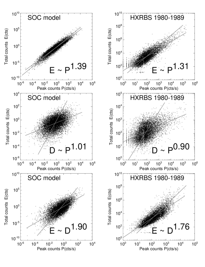
Figure 4.: Scatterplots between the peak count rates $P$, total counts $E$, and flare durations $D$ (left panels) for the same Monte-Carlo simulations of Figure 3, compared with observed values from HXRBS/SMM (1980 – 1989) (right panels). Note the similar scaling laws for the correlations between the parameters.

Based on the random distributions of the values for threshold energies $W_{1}$ (obtained from Equation 15), saturation times $t_{S}$ (Equation 3), and decay times $t_{D}$ (Equation 17), we can then obtain for each parameter combination the peak counts $P$ (with Equation 2),

$$P=W_{0}\left[\exp{\left({t_{S}\over\tau_{G}}\right)}-1\right]\ ,$$

the decay time $D$ (with Equation 6),

$$D=t_{D}\left({P\over W_{0}}\right)\ ,$$

the total flare duration (Equation 8),

$$T=t_{S}+D\ ,$$

and the total counts $E$ (with Equation 10 and Figure 1),

$$E=P\tau_{G}-W_{0}t_{S}+{1\over 2}PD\ ,$$

with the reference value $E_{0}=W_{0}\tau_{G}$.

We perform a Monte-Carlo simulation for a set of $N=11,000$ events, which mimic the distributions of solar flares averaged over a whole solar cycle as observed with HXRBS/SMM during 1980–1989 (Figures 1–3 in Paper I). For each event with randomized sets of values $(t_{S},\tau_{G},t_{D})$ according to the distributions defined in Equations (2), (15), (17) we calculate the parameters $P$, $T$, and $E$ (according to Equations 18, 19, and 20) and show the resulting distributions in Figure 4 (left-hand panels). We obtain a good match with the observed distributions (Figure 4, righ-hand panels, or Figures 1 – 3 in Paper I), with slopes of $\alpha_{P}\approx 1.71\pm 0.04$ (vs. RHESSI: $1.73\pm 0.04$), $\alpha_{E}\approx 1.53\pm 0.03$ (vs. RHESSI: $1.57\pm 0.03$), and $\alpha_{T}\approx 2.24\pm 0.06$ (vs. RHESSI: $2.28\pm 0.06$), for the following model constants: $\tau_{S}=1.0$, $\tau_{G}=1.5$, $\tau_{D}=1.0$, $W_{0}=4$, and $\sigma_{W}=1.5$. Note also that the simulated frequency distributions $N(P),N(E)$, and $N(T)$ all exhibit a roll-over at the lower end of the distributions.

The scatterplots between the three variables $P$, $E$, and $T$ are shown in Figure 4, which also display a comparable scatter as observed in the data, with similar linear regression fits as observed, i.e., $E\propto P^{1.39}$ (vs. RHESSI: $E\propto P^{1.31}$), $D\propto P^{1.01}$ (vs. RHESSI: $D\propto P^{0.90}$), and $E\propto D^{1.90}$ (vs. RHESSI: $E\propto D^{1.76}$).

Thus, we conclude that this model provides more realistic occurrence frequency distributions and parameter correlations than the idealized model with a fixed threshold level $W_{0}$ and decay time $\tau_{D}$.

Figure 5.: Monte-Carlo simulations of a variation of the powerlaw slope of flare peak fluxes by 8% (top), which can be caused by a variation of the growth time $\tau_{G}$ by 38% (bottom left) or by a variation of the mean threshold energy by 26% (bottom right).

4 Discussion and Conclusions

The paramount interpretation of the powerlaw shape of frequency distributions of solar flare parameters is the state of self-organized criticality of a dissipative system (Lu and Hamilton, 1991). This model predicts scale-free distributions of the size parameters of flare events, such as temporal, spatial, and energy parameters. We measured durations, peak values, and time-integrated values of hard X-ray photon counts, which serve as a good proxy of the flare duration, peak energy release rate, and total released flare energies, based on the thick-target bremsstrahlung flare model (Brown, 1971) and the correlations found between these parameters (Crosby et al. 1993). The detailed functional shape of the resulting frequency distributions and the scatterplots of the correlated parameters have been modeled with cellular automaton models before (e.g. Lu and Hamilton etal 1991).

A basic model based on multiplicative nonlinear processes (with exponential growth), random saturation times, and linear decay (Section 2) predicts an exact powerlaw function at the upper end of all frequency distributions, with a rollover at the lower end (Figure 2). However, the predicted relationships between the powerlaw slopes, $\alpha_{P}=\alpha_{T}$ and $\alpha_{E}=(\alpha_{P}+1)/2$, do not agree with the observations (i.e. , $\lower 1.72218pt\hbox{$\;\buildrel<\over{\scriptstyle\sim}\;$}20\%$) within the accuracy of the measured powerlaw slopes ($\lower 1.72218pt\hbox{$\;\buildrel<\over{\scriptstyle\sim}\;$}5\%$). Also the predicted correlation between the parameters does not allow for any scatter, in strong contrast to the observed datapoints.

We develop a more realistic SOC model with randomized parameters (of the threshold levels, saturation times, and decay times), which is able to reproduce closely the powerlaw slopes of the observed frequency distributions and the scatter between correlated parameters. This randomized exponential-growth SOC model predicts different relationships between the powerlaw slopes than the idealized one, which cannot be calculated analytically without approximations, but can easily be generated with numerical (Monte-Carlo) simulations.

In Paper I we discovered a systematic modulation of the powerlaw slope of the frequency distributions of solar flares during three solar cycles, which implies also a modulation of the physical conditions in solar flare sites. A possible coupling could occur between the solar dynamo and the magnetic complexity in the solar photosphere, chromosphere, and corona that leads to magnetic instabilities resulting into flares. The detailed relationship between magnetic complexity and multiplicative chain reactions that occur in a SOC system depends on specific physical models such as magnetic reconnection scenarios. In terms of our analytical SOC model, the powerlaw slope of flare frequency distributions can be modulated by the ratio of growth to saturation times ($\alpha_{P}=1+\tau_{G}/\tau_{S}$; Eq. 5), which can be driven by longer growth times $\tau_{G}$ in magnetically more complex regions during high solar activity periods. A Monte-Carlo simulation shows that a variation of the mean instability growth time by 38% is required to induce a modulation of the powerlaw slope by 8% (Figure 5 left), as observed during the last three solar cycles (Paper I). A shorter growth rate corresponds to faster nonlinear evolution, which could occur in reconnection regions with higher magnetic stress. Alternatively, the mean threshold energy $W_{1}$ could be larger in magnetically unstable regions during high solar activity periods. A Monte-Carlo simulation shows that a change of the mean threshold energy by 26% can explain the observed powerlaw slope variation of 8% (Figure 5 top). A higher threshold could be obtained by stronger magnetic stressing during the solar cycle maximum. Thus, detailed forward-fitting of our analytical SOC model to the observed distributions in various active regions and in specific time intervals of the solar cycle could diagnose the physical conditions of magnetic configurations, which provides important information for statistical flare forecasting.

We thank the referee Brian Dennis for constructive and helpful comments. This work is partially supported by NASA contract NAS5–98033 of the RHESSI mission through the University of California, Berkeley (subcontract SA2241–26308PG) and NASA grant NNX08AJ18G. We acknowledge access to solar mission data and flare catalogs from the Solar Data Analysis Center (SDAC) at the NASA Goddard Space Flight Center (GSFC).

References

Aschwanden, M.J., Dennis, B.R., Benz, A.O. 1998, Logistic avalanche processes, elementary time structures, and frequency distributions of flares, Astrophys. J. 497, 972-993.

Aschwanden, M.J., 2010a, The State of Self-Organized Criticality of the Sun During the Last Three Solar Cycles. I. Observations, Solar Physics, (this volume), subm. (Paper I).

Aschwanden, M.J., 2010b, Self-Organized Criticality in Astrophysics. The Statistics of Nonlinear Processes in the Universe, Springer-Praxis: Heidelberg, New York (in press).

Bak, P., Tang, C., Wiesenfeld, K. 1987, Self-organized criticality: An explanation of 1/f noise, Phys. Rev. Lett. 59/4, 381-384.

Brown, J.C. 1971, The deduction of energy spectra of non-thermal electrons in flares from the observed dynamic spectra of Hard X-Ray bursts, Solar Phys. 18, 489-502.

Charbonneau, P., McIntosh, S.W., Liu, H.L., and Bogdan, T.J. 2001, Avalanche models for solar flares, Solar Phys., 203, 321-353.

Crosby, N.B., Aschwanden, M.J., Dennis, B.R. 1993, Frequency distributions and correlations of solar X-ray flare parameters, Solar Phys. 143, 275-299.

Crosby, N.B. 1996, Contribution à l’Etude des Phénomènes Eruptifs du Soleil en Rayons Z à partir des Observations de l’Expérience WATCH sur le Satellite GRANAT, PhD Thesis, University Paris VII, Meudon, Paris.

Fermi, E. 1949, On the origin of the cosmic radiation, Phys. Rev. Lett. 75, 1169.

Georgoulis, M.K., Vilmer,N., Crosby,N.B. 2001, A Comparison Between Statistical Properties of Solar X-Ray Flares and Avalanche Predictions in Cellular Automata Statistical Flare Models, Astron. Astrophys. 367, 326-338.

Huberman, B.A. and Adamic, L. 1999, Growth dynamics of the World-Wide Web, Nature 401, 131.

Lu, E.T. and Hamilton, R.J. 1991, Avalanches and the distribution of solar flares, Astrophys. J., 380, L89-L92.

Lu, E.T. 1995, Constraints on energy storage and release models for astrophysical transients and solar flares, Astrophys. J., 447, 416-418.

Rosner, R. and Vaiana, G.S. 1978, Cosmic flare transients: constraints upon models for energy storage and release derived from the event frequency distribution, Astrophys. J. 222, 1104-1108.

Simkin, M.V., and Roychowdhury, V.P. 2006, Re-inventing Willis, eprint arXiv:physics 0601192.

Wheatland, M.S. 2000, Do solar flares exhibit an interval-size relationship? Solar Phys., 191, 381-389.

Willis, J.C. and Yule, G.U. 1922, Some statistics of evolution and geographical distribution in plants and animals, and their significance, Nature, 109, 177-179.