HAT-P-26b: A Low-Density Neptune-Mass Planet Transiting a K Star

Abstract

We report the discovery of HAT-P-26b, a transiting extrasolar planet orbiting the moderately bright V=11.744 K1 dwarf star GSC 0320-01027, with a period $P=4.234516\pm 0.000015$ d, transit epoch $T_{c}=2455304.65122\pm 0.00035$ (BJD), and transit duration $0.1023\pm 0.0010$ d. The host star has a mass of $0.82\pm 0.03$ $M_{\sun}$, radius of $0.79_{-0.04}^{+0.10}$ $R_{\sun}$, effective temperature $5079\pm 88$ K, and metallicity $\rm[Fe/H]=-0.04\pm 0.08$. The planetary companion has a mass of $0.059\pm 0.007$ $M_{\rm J}$, and radius of $0.565_{-0.032}^{+0.072}$ $R_{\rm J}$ yielding a mean density of $0.40\pm 0.10$ $\rm g\,cm^{-3}$. HAT-P-26b is the fourth Neptune-mass transiting planet discovered to date. It has a mass that is comparable to those of Neptune and Uranus, and slightly smaller than those of the other transiting Super-Neptunes, but a radius that is $\sim$65% larger than those of Neptune and Uranus, and also larger than those of the other transiting Super-Neptunes. HAT-P-26b is consistent with theoretical models of an irradiated Neptune-mass planet with a 10 $M_{\earth}$ heavy element core that comprises $\gtrsim 50\%$ of its mass with the remainder contained in a significant hydrogen-helium envelope, though the exact composition is uncertain as there are significant differences between various theoretical models at the Neptune-mass regime. The equatorial declination of the star makes it easily accessible to both Northern and Southern ground-based facilities for follow-up observations.

1. Introduction

Transiting exoplanets (TEPs) are tremendously useful objects for studying the properties of planets outside of the solar system because their photometric transits, combined with precise measurements of the radial velocity variations of their host stars, enable determinations of their masses and radii. Of the $\gtrsim 90$ confirmed TEPs discovered to date, all but five are Saturn or Jupiter-size gas giant planets with masses above $0.1$ $M_{\rm J}$. The five TEPs below this limit, including the Super-Earths CoRoT-7b ($M=0.015\pm 0.003$ $M_{\rm J}$, $R=0.15\pm 0.008$ $R_{\rm J}$; Léger et al., 2009; Queloz et al., 2009), and GJ 1214b ($M=0.0206\pm 0.0031$ $M_{\rm J}$, $R=0.239\pm 0.012$ $R_{\rm J}$; Charbonneau et al., 2009), and the Super-Neptunes GJ 436b ($M=0.078\pm 0.006$ $M_{\rm J}$, $R=0.376\pm 0.022$ $R_{\rm J}$; Butler et al., 2004; Gillon et al., 2007; Southworth, 2009), HAT-P-11b ($M=0.081\pm 0.009$ $M_{\rm J}$, $R=0.422\pm 0.014$ $R_{\rm J}$; Bakos et al., 2010), and Kepler-4b ($M=0.081\pm 0.014$ $M_{\rm J}$, $R=0.515^{+0.2}_{-0.098}$ $R_{\rm J}$; Borucki et al., 2010; Kipping & Bakos, 2010a) are likely composed primarily of elements heavier than hydrogren and helium, and are therefore assumed to be qualitatively different from the more massive gas giants. In addition to these five TEPs, the candidate TEP Kepler-9d has an estimated radius of $1.4$ $R_{\earth}$ (Holman et al., 2010), and is most likely a low-mass planet (Torres et al., 2010), but currently lacks a mass determination.

While the gas giant planets exhibit a wide range of radii at fixed mass (and hence a great diversity in their physical structure at fixed mass), the low mass TEPs, together with the six Solar System planets smaller than Saturn, appear to follow a nearly monotonic relation between mass and radius. The two Super-Neptunes with precise radius measurements (GJ 436b and HAT-P-11b) have radii that are similar to one another (to within 15%) as well as to Uranus ($M=0.0457$ $M_{\rm J}$, $R=0.358$ $R_{\rm J}$) and Neptune ($M=0.0540$ $M_{\rm J}$, $R=0.346$ $R_{\rm J}$). While the mass and radius of Kepler-4b given in the discovery paper (Borucki et al., 2010) are similar to those of GJ 436b and HAT-P-11b, a reanalysis by Kipping & Bakos (2010a) finds that the radius may be $\sim 40$% larger, though with a $20\%$ uncertainty, it may still be similar to the other Super-Neptunes. The lack of significant scatter in the radii among Uranus, Neptune, and the Super-Neptunes is perhaps surprising given the vast range of radii permitted by theoretical structure models for planets in this mass range. For example, the theoretical models by Fortney et al. (2007) predict that a $1~{}{\rm Gyr}$ nonirradiated Neptune-mass planet may have a radius that ranges from 0.14 $R_{\rm J}$ (pure iron composition) to 0.29 $R_{\rm J}$ (pure water ice composition) or 0.86 $R_{\rm J}$ (pure gas composition). These same models also predict that the radii of gas-dominated Neptune-mass planets should be far more sensitive to stellar irradiation than those of Jupiter-mass planets. For example, a $1~{}{\rm Gyr}$ pure hydrogen-helium Neptune-mass planet at $0.045$ AU has a radius of $1.49$ $R_{\rm J}$ compared to $1.16$ $R_{\rm J}$ for a similarly irradiated Jupiter-mass planet.

In this paper we present the discovery of HAT-P-26b, a TEP orbiting the relatively bright star GSC 0320-01027 with a mass similar to that of Neptune, but with a radius of $0.57$ $R_{\rm J}$ or 65% larger than that of Neptune. This is the 26th TEP discovered by the Hungarian-made Automated Telescope Network (HATNet; Bakos et al., 2004) survey. In operation since 2003, HATNet has now covered approximately 14% of the sky, searching for TEPs around bright stars ($8\lesssim r\lesssim 14.5$). HATNet operates six wide-field instruments: four at the Fred Lawrence Whipple Observatory (FLWO) in Arizona, and two on the roof of the hangar servicing the Smithsonian Astrophysical Observatory’s Submillimeter Array, in Hawaii.

The layout of the paper is as follows. In Section 2 we report the detection of the photometric signal and the follow-up spectroscopic and photometric observations of HAT-P-26. In Section 3 we describe the analysis of the data, beginning with the determination of the stellar parameters, continuing with a discussion of the methods used to rule out nonplanetary, false positive scenarios which could mimic the photometric and spectroscopic observations, and finishing with a description of our global modeling of the photometry and radial velocities. Our findings are discussed in Section 4.

2. Observations

2.1. Photometric detection

The transits of HAT-P-26b were detected with the HAT-5 and HAT-6 telescopes in Arizona, and with the HAT-8 and HAT-9 telescopes in Hawaii. Two regions around GSC 0320-01027, corresponding to fields internally labeled as 376 and 377, were both observed on a nightly basis between 2009 Jan and 2009 Aug, whenever weather conditions permitted. For field 376 we gathered 11,500 exposures of 5 minutes at a 5.5 minute cadence. Approximately 1500 of these exposures were rejected by our photometric pipeline because they yielded poor photometry for a significant number of stars. Each image contained approximately 17,000 stars down to Sloan $r\sim 14.5$. For the brightest stars in the field, we achieved a per-image photometric precision of 4 mmag. For field 377 we gathered 5200 exposures with the same exposure time and cadence; we rejected aproximately 700 exposures. Each image contained approximately 19,000 stars down to Sloan $r\sim 14.5$. We achieved a similar photometric precision for the brightest stars in this field.

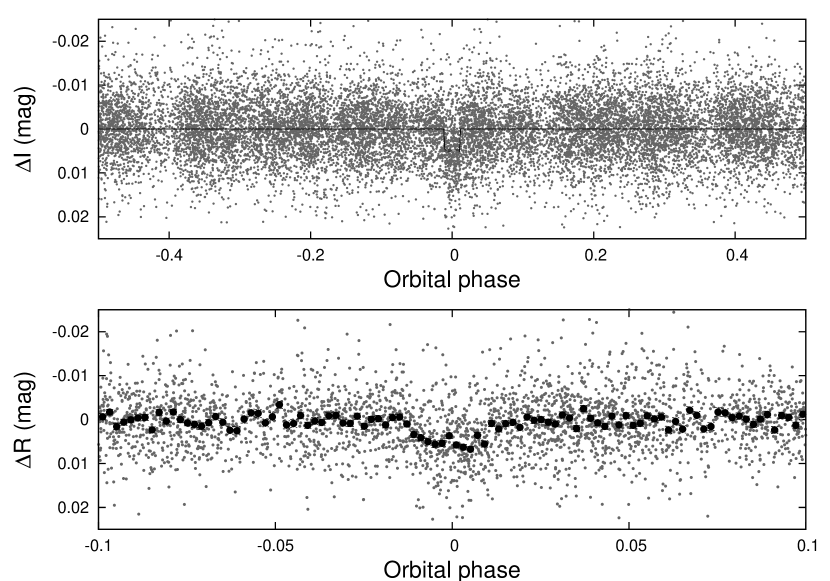
Figure 1.— Unbinned light curve of HAT-P-26 including all 14,500 instrumental Sloan $r$ band 5.5 minute cadence measurements obtained with the HAT-5, HAT-6, HAT-8 and HAT-9 telescopes of HATNet (see the text for details), and folded with the period $P=4.2345156$ days resulting from the global fit described in Section 3). The solid line shows the “P1P3” transit model fit to the light curve (Section 3.3). The lower panel shows a zoomed-in view of the transit; the dark filled points show the light curve binned in phase using a bin-size of 0.002.

The calibration of the HATNet frames was carried out using standard photometric procedures. The calibrated images were then subjected to star detection and astrometry, as described in Pál & Bakos (2006). Aperture photometry was performed on each image at the stellar centroids derived from the Two Micron All Sky Survey (2MASS; Skrutskie et al., 2006) catalog and the individual astrometric solutions. The resulting light curves were decorrelated (cleaned of trends) using the External Parameter Decorrelation (EPD; see Bakos et al., 2010) technique in “constant” mode and the Trend Filtering Algorithm (TFA; see Kovács et al., 2005). The light curves were searched for periodic box-shaped signals using the Box Least-Squares (BLS; see Kovács et al., 2002) method. We detected a significant signal in the light curve of GSC 0320-01027 (also known as 2MASS 14123753+0403359; $\alpha=14^{\mathrm{h}}12^{\mathrm{m}}37.44{\mathrm{s}}$, $\delta=+04{\arcdeg}03{\arcmin}36.0{\arcsec}$; J2000; V=11.744 Droege et al., 2006), with an apparent depth of $\sim 4.9$ mmag ($\sim 5.5$ mmag when using TFA in signal-reconstruction mode), and a period of $P=4.2345$ days (see Figure 1). The drop in brightness had a first-to-last-contact duration, relative to the total period, of $q=0.0242\pm 0.0002$, corresponding to a total duration of $Pq=2.455\pm 0.025$ hr.

We removed the transits from the combined 376/377 light curve and searched for additional transiting objects using the BLS method; no significant signals were found in the data. We also searched the transit-cleaned light curve for periodic variations (e.g. due to stellar rotation) using the Discrete Fourier Transform (e.g. Kurtz, 1985), and found no coherent variation with an amplitude greater than $0.4$ mmag.

2.2. Reconnaissance Spectroscopy

As is routine in the HATNet project, all candidates are subjected to careful scrutiny before investing valuable time on large telescopes. This includes spectroscopic observations at relatively modest facilities to establish whether the transit-like feature in the light curve of a candidate might be due to astrophysical phenomena other than a planet transiting a star. Many of these false positives are associated with large radial-velocity variations in the star (tens of $\rm km\,s^{-1}$) that are easily recognized.

To carry out this reconnaissance spectroscopy, we made use of the Tillinghast Reflector Echelle Spectrograph (TRES; Fűrész, 2008) on the 1.5 m Tillinghast Reflector at FLWO. This instrument provides high-resolution spectra which, with even modest signal-to-noise (S/N) ratios, are suitable for deriving RVs with moderate precision ($\lesssim 0.3$ $\rm km\,s^{-1}$) for slowly rotating stars. We also use these spectra to estimate effective temperatures, surface gravities, and projected rotational velocities of the target star. Using the medium fiber on TRES, we obtained two spectra of HAT-P-26 on the nights of 2009 Dec 26 and 2009 Dec 27. The spectra have a resolution of $\lambda/\Delta\lambda\approx 44,\!000$ and a wavelength coverage of $\sim$ 3900-8900 Å. The spectra were extracted and analyzed according to the procedure outlined by Buchhave et al. (2010) and Quinn et al. (2010). The individual velocity measurements of $14.62$ $\rm km\,s^{-1}$ and $14.81$ $\rm km\,s^{-1}$ were consistent with no detectable RV variation within the measurement precision. Both spectra were single-lined, i.e., there is no evidence for additional stars in the system. The atmospheric parameters we infer from these observations are the following: effective temperature $T_{\rm eff\star}=5125\pm 125\,K$, surface gravity $\log{g_{\star}}=4.5\pm 0.5$ (log cgs), and projected rotational velocity $v\sin{i}=1.0\pm 1.0\,\rm km\,s^{-1}$. The effective temperature corresponds to an early K dwarf. The mean heliocentric RV of HAT-P-26 is $\gamma_{\rm RV}=+14.72\pm 0.10$ $\rm km\,s^{-1}$.

2.3. High resolution, high S/N spectroscopy

Given the significant transit detection by HATNet, and the encouraging TRES results that rule out obvious false positives, we proceeded with the follow-up of this candidate by obtaining high-resolution, high-S/N spectra to characterize the RV variations, and to refine the determination of the stellar parameters. For this we used the HIRES instrument (Vogt et al., 1994) on the Keck I telescope located on Mauna Kea, Hawaii, between 2009 Dec and 2010 June. The width of the spectrometer slit was $0\farcs 86$, resulting in a resolving power of $\lambda/\Delta\lambda\approx 55,\!000$, with a wavelength coverage of $\sim$3800–8000 Å.

We obtained 12 exposures through an iodine gas absorption cell, which was used to superimpose a dense forest of $\mathrm{I}_{2}$ lines on the stellar spectrum and establish an accurate wavelength fiducial (see Marcy & Butler, 1992). An additional exposure was taken without the iodine cell, for use as a template in the reductions. Relative RVs in the solar system barycentric frame were derived as described by Butler et al. (1996), incorporating full modeling of the spatial and temporal variations of the instrumental profile. The RV measurements and their uncertainties are listed in Table 1. The period-folded data, along with our best fit described below in Section 3, are displayed in Figure 2.

Figure 2.— Top panel: Keck/HIRES RV measurements for HAT-P-26 shown as a function of orbital phase, along with our best-fit model (see Table 5). Zero phase corresponds to the time of mid-transit. The center-of-mass velocity has been subtracted. Second panel: Velocity $O\!-\!C$ residuals from the best fit. The error bars include a component from astrophysical/instrumental jitter ($1.6$ $\rm m\,s^{-1}$) added in quadrature to the formal errors (see Section 3.3). Third panel: Bisector spans (BS), with the mean value subtracted. The measurement from the template spectrum is included (see Section 3.2). Bottom panel: Chromospheric activity index $S_{\rm HK}$ measured from the Keck spectra. Note the different vertical scales of the panels. Observations shown twice are represented with open symbols.

Figure 3.— Calcium K (left) and H (right) line profile in selected Keck/HIRES observations of HAT-P-26. Both panels show three spectra overlaid; data taken at high, median, and low activity, as characterized by the $S_{\rm HK}$ index. Low-level emission is clearly detected in the cores of both lines. The lack of apparent variation (the three plotted spectra are indistinguishable) indicates the chromospheric stability of this star over the course of our observations. The spectra are matched to a common flux/wavelength scale using points outside the H and K line cores. The vertical axes give the counts in units of CCD $e^{-}$ per wavelength bin for the reference spectrum.

In the same figure we show also the $S_{\rm HK}$ index, which is a measure of the chromospheric activity of the star derived from the flux in the cores of the Ca II H and K lines (Figure 3 shows representative Keck spectra including the H and K lines for HAT-P-26). This index was computed and calibrated to the scale of Vaughan, Preston & Wilson (1978) following the procedure described by Isaacson & Fischer (2010). We find a median value of $S_{\rm HK}=0.182$ with a standard deviation of $0.004$. Assuming $B-V=0.89$ based on the effective temperature measured in Section 3.1, this corresponds to $\log R^{\prime}_{\rm HK}=-4.992$ (Noyes et al., 1984). From Isaacson & Fischer (2010) the lower tenth percentile $S_{\rm HK}$ value among California Planet Search (CPS) targets with $B-V=0.89$ is $0.168$. The measured $S_{\rm HK}$ value is only slightly higher than this, implying that HAT-P-26 is a chromospherically quiet star. We do not detect any significant variation of the $S_{\rm HK}$ index correlated with orbital phase; such a correlation might have indicated that the RV variations could be due to stellar activity, casting doubt on the planetary nature of the candidate.

Table 1 Relative radial velocities, bisector spans, and activity index measurements of HAT-P-26.

BJD	RV	$\sigma_{\rm RV}$	BS	$\sigma_{\rm BS}$	$S_{\rm HK}$	Phase
(2,454,000$+$)	($\rm m\,s^{-1}$)	($\rm m\,s^{-1}$)	($\rm m\,s^{-1}$)	($\rm m\,s^{-1}$)
$1193.11925$	$6.67$	$1.87$	$3.71$	$2.51$	$0.1870$	$0.661$
$1193.12855$	$\cdots$	$\cdots$	$4.74$	$3.90$	$0.1830$	$0.663$
$1194.16006$	$10.75$	$1.62$	$-1.85$	$3.76$	$0.1850$	$0.907$
$1252.02017$	$2.23$	$1.89$	$8.33$	$3.95$	$0.1890$	$0.571$
$1285.14629$	$-7.14$	$2.58$	$-24.47$	$4.35$	$0.1760$	$0.394$
$1320.84584$	$8.96$	$2.00$	$-13.90$	$5.02$	$0.1840$	$0.824$
$1343.78649$	$-3.54$	$1.79$	$-8.59$	$3.23$	$0.1870$	$0.242$
$1350.92272$	$4.54$	$2.18$	$-14.55$	$4.65$	$0.1740$	$0.927$
$1351.91410$	$-6.17$	$1.70$	$7.80$	$4.04$	$0.1800$	$0.161$
$1372.77275$	$-6.44$	$1.65$	$4.63$	$2.63$	$0.1800$	$0.087$
$1373.75770$	$-9.14$	$1.71$	$5.32$	$4.79$	$0.1810$	$0.320$
$1374.91646$	$2.06$	$1.78$	$22.23$	$4.36$	$0.1780$	$0.593$
$1375.80851$	$6.63$	$1.71$	$6.59$	$3.90$	$0.1820$	$0.804$

Note. — For the iodine-free template exposures there is no RV measurement, but the BS and $S_{\rm HK}$ index can still be determined.

2.4. Photometric follow-up observations

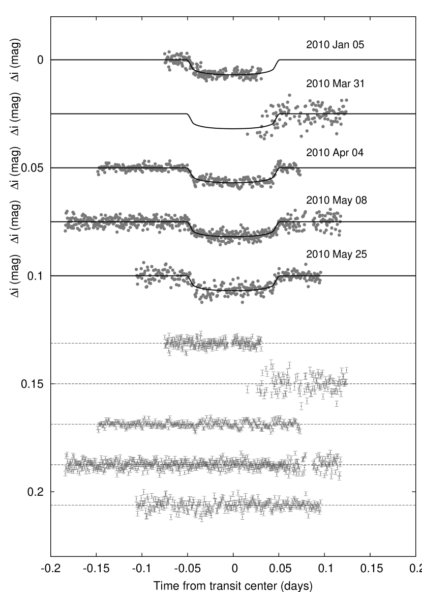
Figure 4.— Unbinned instrumental Sloan $i$ band light curves, acquired with KeplerCam at the FLWO 1.2 m telescope. The light curves have been EPD- and TFA-processed, as described in § 3.3. The dates of the events are indicated. Curves after the first are displaced vertically for clarity. Our best fit from the global modeling described in Section 3.3 is shown by the solid lines. Residuals from the fits are displayed at the bottom, in the same order as the top curves. The error bars represent the photon and background shot noise, plus the readout noise.

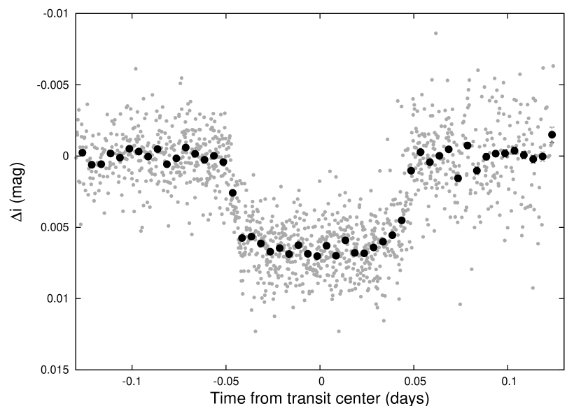
Figure 5.— The combined Sloan $i$ band KeplerCam light curve of HAT-P-26 folded with the period $P=4.2345156$ days resulting from the global fit described in Section 3. The dark filled circles show the light curve binned in folded time with a bin-size of 0.005 days. The median uncertainty on the binned points is $0.19$ mmag.

In order to permit a more accurate modeling of the light curve, we conducted additional photometric observations with the KeplerCam CCD camera on the FLWO 1.2 m telescope. We observed five transit events of HAT-P-26 on the nights of 2010 Jan 05, Mar 31, Apr 04, May 08 and May 25 (Figure 4). These observations are summarized in Table 2.

Table 2 Summary of photometric follow-up observations

Facility	Date	Number of Images	Median Cadence (s)	Filter
KeplerCam/FLWO 1.2 m	2010 Jan 05	191	40	Sloan $i$ band
KeplerCam/FLWO 1.2 m	2010 Mar 31	161	59	Sloan $i$ band
KeplerCam/FLWO 1.2 m	2010 Apr 04	291	64	Sloan $i$ band
KeplerCam/FLWO 1.2 m	2010 May 08	596	44	Sloan $i$ band
KeplerCam/FLWO 1.2 m	2010 May 25	298	59	Sloan $i$ band

The reduction of these images, including basic calibration, astrometry, and aperture photometry, was performed as described by Bakos et al. (2010). We performed EPD and TFA to remove trends simultaneously with the light curve modeling (for more details, see Section 3, and Bakos et al. 2010). The final time series are shown in the top portion of Figure 4, along with our best-fit transit light curve model described below; the individual measurements are reported in Table 3. The combined phase-folded follow-up light curve is displayed in Figure 5.

Table 3High-precision differential photometry of HAT-P-26

BJD	Mag	$\sigma_{\rm Mag}$	Mag(orig)	Filter
(2,400,000$+$)
$55202.94802$	$-0.00279$	$0.00105$	$10.17790$	$i$
$55202.94847$	$0.00137$	$0.00106$	$10.18150$	$i$
$55202.94909$	$0.00132$	$0.00106$	$10.18130$	$i$
$55202.94954$	$0.00079$	$0.00106$	$10.18110$	$i$
$55202.95018$	$-0.00047$	$0.00105$	$10.17920$	$i$
$55202.95063$	$-0.00029$	$0.00106$	$10.17980$	$i$
$55202.95126$	$-0.00131$	$0.00106$	$10.17960$	$i$
$55202.95171$	$-0.00097$	$0.00105$	$10.17950$	$i$
$55202.95237$	$0.00334$	$0.00107$	$10.18530$	$i$
$55202.95282$	$-0.00366$	$0.00106$	$10.17800$	$i$

Note. — This table is available in a machine-readable form in the online journal. A portion is shown here for guidance regarding its form and content.

3. Analysis

3.1. Properties of the parent star

Fundamental parameters of the host star HAT-P-26 such as the mass ($M_{\star}$) and radius ($R_{\star}$), which are needed to infer the planetary properties, depend strongly on other stellar quantities that can be derived spectroscopically. For this we have relied on our template spectrum obtained with the Keck/HIRES instrument, and the analysis package known as Spectroscopy Made Easy (SME; Valenti & Piskunov, 1996), along with the atomic line database of Valenti & Fischer (2005). SME yielded the following values and uncertainties: effective temperature $T_{\rm eff\star}=5079\pm 88$ K, stellar surface gravity $\log{g_{\star}}=4.53\pm 0.06$ (cgs), metallicity $\rm[Fe/H]=-0.04\pm 0.08$ dex, and projected rotational velocity $v\sin{i}=1.8\pm 0.5\,\rm km\,s^{-1}$, in which the uncertainties for $T_{\rm eff\star}$ and $\rm[Fe/H]$ have been increased by a factor of two over their formal values to include our estimates of the systematic uncertainties.

In principle the effective temperature and metallicity, along with the surface gravity taken as a luminosity indicator, could be used as constraints to infer the stellar mass and radius by comparison with stellar evolution models. However, the effect of $\log{g_{\star}}$ on the spectral line shapes is quite subtle, and as a result it is typically difficult to determine accurately, so that it is a rather poor luminosity indicator in practice. For planetary transits a stronger constraint is often provided by $\rho_{\star}$ the mean stellar density, which is closely related to the $a/R_{\star}$ normalized semimajor axis. The quantity $\rho_{\star}$ can be derived directly from the combination of the transit light curves (Seager & Mallén-Ornelas, 2003; Sozzetti et al., 2007) and the RV data (required for eccentric cases, see Section 3.3). This, in turn, allows us to improve on the determination of the spectroscopic parameters by supplying an indirect constraint on the weakly determined spectroscopic value of $\log{g_{\star}}$ that removes degeneracies. We take this approach here, as described below. The validity of our assumption, namely that the adequate physical model describing our data is a planetary transit (as opposed to a blend), is shown later in Section 3.2.

Our values of $T_{\rm eff\star}$, $\log{g_{\star}}$, and $\rm[Fe/H]$ were used to determine auxiliary quantities needed in the global modeling of the follow-up photometry and radial velocities (specifically, the limb-darkening coefficients). This modeling, the details of which are described in Section 3.3, uses a Monte Carlo approach to deliver the numerical probability distribution of $\rho_{\star}$ and other fitted variables. For further details we refer the reader to Pál (2009b). When combining $\rho_{\star}$ (a luminosity proxy) with assumed Gaussian distributions for $T_{\rm eff\star}$ and $\rm[Fe/H]$ based on the SME determinations, a comparison with stellar evolution models allows the probability distributions of other stellar properties to be inferred, including $\log{g_{\star}}$. Here we use the stellar evolution calculations from the Yonsei-Yale (YY) series by Yi et al. (2001).

For the case of HAT-P-26b, the eccentricity is poorly constrained by the RV data due to the low semiamplitude of the signal. This in turn leads to a significant uncertainty on $\rho_{\star}$. However, not all combinations of $\rm[Fe/H]$, $T_{\rm eff\star}$ and $\rho_{\star}$ are realized by physical stellar models. In particular, if we conservatively adopt a maximum stellar age of $13.8$ Gyr, corresponding approximately to the age of the universe (Komatsu et al., 2010, find $13.75\pm 0.11$ Gyr), and a minimum age of $100$ Myr, corresponding roughly to the zero-age main-sequence, stars with $T_{\rm eff\star}=5079$ and $\rm[Fe/H]=-0.04$ are not found to have densities in the range $0.24\,\rm g\,cm^{-3}<\rho_{\star}<2.06\,\rm g\,cm^{-3}$ or surface gravities in the range $3.915<\log{g_{\star}}<4.514$ (here $0.24\,\rm g\,cm^{-3}$ corresponds to an evolved star with $M=0.94$ $M_{\sun}$, while $2.06\,\rm g\,cm^{-3}$ corresponds to a main sequence star with $M=0.79$ $M_{\sun}$). Figure 6 shows the inferred location of the star in a diagram of $\rho_{\star}$ versus $T_{\rm eff\star}$, analoguous to the classical H-R diagram, for three cases: fixing the eccentricity of the orbit to zero, allowing the eccentricity to vary, and allowing the eccentricity to vary, but only accepting parameter combinations which match to a position in the YY isochrones with $0.1\,{\rm Gyr}<{\rm age}<13.8\,{\rm Gyr}$. The stellar properties and their approximate 1$\sigma$ and 2$\sigma$ confidence boundaries are displayed against the backdrop of Yi et al. (2001) isochrones for the measured metallicity of $\rm[Fe/H]$ = $-0.04$, and a range of ages. For the zero eccentricity case the comparison against the model isochrones was carried out for each of 30,000 Monte Carlo trial sets (see Section 3.3). We find good overlap between the trials and the model isochrones–in 71% of the trials, the $\rm[Fe/H]$, $T_{\rm eff\star}$ and $\rho_{\star}$ parameter combination matched to a physical location in the H-R diagram that has an age that is within the aforementioned range. However, when the eccentricity is allowed to vary, the model for the light curves and RV data tends toward low values of $\rho_{\star}$ which may only be fit by pre-main sequence stellar models, or stellar models older than the age of the universe. In this case only 15% out of 100,000 Monte Carlo trial sets match to physical locations in the H-R diagram with ages within the allowed range. By requiring the star to have an age between 0.1 Gyr and 13.8 Gyr, we effectively impose a tighter constraint on the orbital eccentricity than is possible from the RV data alone (we find an eccentricity of $e=0.124\pm 0.060$, as compared with $e=0.24\pm 0.12$ when not requiring a match to the stellar models; see also Section 3.3).

Adopting the parameters which result from allowing the eccentricity to vary while requiring the star to have an age between 0.1 Gyr and 13.8 Gyr yields a stellar surface gravity of $\log{g_{\star}}=4.56\pm 0.06$, which is very close to the value from our SME analysis. The values for the atmospheric parameters of the star are collected in Table 4, together with the adopted values for the macroturbulent and microturbulent velocities.

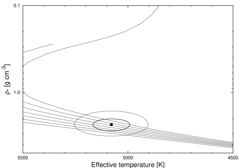
Figure 6.— Model isochrones from Yi et al. (2001) for the measured metallicity of HAT-P-26, $\rm[Fe/H]$= $-0.04$, and ages in 2 Gyr increments between 1 and 13 Gyr (left to right). Note that a logarithmic scale is used for the vertical axis. The measured values of $T_{\rm eff\star}$ and $\rho_{\star}$ are shown together with their approximate $1\sigma$ and $2\sigma$ confidence boundaries for models where the eccentricity is fixed to 0 (top), the eccentricity is allowed to vary (bottom), and the eccentricity is allowed to vary, but only models which match to an isochrone with an age between 0.1 Gyr and 13.8 Gyr are accepted (bottom). We adopt the parameters shown in the bottom panel.

The stellar evolution modeling provides color indices that may be compared against the measured values as a sanity check. The best available measurements are the near-infrared magnitudes from the 2MASS Catalogue (Skrutskie et al., 2006), $J_{\rm 2MASS}=10.080\pm 0.022$, $H_{\rm 2MASS}=9.685\pm 0.023$ and $K_{\rm 2MASS}=9.581\pm 0.023$; which we have converted to the photometric system of the models (ESO) using the transformations by Carpenter (2001). The resulting measured color index is $J-K=0.530\pm 0.035$. This is within 1$\sigma$ of the predicted value from the isochrones of $J-K=0.55\pm 0.02$. The distance to the object may be computed from the absolute $K$ magnitude from the models ($M_{\rm K}=3.98\pm 0.19$) and the 2MASS $K_{s}$ magnitude, which has the advantage of being less affected by extinction than optical magnitudes. The result is $134_{-8}^{+18}$ pc, where the uncertainty excludes possible systematics in the model isochrones that are difficult to quantify.

An additional check on our stellar model can be performed by comparing the isochrone-based age estimate to activity-based age estimates. Using the activity-rotation and activity-age relations from Mamajek & Hillenbrand (2008, equations 5 and 3) we convert the value of $\log R^{\prime}_{\rm HK}$ determined in Section 2.3 into a Rossby number ($R_{O}=P_{\rm rot}/\tau_{c}$, where $P_{\rm rot}$ is the rotation period and $\tau_{c}$ is the convective turnover time-scale) and an age. We find $R_{O}=2.2\pm 0.2$, and $\log(\tau)=9.80\pm 0.15$ or $\tau=6.4^{+2.7}_{-1.9}$ Gyr, where we adopt the estimated uncertainties on $R_{O}$ and $\log(\tau)$ from Mamajek & Hillenbrand (2008). The $R_{O}$ value may be converted to a rotation period using the relation for $\tau_{c}$ given by Noyes et al. (1984). We find $P_{\rm rot}=48\pm 4$ d. The rotation period and color may also be used to obtain a separate age estimate from the gyrochronology relation given by Mamajek & Hillenbrand (2008, equation 12). This gives $\tau=7.8^{+1.4}_{-1.2}$ Gyr, where the scatter on this relation is less than the scatter on the age-activity relation because it includes a correction for stellar color. The age inferred from $\log R^{\prime}_{\rm HK}$ is consistent with the isochrone-based age of $9.0_{-4.9}^{+3.0}$ Gyr. The equatorial rotation period inferred from the spectroscopic determination of $v\sin i$ assuming $\sin i=1$ is $P_{\rm rot,v\sin i}=22.3^{+17.2}_{-4.6}$ d, which is shorter than the expected value based on $\log R^{\prime}_{\rm HK}$, though the upper limit is poorly constrained.

As discussed below in Section 3.3 we measure a RV jitter of $1.6$ $\rm m\,s^{-1}$ for HAT-P-26. From Isaacson & Fischer (2010) the lower tenth percentile jitter among HIRES/Keck observations for CPS stars with $0.7<B-V<1.0$ and $S_{\rm HK}=0.182$ is $2.17$ $\rm m\,s^{-1}$, implying that HAT-P-26 has an exceptionally low jitter value–only a handful of stars in this color range have measured jitter values less than that of HAT-P-26. We note that the jitter may be higher ($2.4$ $\rm m\,s^{-1}$) if the orbit is circular, though this value is still quite low.

Table 4 Stellar parameters for HAT-P-26

Parameter	Value	Source
Spectroscopic properties
$T_{\rm eff\star}$ (K)	$5079\pm 88$	SME
$\rm[Fe/H]$	$-0.04\pm 0.08$	SME
$v\sin{i}$ ($\rm km\,s^{-1}$)	$1.8\pm 0.5$	SME
$v_{\rm mac}$ ($\rm km\,s^{-1}$)	$2.95$	SME
$v_{\rm mic}$ ($\rm km\,s^{-1}$)	$0.85$	SME
$\gamma_{\rm RV}$ ($\rm km\,s^{-1}$)	$+14.72\pm 0.10$	TRES
Photometric properties
$V$ (mag)	11.744	TASS
$V\!-\!I_{C}$ (mag)	$0.96\pm 0.11$	TASS
$J$ (mag)	$10.080\pm 0.022$	2MASS
$H$ (mag)	$9.685\pm 0.023$	2MASS
$K_{s}$ (mag)	$9.581\pm 0.023$	2MASS
Derived properties
$M_{\star}$ ($M_{\sun}$)	$0.816\pm 0.033$	YY+$a/R_{\star}$+SME
$R_{\star}$ ($R_{\sun}$)	$0.788_{-0.043}^{+0.098}$	YY+$a/R_{\star}$+SME
$\log{g_{\star}}$ (cgs)	$4.56\pm 0.06$	YY+$a/R_{\star}$+SME
$L_{\star}$ ($L_{\sun}$)	$0.38_{-0.06}^{+0.16}$	YY+$a/R_{\star}$+SME
$M_{V}$ (mag)	$6.03\pm 0.24$	YY+$a/R_{\star}$+SME
$M_{K}$ (mag,ESO)	$3.98\pm 0.19$	YY+$a/R_{\star}$+SME
Age (Gyr)	$9.0_{-4.9}^{+3.0}$	YY+$a/R_{\star}$+SME
Distance (pc)	$134_{-8}^{+18}$	YY+$a/R_{\star}$+SME

3.2. Excluding blend scenarios

Our initial spectroscopic analyses discussed in Section 2.2 and Section 2.3 rule out the most obvious astrophysical false positive scenarios. However, more subtle phenomena such as blends (contamination by an unresolved eclipsing binary, whether in the background or associated with the target) can still mimic both the photometric and spectroscopic signatures we see. In the following sections we consider and rule out the possibility that such scenarios may have caused the observed photometric and spectroscopic features.

3.2.1 Spectral line-bisector analysis

Following Queloz et al. (2001); Torres et al. (2007), we explored the possibility that the measured radial velocities are not real, but are instead caused by distortions in the spectral line profiles due to contamination from a nearby unresolved eclipsing binary. A bisector analysis based on the Keck spectra was done as described in §5 of Bakos et al. (2007). While the bisector spans show no evidence for variation in phase with the orbital period, the scatter on these values ($13.3$ $\rm m\,s^{-1}$ RMS) is large relative to the RV semi-amplitude ($\sim 8$ $\rm m\,s^{-1}$), and thus the lack of variation does not provide a strong constraint on possible blend scenarios. We note that some of the scatter in the bisector spans may be due to contamination from the sky background (predominately moonlight)–correcting the bisector spans for sky contamination as discussed by Hartman et al. (2010) reduces the RMS to $\sim 10.0$ $\rm m\,s^{-1}$, however the precision is still insufficient to rule out blend scenarios.

3.2.2 Contamination from a background eclipsing binary

Following our earlier work (Bakos et al., 2010; Hartman et al., 2009) we make use of the high proper motion of HAT-P-26 to rule out the possibility that the observed transits and RV variation may be due to a background eclipsing binary that is aligned, by chance, with the foreground K1 dwarf HAT-P-26. To reproduce the observed $\sim 0.6\%$ deep transit, the background object cannot be more than 5.6 mag fainter than HAT-P-26 (objects fainter than this would contribute less than 0.6% of the total combined light and so could not cause the transit even if they were to be completely eclipsed by an object that emits no light). Because HAT-P-26 has a high proper motion ($148.5\pm 2.7$ $\rm mas\,yr^{-1}$; Roeser et al., 2010) it is possible to use the Palomar Observatory Sky Survey plates from 1950 (POSS-I, red and blue plates) to view the sky at the current position of HAT-P-26. Between 1950 and the follow-up observations in 2010, HAT-P-26 has moved $\sim 8\farcs 9$. Figure 7 shows an image stamp from the POSS-I plate compared with a recent observation from the FLWO 1.2 m. We can rule out a background object down to $R\sim 19$ mag within $\sim 3\arcsec$ of the current position of HAT-P-26. Any background object must be $\gtrsim 7.5$ mag fainter than HAT-P-26 and thus could not be responsible for the observed transit.

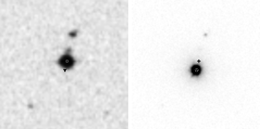
Figure 7.— Images of a $2\arcmin\times 2\arcmin$ field containing HAT-P-26 from the POSS-I Red survey (left), and from our FLWO 1.2 m $i$ band follow-up observations (right, see Section 2.4). North is up and east is to the left in both images. The dates of the exposures are 1950 April 21 and 2010 May 08, respectively. The cross marks the position of HAT-P-26 in 1950 and the triangle marks the position in 2010. Between these two dates HAT-P-26 has moved $\sim 8\farcs 9$ to the southeast. From the POSS-I image, we can rule out the presence of stars brighter than $R\sim 19$ at the current position of HAT-P-26.

3.2.3 Detailed blend modeling of a hierarchical triple

Figure 8.— Left: $\chi^{2}$ for the scenario of a binary star with a planet orbiting the fainter star (case 3 in Section 3.2.3) vs. the mass of the planet host. Points above the dotted horizontal line are rejected at the $3\sigma$ confidence level. The mass of the brightest star in the system is fixed to $0.788$ $M_{\sun}$ from the spectroscopically determined effective temperature, surface gravity and metallicity. Right: $\chi^{2}$ for the scenario of a binary star with a planet orbiting the brighter star (case 4 in Section 3.2.3) vs. the mass of the fainter star. We also show the radius of the planet (right axis). Points on the $\chi^{2}$ curve above the dotted horizontal line are rejected at the $3\sigma$ confidence level.

Following Bakos et al. (2010), Hartman et al. (2009), and Torres et al. (2005) we attempt to model the observations as a hierarchical triple system. We consider 4 possibilities:

1. One star orbited by a planet,

2. Three stars, 2 fainter stars are eclipsing,

3. Two stars, 1 planet, planet orbits the fainter star,

4. Two stars, 1 planet, planet orbits the brighter star.

Here case 1 is the fiducial model to which we compare the various blend models. We model the observed follow-up and HATNet light curves (including only points that are within one transit duration of the primary transit or secondary eclipse assuming zero eccentricity) together with the 2MASS and TASS photometry. In each case we fix the mass of the brightest star to $0.788$ $M_{\sun}$; this ensures that we reproduce the effective temperature, metallicity, and surface gravity determined from the SME analysis when using the Padova isochrones (see below). We have also attempted to perform the fits described below allowing the mass of the brightest star to vary. We find that in this case the mass of the brightest star is still constrained to be close to $0.788$ $M_{\sun}$ by the broad-band photometry, even if the spectroscopic parameters are not included. We therefore conclude that fixing the mass of the brightest star is justified. In all cases we vary the distance to the system and two parameters allowing for dilution in the two HATNet light curves, and we include simultaneous EPD and TFA in fitting the light curves (see Section 3.3). In each case we draw the stellar radii and magnitudes from the 13.0 Gyr Padova isochrone (Girardi et al., 2000), extended below 0.15 $M_{\sun}$ with the Baraffe et al. (1998) isochrones. We use these rather than the YY isochrones for this analysis because of the need to allow for stars with $M<0.4$ $M_{\sun}$, which is the lower limit available for the YY models. We use the JKTEBOP program (Southworth et al., 2004a, b) which is based on the Eclipsing Binary Orbit Program (EBOP; Popper & Etzel, 1981; Etzel, 1981; Nelson & Davis, 1972) to generate the model light curves. We optimize the free parameters using the Downhill Simplex Algorithm together with classical linear least squares for the EPD and TFA parameters. We rescale the errors for each light curve such that $\chi^{2}$ per degree of freedom is 1.0 for the out of transit portion of the light curve. Note that this is done prior to applying the EPD/TFA corrections, as a result $\chi^{2}$ per degree of freedom is less than 1.0 for each of the best-fit models discussed below. If the rescaling is not performed, the difference in $\chi^{2}$ between the best-fit models is even more significant than what is given below, and the blend-models may be rejected with higher confidence.

Case 1: 1 star, 1 planet: In addition to the parameters mentioned above, in this case we vary the radius of the planet and the impact parameter of the transit. The best-fit model has $\chi_{\rm Case1}^{2}=3140.1$ for 3567 degrees of freedom. The parameters that we obtain for the planet are comparable to those obtained from the global modelling described in Section 3.3.

Case 2: 3 stars: For case 2 we vary the masses of the eclipsing components, and the impact parameter of the eclipse. We find no model of three stars which reproduces the observations. The transit depth and duration cannot be fit when the three stars are constrained to fall on the same isochrone, and the brightest star has $M=0.788$ $M_{\sun}$. The best-fit case 2 model consists of equal masses for the brightest two stars, and $0.08$ $M_{\sun}$ (the lowest stellar mass in the Baraffe et al. 1998 isochrones) for the transiting star. Such a model is inconsistent with our spectroscopic observations (it would have been easily identified as a double-lined binary at one of the quadrature phases), and as we will show, can be rejected from the light curves alone. The best-fit case 2 model yields $\chi_{\rm Case2}^{2}=3310.2$ for 3566 degrees of freedom and produces model transits that are too deep compared to the observed transit. The case 1 model achieves a lower $\chi^{2}$ with fewer parameters than the case 2 model, so the case 1 model is preferred over the case 2 model. Assuming that the errors are uncorrelated and follow a Gaussian distribution, the case 2 model can be rejected in favor of the case 1 model at the $>116\sigma$ confidence level. Alternatively, one might suppose that any apparent correlations in the residuals of the best-fit case 2 model are not due to errors in the model but instead are due to uncorrected systematic errors in the measurements; large systematic errors in the measurements would increase the probability that case 1 might give a better fit to the data, by chance, than case 2. To establish the statistical signficance with which we may reject case 2 while allowing for possible systematic errors in the measurements, we conduct 1000 Monte Carlo simulations in which we assume the best-fit case 2 model scenario is correct, shuffle the residuals from this fit in a manner that preserves the correlations (this is done by taking the Fourier Transform of the residuals, randomly changing phases of the Transform while preserving the amplitudes, and transforming back to the time domain), and fit both the case 2 and case 1 models to the simulated data. The median value of $\chi^{2}_{\rm Case2}-\chi^{2}_{\rm Case1}$ is $-17.6$ with a standard deviation of $26.3$. None of the 1000 trials have $\chi^{2}_{\rm Case2}-\chi^{2}_{\rm Case1}>170.1$, the measured value. Based on this analysis we reject case 2, i.e. the hierarchical triple star system scenario, at the $7\sigma$ level.

Case 3: 2 stars, planet orbits the fainter star: In this scenario HAT-P-26b is a transiting planet, but it would have a radius that is larger than what we infer (it may be a Saturn- or Jupiter-size planet rather than a Neptune-size planet). For this case we vary the mass of the faint planet-hosting star, the radius of the planet, and the impact parameter of the transit. We assume the mass of the planet is negligible relative to the mass of its faint host star. Figure 8 shows $\chi^{2}$ as a function of the mass of the planet-hosting star for this scenario. The best-fit case 3 solution has $\chi^{2}=3147.6$ for 3566 degrees of freedom, and corresponds to a system where the two stars are of equal mass and the planet has a radius of $0.8$ $R_{\rm J}$. As the mass of the planet host is decreased the value of $\chi^{2}$ increases. Repeating the procedure outlined above to establish the statistical significance at which we may reject case 3 we find that the $3\sigma$ limit on $\chi^{2}_{\rm Case3}-\chi^{2}_{\rm Case1}$ is $9.0$, which results in a $3\sigma$ lower-limit of $0.77$ $M_{\sun}$ on the mass of the planet hosting star. We may thereby place a $3\sigma$ lower limit of $0.74$ on the $V$-band luminosity ratio of the two stars. A second set of lines with a luminosity ratio of $>0.74$ would have easily been detectable in both the Keck and TRES spectra unless the stars had very similar $\gamma$ velocities (the spectral lines are quite narrow with $v\sin{i}=1.8\pm 0.5\,\rm km\,s^{-1}$). The poor fit for this blend model relative to the fiducial model together with the tight constraints on the relative $\gamma$ velocities and luminosity ratios of the stars in the blend models that may yet fit the data leads us to reject this blend scenario in favor of the simpler model of a single star hosting a transiting planet.

Case 4: 2 stars, planet orbits the brighter star: As in the previous case, in this scenario HAT-P-26b is a transiting planet, but the dilution from the blending star means that the true radius is larger than what we infer in Case 1. In this case we vary the radius of the planet, the mass of the faint star, and the impact parameter of the transit. Again we assume the mass of the planet is negligible relative to the mass of its bright host star. Figure 8 shows $\chi^{2}$ as a function of the mass of the faint star. The smallest value of $\chi^{2}$ is achieved when the faint star contributes negligible light to the system, which is effectively equivalent to the fiducial scenario represented by Case 1. Two effects cause $\chi^{2}$ to increase with stellar mass. First, the shape of the transit is subtly changed in a manner that gives a poorer fit to the observations. Second, when the mass of the faint star is less than that of the transit host the model broad-band photometry for the blended system is redder than for the single star scenario, and is inconsistent with the observed photometry. This gives rise to the peak in $\chi^{2}$ at $M\sim 0.65$ $M_{\sun}$. The case 4 model where the faint star has $M\gtrsim 0.77$ $M_{\sun}$ can be rejected as in Case 3. For lower masses, we place a $3\sigma$ upper limit of 0.55 $M_{\sun}$ on the mass of the faint star, yielding a $3\sigma$ upper limit on the luminosity ratio of $0.1$. We conclude that at most the planet radius $R_{p}$ may be 8% larger than what we find in Section 3.3 if there is an undetected faint secondary star in the system.

3.3. Global modeling of the data

Here we summarize the procedure that we followed to model the HATNet photometry, the follow-up photometry, and the radial velocities simultaneously. This procedure is described in greater detail in Bakos et al. (2010). The follow-up light curves were modeled using analytic formulae based on Mandel & Agol (2002), with quadratic limb darkening coefficients for the Sloan $i$ band interpolated from the tables by Claret (2004) for the spectroscopic parameters of the star as determined from the SME analysis (Section 3.1). We modeled the HATNet data using an approximation to the Mandel & Agol (2002) formulae as described in Bakos et al. (2010). The RVs were fitted with an eccentric Keplerian model.

Our physical model consisted of 8 main parameters, including: the time of the first transit center observed with HATNet (taken to be event $-74$), $T_{c,-74}$, and that of the last transit center observed with the FLWO 1.2 m telescope, $T_{c,+40}$, the normalized planetary radius $p\equiv R_{p}/R_{\star}$, the square of the impact parameter $b^{2}$, the reciprocal of the half duration of the transit $\zeta/R_{\star}$ as given in Bakos et al. (2010), the RV semiamplitude $K$, and the Lagrangian elements $k\equiv e\cos\omega$ and $h\equiv e\sin\omega$, where $\omega$ is the longitude of periastron. Five additional parameters were included that have to do with the instrumental configuration. These are the HATNet blend factors $B_{\rm inst,376}$, and $B_{\rm inst,377}$, which account for possible dilution of the transit in the HATNet light curves from background stars due to the broad PSF ($\sim 24\arcsec$ FWHM), the out-of-transit magnitudes for each HATNet field, $M_{\rm 0,HATNet,376}$ and $M_{\rm 0,HATNet,377}$, and the relative zero-point $\gamma_{\rm rel}$ of the Keck RVs. The physical model was extended with an instrumental model for the follow-up light curves that describes brightness variations caused by systematic errors in the measurements. We adopted a “local” EPD- and “global” TFA-model (Bakos et al., 2010), using 20 template stars for the TFA procedure and six EPD parameters for each follow-up light curve. In summary, the total number of fitted parameters was 13 (physical model with 5 configuration-related parameters) + 30 (local EPD) + 20 (global TFA) = 63, i.e., much smaller than the number of data points (1450, counting only RV measurements and follow-up photometry measurements).

As described in Bakos et al. (2010), we use a combination of the downhill simplex method (AMOEBA; see Press et al., 1992), the classical linear least squares algorithm, and the Markov Chain Monte-Carlo method (MCMC, see Ford, 2006) to obtain a best-fit model together with a posteriori distributions for the fitted parameters. These distributions were then used to obtain a posteriori distributions for other quantities of interest, such as $\rho_{\star}$. As described in Section 3.1, $\rho_{\star}$ was used together with stellar evolution models to obtain a posteriori distributions for stellar parameters, such as $M_{\star}$ and $R_{\star}$, which are needed to determine $M_{p}$ and $R_{p}$.

The resulting parameters pertaining to the light curves and velocity curves, together with derived physical parameters of the planet, are listed under the “Adopted Value” column heading of Table 5. Included in this table is the RV “jitter”. This is a component of assumed astrophysical noise intrinsic to the star, possibly with a contribution from instrumental errors as well, that we added in quadrature to the internal errors for the RVs in order to achieve $\chi^{2}/{\rm dof}=1$ from the RV data for the global fit. Auxiliary parameters not listed in the table are: $T_{\mathrm{c},-74}=2454860.02709\pm 0.00147$ (BJD), $T_{\mathrm{c},+40}=2455342.76185\pm 0.00041$ (BJD), the blending factors $B_{\rm instr,376}=0.92\pm 0.05$, and $B_{\rm instr,377}=0.84\pm 0.10$ for the HATNet field 376 and 377 light curves, respectively, and $\gamma_{\rm rel}=-2.8\pm 0.8$ $\rm m\,s^{-1}$. The latter quantity represents an arbitrary offset for the Keck RVs, but does not correspond to the true center-of-mass velocity of the system, which was listed earlier as $\gamma_{\rm RV}$ in Table 4.

We find a mass for the planet of $M_{p}=0.059\pm 0.007\,M_{\rm J}$ and a radius of $R_{p}=0.565_{-0.032}^{+0.072}\,R_{\rm J}$, leading to a mean density $\rho_{p}=0.40\pm 0.10$ $\rm g\,cm^{-3}$. We also find that the eccentricity of the orbit may be different from zero: $e=0.124\pm 0.060$, $\omega=54\pm 165\arcdeg$. However, as we show in Section 4.3, this is at best significant at only the 88% confidence level.

We also carried out the analysis described above with the eccentricity fixed to zero. The resulting parameters are given in Table 5 under the column heading “$\{\zeta/R_{\star},b^{2},p\},e\equiv 0$”. The results are discussed further in Section 4.3.

Finally, we conducted an independent model of the system based on Kipping & Bakos (2010b). The primary differences between this model and the adopted model are differences in the choice of parameters to vary in the fit: we use $\Upsilon/R_{\star}$ as defined in Kipping & Bakos (2010b) rather than $\zeta/R_{\star}$, $b$ rather than $b^{2}$, and $p^{2}$ rather than $p$. We also allowed for a linear drift in the radial velocities $\dot{\gamma}$, and a time shift $t_{\rm troj}$ in the radial velocities due to possible additional bodies in the system on Trojan orbits with HAT-P-26b. We chose to include both $t_{\rm troj}$ and $\dot{\gamma}$ rather than fixing them to zero as the value of the Bayseian Information Criterion (BIC; e.g. Kipping et al., 2010) was lower for the best-fit model including these parameters, than for models where one or both of these parameters were fixed to zero. The resulting parameters are given in Table 5 under the column heading “$\{\Upsilon/R_{\star},b,p^{2}\}$.” The parameter values from this model are consistent with those from the adopted model, which gives confidence that our results are robust to changes in the choice of fitting parameters.

Table 5Orbital and planetary parameters

Parameter	Adopted Value	Value	Value
	$\{\zeta/R_{\star},b^{2},p\}$	$\{\zeta/R_{\star},b^{2},p\},e\equiv 0$	$\{\Upsilon/R_{\star},b,p^{2}\}$
Light curve parameters
$P$ (days)	$4.234516\pm 0.000015$	$4.234515\pm 0.000015$	$4.234508_{-0.000022}^{+0.000021}$
$T_{c}$ (${\rm BJD}$)	$2455304.65122\pm 0.00035$	$2455304.65118\pm 0.00036$	$2455304.65120_{-0.00049}^{+0.00048}$
$T_{14}$ (days)	$0.1023\pm 0.0010$	$0.1025\pm 0.0010$	$0.1023_{-0.0011}^{+0.0012}$
$T_{12}=T_{34}$ (days)	$0.0077\pm 0.0007$	$0.0078\pm 0.0007$	$0.00724_{-0.00027}^{+0.00081}$
$a/R_{\star}$	$13.06\pm 0.83$	$13.44_{-0.59}^{+0.44}$	$13.28_{-0.76}^{+0.70}$
$\zeta/R_{\star}$	$21.15\pm 0.16$	$21.14\pm 0.16$	$21.10_{-0.21}^{+0.20}$
$R_{p}/R_{\star}$	$0.0737\pm 0.0012$	$0.0738\pm 0.0012$	$0.07341_{-0.00093}^{+0.00104}$
$b^{2}$	$0.092_{-0.053}^{+0.087}$	$0.110_{-0.059}^{+0.076}$	$0.035_{-0.032}^{-0.089}$
$b\equiv a\cos i/R_{\star}$	$0.303_{-0.122}^{+0.112}$	$0.332_{-0.123}^{+0.095}$	$0.00_{-0.00}^{+0.26}$
$i$ (deg)	$88.6_{-0.9}^{+0.5}$	$88.6\pm 0.5$	$89.14_{-0.72}^{+0.59}$
Limb-darkening coefficients
$a_{i}$ (linear term)	$0.3862$	$0.3862$	$0.3862$
$b_{i}$ (quadratic term)	$0.2576$	$0.2576$	$0.2576$
RV parameters
$K$ ($\rm m\,s^{-1}$)	$8.5\pm 1.0$	$8.3\pm 1.0$	$7.6_{-1.2}^{+1.2}$
$k_{\rm RV}$	$0.099\pm 0.060$	$0.000\pm 0.000$	$0.09_{-0.11}^{+0.12}$
$h_{\rm RV}$	$0.027\pm 0.076$	$0.000\pm 0.000$	$0.028_{-0.060}^{+0.063}$
$e$	$0.124\pm 0.060$	$0.000\pm 0.000$	$0.127_{-0.068}^{+0.094}$
$\omega$ (deg)	$54\pm 165$	$0\pm 0$	$74_{-59}^{+266}$
$\dot{\gamma}$ (m s-1 d-1)	$0$	$0$	$-0.028_{-0.013}^{+0.014}$
$t_{\rm troj}$ (d)	$0$	$0$	$0.01_{-0.23}^{+0.24}$
RV jitter ($\rm m\,s^{-1}$)	$1.6$	$2.4$	$\ldots$
RV fit RMS ($\rm m\,s^{-1}$)	$2.4$	$3.0$	$\ldots$
Secondary eclipse parameters
$T_{s}$ (BJD)	$2455307.037\pm 0.162$	$2455306.768\pm 0.000$	$2455307.01_{-0.29}^{+0.31}$
$T_{s,14}$	$0.1074\pm 0.0162$	$0.1025\pm 0.0010$	$0.108_{-0.011}^{+0.014}$
$T_{s,12}$	$0.0082\pm 0.0067$	$0.0078\pm 0.0007$	$0.00782_{-0.00083}^{+0.00104}$
Planetary parameters
$M_{p}$ ($M_{\rm J}$)	$0.059\pm 0.007$	$0.057\pm 0.007$	$0.0522_{-0.0083}^{+0.0084}$
$R_{p}$ ($R_{\rm J}$)	$0.565_{-0.032}^{+0.072}$	$0.549_{-0.023}^{+0.034}$	$0.553_{-0.031}^{+0.037}$
$C(M_{p},R_{p})$	$0.07$	$0.08$	$0.059$
$\rho_{p}$ ($\rm g\,cm^{-3}$)	$0.40\pm 0.10$	$0.42\pm 0.08$	$0.378_{-0.084}^{+0.099}$
$\log g_{p}$ (cgs)	$2.65_{-0.10}^{+0.08}$	$2.67\pm 0.07$	$2.621_{-0.092}^{+0.084}$
$a$ (AU)	$0.0479\pm 0.0006$	$0.0478\pm 0.0006$	$0.04780_{-0.00061}^{+0.00064}$
$T_{\rm eq}$ (K)	$1001_{-37}^{+66}$	$981\pm 29$	$991_{-36}^{+42}$
$\Theta$	$0.012\pm 0.002$	$0.012\pm 0.002$	$0.0110_{-0.0019}^{+0.0020}$
$F_{peri}$ ($10^{8}$$\rm erg\,s^{-1}\,cm^{-2}$)	$2.91_{-0.48}^{+7.54}$	$2.10_{-0.20}^{+0.30}$	$2.87_{-0.63}^{+1.03}$
$F_{ap}$ ($10^{8}$$\rm erg\,s^{-1}\,cm^{-2}$)	$1.81\pm 0.32$	$2.10_{-0.20}^{+0.30}$	$1.72_{-0.31}^{+0.28}$
$\langle F\rangle$ ($10^{8}$$\rm erg\,s^{-1}\,cm^{-2}$)	$2.27_{-0.31}^{+1.08}$	$2.10_{-0.20}^{+0.30}$	$2.18_{-0.30}^{+0.40}$

4. Discussion

We have presented the discovery of HAT-P-26b, a transiting Neptune-mass planet. Below we discuss the physical properties of this planet, and compare them to the properties of similar planets; we comment on the possibility that the planet has undergone significant evaporation, on the significance of its orbital eccentricity, and on the possible presence of additional bodies in the system; and we discuss the prospects for detailed follow-up studies.

4.1. Physical Properties of HAT-P-26b

Figure 9 compares HAT-P-26b to the other known TEPs on a mass-radius diagram. With a density of $0.40\pm 0.10$ $\rm g\,cm^{-3}$, HAT-P-26b is significantly less dense than the four other Neptune-size planets with well measured masses and radii (Uranus, Neptune, GJ 436b, HAT-P-11b). For Kepler-4b, Kipping & Bakos (2010a) find a large uncertainty on the radius which results from significant uncertainties on the eccentricity and the transit impact parameter. Kepler-4b may be comparable in size to GJ 436b and HAT-P-11b, or it could be even less dense than HAT-P-26b.

From the theoretical models of Fortney et al. (2007), HAT-P-26b has a radius that is well above the maximum radius of $0.3$ $R_{\rm J}$ for a $0.06$ $M_{\rm J}$ planet lacking a hydrogen-helium envelope (i.e. a planet with a 100% water-ice composition). The best-fit mass and radius for HAT-P-26b falls just below the 4 Gyr model with a 10 $M_{\earth}$ rocky core and 8 $M_{\earth}$ gas envelope, implying that a 4 Gyr model with a slightly higher core mass would provide a better match to the mass and radius. We note that the isochrone-based age ($9.0_{-4.9}^{+3.0}$ Gyr) and the activity-based age ($7.8^{+1.4}_{-1.2}$ Gyr) for the HAT-P-26 system are somewhat older than 4 Gyr, so the inferred core-mass would therefore be somewhat smaller.

We also compare HAT-P-26b to the theoretical models of Baraffe et al. (2008) which predict more significant inflation due to irradiation for low mass planets than do the Fortney et al. (2007) models. In this case the radius of HAT-P-26b is intermediate between the $Z=0.5$ and $Z=0.9$ heavy-element enrichment models.

4.2. Evaporation

Observations of the transiting hot Jupiters HD 209458b and HD 189733b in the H I Lyman-$\alpha$ line have indicated that both planets are evaporating at a rate of up to $\sim 10^{10}$ g s^-1 (e.g, Vidal-Madjar et al., 2003; Lecavelier des Etangs et al., 2010). Prompted by the observations for HD 209458b, several theoretical studies have indicated that atmospheric evaporation is likely to be important for close-in planets, particularly those with low surface gravities, such as hot Neptunes (see for example Lammer et al., 2003 and the review by Yelle et al., 2008). It has even been suggested that some close-in Neptune-mass and smaller planets may be the evaporated cores of planets which initially had masses comparable to Saturn or Jupiter (e.g. Baraffe, 2005). In the case of energy-limited escape, the evaporative mass-loss is given by (see Erkaev et al., 2007, and Yelle et al., 2008; see also Valencia et al., 2010 and Jackson et al., 2010 for applications to CoRoT-7b):

$$\dot{M_{p}}=-\frac{\pi R_{p}^{3}\epsilon F_{\rm XUV}}{GM_{p}K_{\rm tide}}$$ (1)

where $F_{\rm XUV}$ is the incident flux of extreme ultraviolet (XUV) stellar radiation, $\epsilon$ is the heating efficiency and is estimated to be $\sim 0.4$ for the case of HD 209458b (Yelle et al., 2008), and $K_{\rm tide}$ is a factor that accounts for an enhancement of the evaporation rate in the presence of tides, and is given by:

$$K_{\rm tide}=1-\frac{3}{2\xi}+\frac{1}{2\xi^{3}}$$ (2)

where $\xi=(M_{p}/(3M_{\star}))^{1/3}a/R_{p}$ is the ratio of the Roche radius to the planet radius. Ribas et al. (2005) find that for solar type stars the XUV flux at 1 AU integrated over the wavelength range $1$ Å to $1200$ Å is given by:

$$F_{\rm XUV,1AU}=29.7\tau^{-1.23}\,{\rm ergs}\,{\rm s}^{-1}\,{\rm cm}^{-2}$$ (3)

where $\tau$ is the age in Gyr. To our knowledge, a similar study has not been completed for K dwarfs, however long term X-ray observations of the 5-6 Gyr $\alpha$ Cen AB system reveal that on average the K1 dwarf star $\alpha$ Cen B has an X-ray luminosity in the 6-60 Å band that is approximately twice that of the Sun, while the G2 dwarf $\alpha$ Cen A has a luminosity that is approximately half that of the Sun (Ayers, 2009). For simplicity we therefore assume that the total XUV luminosity of HAT-P-26 is comparable to that of the Sun (4.64 ergs s^-1 cm^-2 at 1 AU; Ribas et al., 2005), which is likely correct to within an order of magnitude. Assuming $\epsilon=0.4$, we estimate that the expected present-day mass-loss rate for HAT-P-26b is $\sim 3\times 10^{10}\,{\rm g}\,{\rm s}^{-1}=0.17\,M_{\earth}\,{\rm Gyr}^{-1}$. To determine the total mass lost by HAT-P-26b over its lifetime, we integrate equation 1 assuming an age of $4.5$ Gyr, $F\propto\tau^{-1.23}$ for $\tau>0.1$ Gyr and $F\equiv{\rm constant}$ for $\tau<0.1$ Gyr, neglecting tidal evolution of the orbit, and assuming that the radius is constant. We find that HAT-P-26b may have lost a significant fraction its mass ($\sim$ 30%); the exact value depends strongly on several poorly constrained parameters including $F_{\rm XUV}$ and its dependence on age for a K1 dwarf, $\epsilon$, and the age of the system.

4.3. Eccentricity

Using the relation given by Adams & Laughlin (2006), the expected tidal circularization time-scale for HAT-P-26b is $\sim 1$ Gyr which is much less than the age of the system. This time-scale is estimated assuming a large tidal quality factor of $Q_{P}=10^{6}$, and that there are no additional bodies in the system exciting the eccentricity. However, because at least two of the three hot Neptunes have significant eccentricities (GJ 436b has $e=0.14\pm 0.01$, Demory et al., 2007; and HAT-P-11b has $e=0.198\pm 0.046$, Bakos et al., 2010; the eccentricity for Kepler-4b is poorly constrained, Kipping & Bakos, 2010a), we cannot conclude that the eccentricity must be zero on physical grounds, and therefore do not adopt a zero-eccentricity model for the parameter determination.

As discussed in Section 3.1 the eccentricity of HAT-P-26b is poorly constrained by the RV observations, and is instead constrained by requiring that the star be younger than the age of the universe (without the age constraint we get $e=0.24\pm 0.12$, whereas including the age constraint gives $e=0.124\pm 0.060$). To establish the significance of the eccentricity measurement, we also fit a model with the eccentricity fixed to zero. An F-test (e.g. Lupton, 1993) allows us to reject the null hypothesis of zero eccentricity with only 79% confidence. Alternatively, the Lucy & Sweeney (1971) test for the significance of an eccentricity measurement gives a false alarm probability of $\sim 12$% for detecting $e>0.124$ with an error of $0.060$, or 88% confidence that the orbit is eccentric. If the eccentricity is fixed to zero, the required jitter to achieve $\chi^{2}/N_{\rm dof}=1$ is 2.4 $\rm m\,s^{-1}$, which is closer to the typical Keck/HIRES jitter of other chromospherically quiet early K dwarfs than the jitter of $1.6$ $\rm m\,s^{-1}$ that is obtained with an eccentric orbit fit. We therefore are not able to claim a significant eccentricity for HAT-P-26b, and instead may only place a $95\%$ confidence upper limit of $e<0.22$. For the $\{\Upsilon/R_{\star},b,p^{2}\}$ model discussed at the end of Section 3.3, the $95\%$ confidence upper limit is $e<0.32$. Further RV observations, or a photometric detection of the occultation of the planet by its host star, are needed to determine if the eccentricity is nonzero.

4.4. Additional Bodies in the System

The $\{\Upsilon/R_{\star},b,p^{2}\}$ model discussed in Section 3.3 with parameters given in Table 5 includes a linear drift in the radial velocities, $\dot{\gamma}$, as a free parameter. We find $\dot{\gamma}=-0.028_{-0.013}^{+0.014}$ m s^-1 d^-1. Conducting an odds ratio test (see Kipping et al., 2010), we conclude that the drift is real with 96.6% confidence, making this a $2.1\sigma$ detection. While the detection is not significant enough for us to be highly confident that there is at least one additional body in the system, this suggestive result implies that HAT-P-26 warrants long-term RV monitoring. We also searched for a linear time-shift in the RVs due to potential Trojans. We do not detect a significant shift, and may exclude $|t_{\rm troj}|<0.50$ d with 95% confidence. This translates to an upper limit of $84$ $M_{\earth}$ on the mass of a Trojan companion, which is greater than the mass of the planet. With the present data we are thus not able to place a meaningful limit on the presence of Trojan companions.

4.5. Suitability for Follow-up

HAT-P-26 has a number of features that make it an attractive target for potential follow-up studies. At $V=11.744$, it is bright enough that precision spectroscopic and photometric observations are feasible with moderate integration times. The equatorial declination of $\delta=+04{\arcdeg}03{\arcmin}36.0{\arcsec}$ also means that HAT-P-26 is accessible to both Northern and Southern ground-based facilities. The exceptionally low jitter will facilitate further RV observations, which might be used to confirm and refine the eccentricity determination, to measure the Rossiter-McLaughlin effect (R-M; discussed in more detail below) and to search for additional planets in the system.

A detection of the occultation of HAT-P-26b by HAT-P-26 with IRAC/Spitzer would provide a strong constraint on $k\equiv e\cos\omega$, while the duration of the occultation would provide a constraint on $h\equiv e\sin\omega$. We note that the median value of the a posteriori distribution for the time of occultation that results from our global fit when the eccentricity is allowed to vary (Section 3.3) is $6.5$ h after the expected time of occultation assuming a circular orbit. The expected depth of the occultation event is a challenging $0.012\%$ and $0.020\%$ at 3.6 µm and 4.5 µm respectively. Scaling from TrES-4, a somewhat fainter star at these wavelengths, for which Knutson et al. (2009) measured occultations at 3.6 µm and 4.5 µm using IRAC/Spitzer with precisions of $0.011\%$ and $0.016\%$ respectively, one may hope to achieve a $\sim 1.4\sigma$ and $1.6\sigma$ detection for HAT-P-26b for one event at each bandpass. One would need to observe 5 and 4 occultations respectively to achieve a $3\sigma$ detection.

Recent measurements of the R-M effect for TEPs have revealed a substantial population of planets on orbits that are significantly misaligned with the spin axes of their host stars (e.g. Triaud et al., 2010). Winn et al. (2010a) note that misalignment appears to be more prevalent for planets orbiting stars with $T_{\rm eff}>6250$ K, and suggest that most close-in planets migrate by planet-planet or planet-star scattering mechanisms, or by the Kozai effect, rather than disk migration, and that tidal dissipation in the convective surfaces of cooler stars realigns the stellar spin axis to the orbital axis of the close-in massive planet. Schlaufman (2010) also finds evidence that planets orbiting stars with $M_{\star}>1.2$ $M_{\sun}$ are more likely to be misaligned than planets orbiting cooler stars using a method that is independent of the R-M measurements. One prediction of the Winn et al. (2010a) hypothesis is that lower mass planets orbiting cool stars should show a greater degree of misalignment than higher mass planets due to their reduced tidal influence. The detection of misalignment for HAT-P-11b (Winn et al., 2010b; Hirano et al., 2010) is consistent with this hypothesis. Measuring the R-M effect for HAT-P-26b would provide an additional test. Using equation (40) from Winn (2010), the expected maximum amplitude of the R-M effect for HAT-P-26b is $\sim 9$ $\rm m\,s^{-1}$, which given the low jitter of HAT-P-26, should be detectable at $\gtrsim 10\sigma$.

By measuring the primary transit depth as a function of wavelength it is possible to obtain a transmission spectrum of an exoplanet’s atmosphere. Such observations have been made for a handful of planets (e.g. Charbonneau et al., 2002; see also the review by Seager & Deming, 2010). Following Brown (2001), the expected difference in transit depth between two wavelengths is given approximately by:

$$\Delta\delta=\frac{2R_{p}H}{R_{\star}^{2}}N_{H}$$ (4)

where $H=k_{\rm B}T_{\rm eq}/g_{p}\mu$ is the scale height of the atmosphere, $g_{p}$ is the planet surface gravity, $\mu$ is the mean molecular weight of the atmosphere, and $N_{H}=\ln(\sigma_{1}/\sigma_{2})$ where $\sigma_{1}$ and $\sigma_{2}$ are the opacities per gram of material at wavelengths in a strong atomic or molecular line and in the nearby continuum respectively. Assuming a pure H₂ atmosphere, $\mu=3.347\times 10^{-27}$ kg, we find for HAT-P-26b $H=920$ km, and $\Delta\delta=0.0246N_{H}\%$. If instead we assume that the atmosphere has the same composition as Neptune (e.g. de Pater & Lissauer, 2001), we have $\mu=4.655\times 10^{-27}$ kg, $H=660$ km, and $\Delta\delta=0.0177N_{H}\%$. For comparison, assuming a pure H₂ atmosphere, the planet HD 209458b has $\Delta\delta=0.0198N_{H}\%$, while GJ 436b has $\Delta\delta=0.0107N_{H}\%$, HAT-P-11b has $\Delta\delta=0.0072N_{H}\%$ and Kepler-4b has $\Delta\delta=0.0038N_{H}\%$. Due to its low surface gravity, HAT-P-26b easily has the highest expected transmission spectrum signal among the known transiting Neptune-mass planets. While it is relatively faint compared to the well studied planets HD 209458b and HD 189733b, we note that Sing et al. (2010) used the Gran Telescopio Canarias (GTC) to detect a $0.058\pm 0.016\%$ absorption level at 7582 Å due to Potassium in the atmosphere of XO-2b, which orbits a $V=11.2$ early K star. Scaling from this observation, it should be possible to detect components in the atmosphere of HAT-P-26b with $N_{H}\gtrsim 3$ at the $\sim 3\sigma$ level using the GTC.

4.6. Summary

In summary, HAT-P-26b is a low-density Neptune-mass planet. Its low-density relative to the other known Neptune-mass planets means that HAT-P-26b likely has a more significant hydrogen-helium gas envelope than its counterparts. The existence of HAT-P-26b provides empirical evidence that, like hot Jupiters, hot Neptunes also exhibit a wide range of densities. Comparing to the Fortney et al. (2007) models, we find that HAT-P-26b is likely composed of a gas envelope and a heavy-element core that are approximately equal in mass, while the Baraffe et al. (2008) models prefer a higher heavy-element fraction. It is also likely that irradiation-driven mass-loss has played a significant role in the evolution of HAT-P-26b –we find that the planet may have lost $\sim 30\%$ of its present-day mass over the course of its history, though this conclusion depends strongly on a number of very poorly constrained parameters, particularly the XUV flux of HAT-P-26 and its evolution in time. We place a 95% confidence upper limit on the eccentricity of $e<0.22$. If further observations detect a nonzero eccentricity, it would mean that at least three of the four known Neptune-mass TEPs have nonzero eccentricities, which may imply that the tidal quality factor is higher than expected for these planets. Observations of the planetary occultation event for HAT-P-26b with IRAC/Spitzer would greatly constrain the eccentricity, however the low expected depth is likely to make this a challenging observation. We find suggestive evidence for a linear drift in the RVs which is significant at the $2.1\sigma$ level. If confirmed, this would imply the existence of at least one additional body in the HAT-P-26 system. With an expected R-M amplitude of $\sim 9$ $\rm m\,s^{-1}$ and a low stellar RV jitter, HAT-P-26b is a good target to measure the R-M effect and thereby test the hypothesis that low-mass planets are more likely to be misaligned than high-mass planets. The low surface gravity also makes HAT-P-26b a good target for transmission spectroscopy.

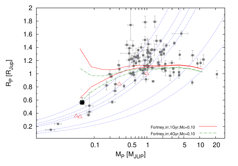
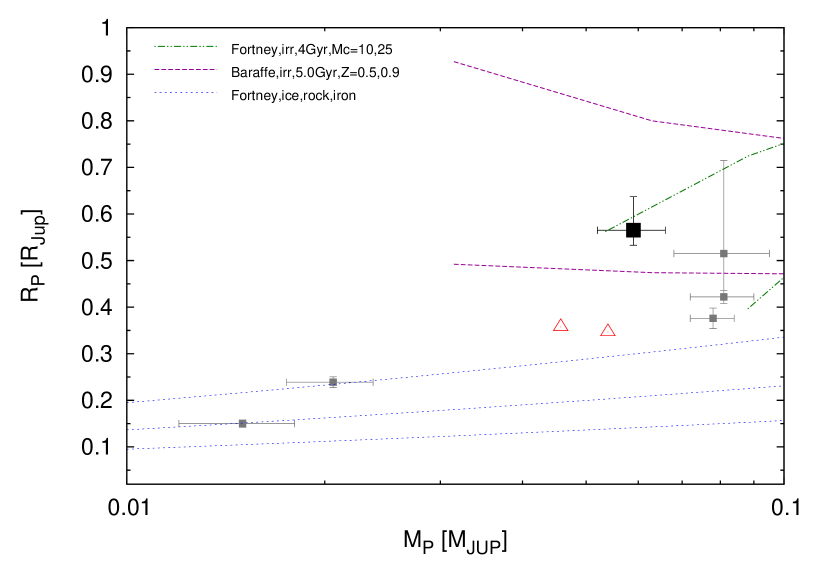
Figure 9.— Top: Mass–radius diagram of known TEPs (small filled squares). HAT-P-26b is shown as a large filled square. Overlaid are Fortney et al. (2007) theoretical planetary mass–radius curves interpolated to the solar equivalent semi-major axis of HAT-P-26b for ages of 1.0 Gyr (upper, solid lines) and 4 Gyr (lower dashed-dotted lines) and core masses of 0 and 10 $M_{\earth}$(upper and lower lines respectively), as well as isodensity lines for 0.4, 0.7, 1.0, 1.33, 5.5 and 11.9 $\rm g\,cm^{-3}$(dashed lines). Solar system planets are shown with open triangles. Bottom: Mass–radius diagram for planets with $0.01\,M_{\rm J}<M_{p}<0.1\,M_{\rm J}$. References for the low-mass planet parameters are given in Section 1 of the text. We adopt the “a.e” model from Kipping & Bakos (2010a) for Kepler-4b. Overlaid are the interpolated Fortney et al. (2007) theoretical relations for 4 Gyr and core masses of 10 and 25 $M_{\earth}$, Fortney et al. (2007) theoretical curves for pure ice, rock and iron composition planets (upper, middle, and lower dotted lines), and the Baraffe et al. (2008) theoretical irradiated curves for heavy element mass fractions of $Z=0.5$ and $0.9$ (upper and lower dashed lines respectively).

References

- Adams & Laughlin (2006) Adams, F. C., & Laughlin, G. 2006, ApJ, 649, 1004
- Ayers (2009) Ayers, T. R. 2009, ApJ, 696, 1931
- Bakos et al. (2004) Bakos, G. Á., Noyes, R. W., Kovács, G., Stanek, K. Z., Sasselov, D. D., & Domsa, I. 2004, PASP, 116, 266
- Bakos et al. (2007) Bakos, G. Á., et al. 2007, ApJ, 670, 826
- Bakos et al. (2010) Bakos, G. Á., et al. 2010, ApJ, 710, 1724
- Baraffe et al. (1998) Baraffe, I., Chabrier, G., Allard, F., & Hauschildt, P. H. 1998, A&A, 337, 403
- Baraffe (2005) Baraffe, I., Chabrier, G., Barman, T. S., Selsis, F., Allard, F., & Hauschildt, P. H. 2005, A&A, 436, L47
- Baraffe et al. (2008) Baraffe, I., Chabrier, G., & Barman, T. 2008, A&A, 482, 315
- Borucki et al. (2010) Borucki, W. J., et al. 2010, ApJ, 713, L126
- Brown (2001) Brown, T. M. 2001, ApJ, 553, 1006
- Buchhave et al. (2010) Buchhave, L. A., et al. 2010, ApJ, 720, 1118
- Butler et al. (1996) Butler, R. P. et al. 1996, PASP, 108, 500
- Butler et al. (2004) Butler, R. P., Vogt, S. S., Marcy, G. W., Fischer, D. A., Wright, J. T., Henry, G. W., Laughlin, G., & Lissauer, J. J. 2004, ApJ, 617, 580
- Carpenter (2001) Carpenter, J. M. 2001, AJ, 121, 2851
- Charbonneau et al. (2002) Charbonneau, D., Brown, T. M., Noyes, R. W., & Gilliland, R. L. 2002, ApJ, 568, 377
- Charbonneau et al. (2009) Charbonneau, D., et al. 2009, Nature, 462, 891
- Claret (2004) Claret, A. 2004, A&A, 428, 1001
- Demory et al. (2007) Demory, B.-O., et al. 2007, A&A, 475, 1125
- de Pater & Lissauer (2001) de Pater, I., & Lissauer, J. J. 2001, Planetary Sciences, p. 80. ISBN 0521482194. Cambridge, UK: Cambridge University Press, December 2001.
- Droege et al. (2006) Droege, T. F., Richmond, M. W., & Sallman, M. 2006, PASP, 118, 1666
- Erkaev et al. (2007) Erkaev, N. V., Kulikov, Y. N., Lammer, H., Selsis, F., Langmayr, D., Jaritz, G. F., & Biernat, H. K. 2007, A&A, 472, 329
- Etzel (1981) Etzel, P. B. 1981, NATO ASI, p. 111
- Ford (2006) Ford, E. 2006, ApJ, 642, 505
- Fortney et al. (2007) Fortney, J. J., Marley, M. S., & Barnes, J. W. 2007, ApJ, 659, 1661
- Fűrész (2008) Fűrész, G. 2008, Ph.D. thesis, University of Szeged, Hungary
- Gillon et al. (2007) Gillon, M., et al. 2007, A&A, 472, L13
- Girardi et al. (2000) Girardi, L., Bressan, A., Bertelli, G., & Chiosi, C. 2000, A&AS, 141, 371
- Hansen & Barman (2007) Hansen, B. M. S., & Barman, T. 2007, ApJ, 671, 861
- Hartman et al. (2009) Hartman, J. D., et al. 2009, ApJ, 706, 785
- Hartman et al. (2010) Hartman, J. D., et al. 2010, ApJ, submitted, arXiv:1007.4850
- Hirano et al. (2010) Hirano, T., Narita, N., Shporer, A., Sato, B., Aoki, W., & Tamura, M. 2010, PASJ, submitted, arXiv:1009.5677
- Holman et al. (2010) Holman, M. J., et al. 2010, Science, in press
- Isaacson & Fischer (2010) Isaacson, H., & Fischer, D. A. 2010, ApJ, in press, arXiv:1009.2301
- Jackson et al. (2010) Jackson, B., Miller, N., Barnes, R., Raymond, S. N., Fortney, J. J., & Greenberg, R. 2010, MNRAS, 407, 910
- Kipping & Bakos (2010a) Kipping, D. M., & Bakos, G. Á. 2010a, arXiv:1004.3538
- Kipping & Bakos (2010b) Kipping, D. M., & Bakos, G. Á. 2010b, arXiv:1006.5680
- Kipping et al. (2010) Kipping, D. M., et al. 2010, ApJ, submitted, arXiv:1008.3389
- Knutson et al. (2009) Knutson, H. A., Charbonneau, D., Burrows, A., O’Donovan, F. T., & Mandushev, G. 2009, ApJ, 691, 866
- Komatsu et al. (2010) Komatsu, E., et al. 2010, ApJS submitted, arXiv:1001.4538
- Kovács et al. (2002) Kovács, G., Zucker, S., & Mazeh, T. 2002, A&A, 391, 369
- Kovács et al. (2005) Kovács, G., Bakos, G. Á., & Noyes, R. W. 2005, MNRAS, 356, 557
- Kurtz (1985) Kurtz, D. W. 1985, MNRAS, 213, 773
- Lammer et al. (2003) Lammer, H., Selsis, F., Ribas, I., Guinan, E. F., Bauer, S. J., & Weiss, W. W. 2003, ApJ, 598, L121
- Lecavelier des Etangs et al. (2010) Lecavelier des Etangs, A., et al. 2010, A&A, in press, arXiv:1003.2206
- Léger et al. (2009) Léger, A., et al. 2009, A&A, 506, 287
- Lucy & Sweeney (1971) Lucy, L. B., & Sweeney, M. A. 1971, AJ, 76, 544
- Lupton (1993) Lupton, R. 1993, “Statistics in Theory and Practice”, Princeton N.J.: Princeton University Press, p. 100
- Mamajek & Hillenbrand (2008) Mamajek, E. E., & Hillenbrand, L. A. 2008, ApJ, 687, 1264
- Mandel & Agol (2002) Mandel, K., & Agol, E. 2002, ApJ, 580, L171
- Marcy & Butler (1992) Marcy, G. W., & Butler, R. P. 1992, PASP, 104, 270
- Nelson & Davis (1972) Nelson, B., & Davis, W. D. 1972, ApJ, 174, 617
- Noyes et al. (1984) Noyes, R. W., Hartmann, L. W., Baliunas, S. L., Duncan, D. K., & Vaughan, A. H. 1984, ApJ, 279, 763
- Pál & Bakos (2006) Pál, A., & Bakos, G. Á. 2006, PASP, 118, 1474
- Pál et al. (2008) Pál, A., et al. 2008, ApJ, 680, 1450
- Pál (2009b) Pál, A. 2009b, arXiv:0906.3486, PhD thesis
- Popper & Etzel (1981) Popper, D. M., & Etzel, P. B. 1981, AJ, 86, 102
- Press et al. (1992) Press, W. H., Teukolsky, S. A., Vetterling, W. T. & Flannery, B. P., 1992, Numerical Recipes in C: the art of scientific computing, Second Edition, Cambridge University Press
- Queloz et al. (2001) Queloz, D. et al. 2001, A&A, 379, 279
- Queloz et al. (2009) Queloz, D., et al. 2009, A&A, 506, 303
- Quinn et al. (2010) Quinn, S. N., et al. 2010, ApJsubmitted, arXiv:1008.3565
- Ramírez & Meléndez (2005) Ramírez, I., & Meléndez, J. 2005, ApJ, 626, 465
- Ribas et al. (2005) Ribas, I., Guinan, E. F., Güdel, M., & Audard, M. 2005, ApJ, 622, 680
- Roeser et al. (2010) Roeser, S., Demleitner, M., & Schilbach, E. 2010, AJ, 139, 2440
- Schlaufman (2010) Schlaufman, K. C. 2010, ApJ, 719, 602
- Seager & Mallén-Ornelas (2003) Seager, S., & Mallén-Ornelas, G. 2003, ApJ, 585, 1038
- Seager & Deming (2010) Seager, S., & Deming, D. 2010, ARA&A, 48, 631
- Seidelmann et al. (2007) Seidelmann, P. K., et al. 2007, Celest. Mech. Dyn. Astron., 98, 155
- Sing et al. (2010) Sing, D. K. 2010, A&A submitted, arXiv:1008.4795
- Skrutskie et al. (2006) Skrutskie, M. F., et al. 2006, AJ, 131, 1163
- Southworth et al. (2004a) Southworth, J., Maxted, P. F. L., & Smalley, B. 2004a, MNRAS, 351, 1277
- Southworth et al. (2004b) Southworth, J., Zucker, S., Maxted, P. F. L., & Smalley, B. 2004b, MNRAS, 355, 986
- Southworth (2009) Southworth, J. 2008, MNRAS, 394, 272
- Sozzetti et al. (2007) Sozzetti, A. et al. 2007, ApJ, 664, 1190
- Torres et al. (2005) Torres, G., Konacki, M., Sasselov, D. D., & Jha, S. 2005, ApJ, 619, 558
- Torres et al. (2007) Torres, G. et al. 2007, ApJ, 666, 121
- Torres et al. (2010) Torres, G., et al. 2010, ApJ, submitted, arXiv:1008.4393
- Triaud et al. (2010) Triaud, A. H. M. J., et al. 2010, A&A, in press, arXiv:1008.2353
- Valencia et al. (2010) Valencia, D., Ikoma, M., Guillot, T., & Nettelmann, N. 2010, A&A, 516, A20
- Valenti & Fischer (2005) Valenti, J. A., & Fischer, D. A. 2005, ApJS, 159, 141
- Valenti & Piskunov (1996) Valenti, J. A., & Piskunov, N. 1996, A&AS, 118, 595
- Vaughan, Preston & Wilson (1978) Vaughan, A. H., Preston, G. W., & Wilson, O. C. 1978, PASP, 90, 267
- Vidal-Madjar et al. (2003) Vidal-Madjar, A., Lecavelier des Etangs, A., Désert, J.-M., Ballester, G. E., Ferlet, R., Hébrard, G., & Mayor, M. 2003, Nature, 422, 143
- Vogt et al. (1994) Vogt, S. S. et al. 1994, Proc. SPIE, 2198, 362
- Winn (2010) Winn, J. N. 2010, arXiv:1001.2010
- Winn et al. (2010a) Winn, J. N., Fabrycky, D., Albrecht, S., & Johnson, J. A. 2010a, ApJ, 718, L145
- Winn et al. (2010b) Winn, J. N., et al. 2010, ApJ, in press, arXiv:1009.5671
- Yelle et al. (2008) Yelle, R., Lammer, H., & Ip, W. 2008, Space Sci. Rev., 139, 437
- Yi et al. (2001) Yi, S. K. et al. 2001, ApJS, 136, 417