Molecular velocity auto-correlation of simple liquids observed by NMR MGSE method

Abstract

The velocity auto-correlation spectra of simple liquids obtained by the NMR method of modulated gradient spin echo show features in the low frequency range up to a few kHz, which can be explained reasonably well by a $t^{-3/2}$ long time tail decay only for non-polar liquid toluene, while the spectra of polar liquids, such as ethanol, water and glycerol, are more congruent with the model of diffusion of particles temporarily trapped in potential wells created by their neighbors. As the method provides the spectrum averaged over ensemble of particle trajectories, the initial non-exponential decay of spin echoes is attributed to a spatial heterogeneity of molecular motion in a bulk of liquid, reflected in distribution of the echo decays for short trajectories. While at longer time intervals, and thus with longer trajectories, heterogeneity is averaged out, giving rise to a spectrum which is explained as a combination of molecular self-diffusion and eddy diffusion within the vortexes of hydrodynamic fluctuations.

1 Introduction

The velocity autocorrelation function (VAF) is a key quantity of the molecular translational dynamics containing information about the underlying processes of molecular interaction in fluids. Phenomena such as thermal and mass diffusion, sound propagation, transverse-wave excitation, having either a single-particle or a collective nature, are all reflected through the motions of individual particles in the VAF. One of the most significant discoveries in the field of molecular dynamic in fluids is the existence of a non-exponential long-time tail (LTT) in VAF, described for 3D systems by the power law $\approx t^{-3/2}$, at first predicted on the ground of Landau-Lifshitz theory of hydrodynamic fluctuation Landau ; Vladimirsky ; Giterman ; LandauB . However, this discovery gained momentum after its confirmation by simulations of hard-sphere fluid dynamics Alder1 , which show that a diffusing hard sphere develops a vortex flow. This flow is essentially a hydrodynamic back-flow effect responsible for the persistence of the VAF at long times Alder2 . Since then much experimental, theoretical, and computational work has been undertaken in order to understand aspects of this behavior of the VAF in fluids.

The VAF of liquids can be measured indirectly with neutron  Sakamoto ; Larsson ; Ardente and light scattering Maret . The short time scale limitation of these methods leads to the results that are not very conclusive on the asymptotic LTT behavior of the VAF BoonC . Some experimental evidence of LTT is found in the systems of moderately concentrated polystyrene spheres and colloidal fluids of hard spheres by dynamic light scattering Boon ; Paul ; Megen and by optical microscopy Kegel but without unambiguous determination of its decay. This led to the conclusion that the computer molecular dynamics simulation is the most direct analytical tool for the study of the LTT.

Theoretical studies  Dorfman and simulation for various systems and molecular interactions  Levesque ; Levesque2 ; BoonC ; Marro ; Rahman ; Andriesse ; Carneiro ; Morkel reinforced the hypothesis of the power law time dependence of the LTT, but with limitations posed by a finite time interval of simulations and the uncertainty of extrapolation to an infinite number of interacting particles Peng . These studies give comprehensive understanding of the LTT in a hard disk/sphere system, in contrast to the systems with more realistic continuous interaction like a Lennard-Jones potentials, where the LTT appears only in intermediate densities, almost in the gaseous state, while in dense systems other dynamical effects on shorter time scales, such as backscattering due to bouncing of atoms of near neighbours, effectively hide the LTT Ryitsev ; McDonough ; Dib ; Bellissima .

Thus, determination of the VAF asymptotic behavior in dense systems remains a challenge. which complete understanding cannot be revealed by using traditional experimental techniques. Instead, new information could be provided with techniques unrelated to these mainstream research tools. A lot of effort has been devoted to understand the molecular translation dynamics in liquids by measuring the self-diffusion coefficient, $D$ for instances with tracer techniques and NMR pulsed gradient spin echo method or by the direct measurement of power spectrum of VAF, i.e the velocity autocorrelation spectrum (VAS) by modulated gradient spin echo method (MGSE). Especially the latter proved to be very successful at measuring the VAS of polymer melts moj14_1 , fluidized granular motion Lasic06 , and restricted diffusion in porous systems moj001 ; Codd ; Topgaard ; Parsons .

2 Measurement of molecular dynamics by NMR gradient spin echo

Well known results of $D$ measurements in water by tracer technique in a wide temperature range  Mills are commonly used to calibrate other measuring techniques, particularly measurements of diffusion by the gradient spin echo method. This method, which is almost as old as NMR itself Hahn ; Carr , uses the magnetic field gradient $\nabla|\bf{B}|=\bf{G}$ (MFG) to detect the translational displacement of molecules via precession of their atomic nuclear spins in magnetic field. The method of pulsed gradient spin echo (PGSE) provides the spin echo attenuation proportional to the molecular mean squared displacement (MSD) in the interval between two consecutive MFG pulses Torrey56 ; Stejskal652 . PGSE measurements of water $D$ show its follows the Arrhenius law Galamba as well as the Stokes-Einstein relation for all temperatures above 273 K, but deviates below it and in the supercooled regime Mallamace . This was attributed to the inter-molecular hydrogen bonding Lamanna ; Chandra . However, theoretical models generally predict somewhat larger value of $D$ than experimentally observed Mahoney . PGSE measurements of water at different pressures and temperatures  Krynicki ; Yoshida show $D$ with scattered values exceeding the experimental uncertainty Mills . The scattering is commonly assigned to an inaccuracy of MFG calibration or to convection flows in liquids. However, the measurement of diffusion in finite time interval of PGSE may not result in $D$ according to the Einstein’s definition of $D$, as the time derivative of MSD) in the long time limit Einstein , but in a time dependent apparent diffusion coefficient (ADC) according to the Green-Kubo expression Kubo ; moj14_1

$${D}_{xx}(\tau)=\int_{0}^{\tau}\langle{{v}_{x}(t){v}_{x}(0)}\rangle_{\tau}dt.$$ (1)

Here ${D}_{xx}$ denotes diffusion along $x$-axis and $\langle{\dots}\rangle_{\tau}$ is the ensemble average over trajectories traveled by particles during the time interval $\tau$. Both definitions are equivalent, if the integral in Eq.1 does converge for long $\tau$. Any integral divergence indicates a time-dependent $D$ containing information about asymptotic properties of VAFVisscher . ADC may differ from $D$ obtained with the tracer method, where an infinite time of observation is assumed. In the measurements of liquids, the dependence of ADC on the interval between gradient pulses $\tau$, is quite commonly either neglected Yoshida or not observed, because very short diffusion times are not accessible due to the MFG coil induction. However, there was a theoretical attempt to analyze ADC time dependence of PGSE measurement in liquids within the frame of hydrodynamic model of Brownian motion Lisy .

Based on the general relation between the NMR gradient spin echo attenuation and VAF moj81 ; moj85 , the method of modulated gradient spin echo (MGSE) was introduced mojcall3 ; mojcall . The method measures directly VAS at the frequency determined by the rate of spatial spin phase modulation. The temporal modulation of the spin phase is created by the sequence of radio-frequency (RF) pulses and by pulsing or oscillating MFG. The ability of the techniques with pulsed MFG was demonstrated by measuring VAS of water flow through porous media mojcall3 , and VAS of the restricted diffusion in porous media moj001 ; Codd ; Topgaard ; Parsons . The technique with oscillating MFG shows that the resolution of the diffusion weighted MR images of brain and the images of diffusion tensor of neurons improves with the increase of the modulation frequency Aggarwal . However, the self-inductance of gradient coils limits the upper frequency range of the technique to below $1$ kHz. Later on, the MGSE technique with constant MFG was developed, in which the gradient coil self-induction is no longer a limiting factor. The frequency range of the technique is increased and determined by the rate of RF-pulses and the magnitude of the fixed MFG. Thus, the measuring of VAS in the range above $10$ kHz is possible. The advantage of the new MGSE technique has been demonstrated by the measurements of the VAS of restricted diffusion in pores smaller than 0.1 $\mu$m moj16 , the VAS of the granular dynamics in fluidized granular systems Lasic06 and by the discovery of a new low frequency mode of tube motion in melted polymers moj14_1 . The method can also employ the internal MFG in porous systems, generated by the susceptibility differences on interfaces, to obtain information about the pore morphology and the distribution of internal MFG  moj16 .

2.1 Modulated gradient spin echo method

The MGSE sequence is basically a Carr-Purcell-Meiboom-Gill sequence (CPMG) consisting of initial $\pi/2$-RF-pulse and the train of $N$ $\pi$-RF pulses separated by time intervals $T$ Carr ; Meiboom , applied in the background of fixed MFG. CPMG sequence was initially introduced to reduce the effect of diffusion on measurement of $T_{2}$ relaxation by shortening the pulse spacing, $T$, but the presence of MFG imprints also information on the spectrum of VAF moj81 ; moj85 . The application of this method for VAS measurements in liquids, requires that consideration be given to other spin interactions besides that with MFG. Although, the rapid molecular motion on the time scale of pico- or nanoseconds nullifies the spin dipole-dipole and first order quadrupole interactions completely, spin interactions with electrons in the molecular orbitals remain in liquids, resulting in the chemical shifts of NMR spectrum, and the electron mediated spin-spin interactions, considered as a J-couplings. Here, we are assuming that these interactions can be neglected in a strong enough MFG of MGSE sequence. Thus, the Hamiltonian of the spin dynamics can be simplified to

$${\cal H} = -\sum_{i}{[\omega_{o}{\cal I}_{zi}+{\mathbf{\omega}}({\mathbf{r}}_{i}){\cal{\mathbf{I}}}_{i}]}+{\cal H}_{rf}(t)+{\cal H}_{L},$$ (2)

where the sum runs over all individual spins. The Zeeman interaction with the strong external uniform magnetic field oriented along the $z$-axis causes spin precession with the frequency $\omega_{o}=\gamma B_{0z}$, while the interaction with MFG gives the resonance off-set frequency ${\mathbf{\omega}}({\mathbf{r}}_{i})=\gamma{\mathbf{G}}\cdot{\mathbf{r}}_{i}$ for the spin at position ${\mathbf{r}}_{i}$. RF-term is described according to its effect on spins in the field $B_{0z}$ as ${\cal H}_{rf}(t)={\cal H}_{\pi/2}^{x}(t)+{\cal H}_{cpmg}^{y}(t)$. The first term describes the initial excitation with $\pi/2$ RF-pulse, which turns the magnetization into the transverse direction along the $y$-axis. The second term describes the interaction with the train of $\pi$-RF pulses following initial excitation after the interval $T/2$: ${\cal H}_{cpmg}(t)=-2\omega_{\pi}(t)\cos{(\omega_{o}t)}\sum_{i}{\cal I}_{yi}$, where $2\omega_{\pi}(t)/\gamma$ denotes the amplitude of $\pi$-RF pulses. Each $\pi$-RF pulse rotates the magnetization around the $y$-axis for $180$ degrees. The last part of the Hamiltonian, ${\cal H}_{L}$ includes all other molecular interactions, including the magnetization relaxation Kowalewski .

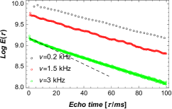
Figure 1: Spin echo decays of water at three modulation frequencies, presented by $N=40,300$ and $600$ echo peaks respectively, show a clear deviation from a mono-exponential decay at $\nu=3$kHz .

Complex spin dynamics under the influence of the sequence of RF pulses and various magnetic fields can be solved by using Feynman’s operator calculus  Feynman ; Dyson , in which the Hamiltonian is transformed into a series interaction representations. Subsequent transformations of system, into the frame of molecular motion with the disentanglement of ${\cal H}_{L}$ in Eq.2, then into the frame rotating with $\omega_{o}$ and finally into the toggling frame determined by ${\cal H}_{cpmg}^{y}(t)$  moj81 ; mojcall , amounts into the effective gradient/RF Hamiltonian moj16 , which describes a combined effect of RF and MFG fields as  moj16

$${\cal H}_{gt}(t)=-\sum_{i}{\omega_{z}({\mathbf{r}}_{i}(t))[{\cal I}_{zi}\cos{b(t)}-{\cal I}_{xi}\sin{b(t)}]}.$$ (3)

Here, $\omega_{z}({\mathbf{r}}_{i})$ is the $z$-component of ${\bf\omega}({\mathbf{r}}_{i})$, which includes the molecular motion, and the term with ${\cal I}_{xi}$, which describes the resonance off-set due to simultaneous application of MFG and RF-pulses. The first term of Eq.3 changes sign after each $\pi$-RF pulse, because $b(t)=\int_{0}^{t}{\omega_{\pi}(t^{\prime})dt^{\prime}}$ toggles $\cos{b(t)}$ between $\pm 1$. In the case of the infinitely short $\pi$-RF pulses, the fast transition between $\pm$-states allows us to neglect the second term, but not so if $\pi$-RF pulses have finite width $\delta$. Then a pulsed perturbation along ${\cal I}_{x}$ appears during the transitions. It can affect the MGSE measurement of molecular self-diffusion as shown in the Appendix.

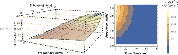
Figure 2: Frequency/temporal plots of ADC of water (left) and the variance $<D^{2}>$ (right) at 23^∘C. The variance levels to zero at long $\tau$ showing that the distribution of motional properties disappears, when the molecule trajectories are long enough to span the whole space of heterogeneity.

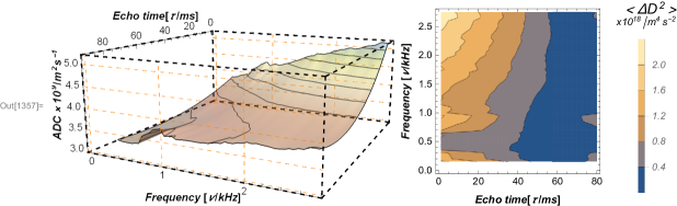
Figure 3: Frequency/temporal variation of ADC of toluene (left), and of variance $<D^{2}>$ (right) at 23 ^∘C.

In the case of $\pi$-RF pulses short enough that $\Delta\phi<1$ (see Appendix) and negligible spin relaxation, the first approximation of the spin echo amplitude induced by the $y$-component of magnetization at echo time $\tau=2NT$ is

$$E(\tau) \approx {d\over dt}\sum_{i}Tr\,\rho(\tau){\cal I}_{yi}$$ (4)

$$\approx \sum_{i}{\langle{\,\mathrm{e}^{\displaystyle{i\int_{0}^{\tau}\omega_{z}({\mathbf{r}}_{i}(t))\cos{b(t)}dt}}}\rangle},$$

if uniform sensitivity of the receiver coil across the excited volume of sample is assumed Ales09 . Here, the oscillation of $f(t)=\int_{0}^{t}\cos{(b(t^{\prime})}dt^{\prime}$ permits the integration par parts to write

$$E(\tau) \approx \sum_{i}{\langle{\,\mathrm{e}^{\displaystyle{-i\int_{0}^{\tau}\nabla\omega_{z}({\mathbf{r}}_{i}(t)\cdot{\mathbf{v}}_{i}(t)f(t)dt}}}\rangle},$$ (5)

where $\mathbf{v}_{i}(t)$ is the velocity of the tagged spin bearing particle at time $t$.

Generally, fluctuations of a molecular system in the thermal equilibrium are characterized by correlation functions of relevant physical quantities. Here, we assume that MFG is strong enough that only fluctuation of molecular translation velocity, $\Delta{\mathbf{v}}_{i}(t)={\mathbf{v}}_{i}(t)-\langle{{\mathbf{v}}_{i}(t)}\rangle$, can be taken into account. With the assumption that $\Delta{\mathbf{v}}_{i}(t)$ is a random variable, Eq.5 can be expanded into the cumulant series. In case when the spatial discord of spin phase created by MFG, i.e. $\lambda=2\pi/\gamma GT$, is larger than the spin displacements in the interval $T$, the first two terms of expansion are sufficient for the Gaussian phase approximation, which gives the spin echo amplitude moj81 ; mojcall ; moj202

$$E(\tau) = \sum_{i}E_{oi}\,\mathrm{e}^{\displaystyle{i\alpha_{i}(\tau)-\beta_{i}(\tau)}},$$ (6)

where the sum goes over the sub-ensemble of spins that have the same dynamical properties. In the case of molecular diffusion in homogeneous media, the first phase shift term

$$\alpha_{i}(\tau)=\int_{0}^{\tau}\nabla\omega_{z}({\mathbf{r}}_{i}(t))\cdot\langle{{\mathbf{v}}_{i}(t)}\rangle f(t)dt$$

is canceled after a few CPMG cycles due to toggling effect of $f(t)$. However, This is not true in the case of the restricted diffusion moj202 . The second term describes the echo attenuation, which can be expressed in the frequency domain as mojcall

$$\beta_{i}(\tau) = \frac{1}{\pi}\int_{0}^{\infty}\mathbf{q}(\omega,\tau)\mathbf{D}_{i}(\omega,\tau)\mathbf{q}^{*}(\omega,\tau)\,d\omega.$$ (7)

Here the spectrum of the spin phase discord ${\mathbf{q}}(\omega,t)=\nabla\omega_{z}({\mathbf{r}}_{i})f(\omega,t)$ is determined by $f(\omega,t)$, which is the frequency spectrum of $f(t)$ moj81 ; moj85 . $\mathbf{D}_{i}$ is the tensor of the VAS

$$\mathbf{D}_{i}(\omega,\tau)=\frac{1}{\pi}\int_{-\infty}^{\infty}\langle{\Delta\mathbf{v}_{i}(t)\otimes\Delta\mathbf{v}_{i}(0)}\rangle_{\tau}e^{\displaystyle{-i\omega t}}dt,$$ (8)

After, a few CPMG cycles, $(N>4)$ mojcall3 , the power spectrum of $f(t)$ can be approximated by

$$\left|{f(\omega,t)}\right|^{2} \approx 2\pi t\sum_{k=-\infty}^{\infty}{\left|{c_{k}}\right|^{2}\delta(\omega-k\omega_{m})},$$ (9)

in which narrow lobes with the amplitude
$\left|{c_{k}}\right|^{2}=4\sin{(k\pi/2)}^{2}/k^{4}\pi^{2}\omega_{m}^{2}$ appear at the multiples of the modulation frequency, $\omega_{m}=\pi/T$ . Neglecting all but the dominant first term and with MFG applied along the $z$-axis, the echo peak amplitude at $\tau=NT$ can be written as

$$E(\tau,\omega_{m}) = \sum_{i}{E_{oi}\,\mathrm{e}^{\displaystyle{-{\tau\over T_{2i}}-\frac{8\gamma^{2}G^{2}}{\pi^{2}\omega_{m}^{2}}D_{zzi}(\omega,\tau)\tau}}},$$ (10)

if spin relaxation is included. Here $D_{zzi}(\omega,\tau)$ is the $z$-projection of the VAS tensor averaged over the trajectories of molecular motion in the interval $\tau$. The described method provides the low frequency part of the VAS by changing the modulation frequency in the range, which is limited above by the power of RF transmitter.

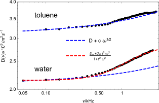
Figure 4: The VAS of water and toluene at 23 ^∘C obtained at $\tau>50$ ms, when the spin echo decays mono-exponentially. Red dashed lines show the fit by Eq.12, while the blue dashed lines show the fit by the anticipated $\sqrt{\omega}$-dependence of spectrum corresponding to $t^{-3/2}$-LTT dependence of VAF. It matches reasonably well only for VAS of toluene.

3 Experiments

Measurements were carried out on two different systems: TecMag $100$ MHz NMR spectrometer with a $2.35$ T superconducting magnet equipped with the Maxwell gradient coils capable of generating MFG in steps to $5.7$ T/m. Its high field allows precise MGSE measurement of VAS in liquids, but low MFG limits the frequency range to the interval from $50$ Hz to $3000$ Hz. Spin relaxation contribution is determined by separate measurements in zero MFG. Much higher but constant MFG of the NMR-MOUSE Blumich of $21.6$ T/m allows measurements in the frequency interval from $50$ Hz to $10$ kHz even of such slow self-diffusion as that of glycerol.

In order to test the effect of molecular interaction between nearest neighbors in dense fluid that could effectively hide the LTT Ryitsev ; McDonough ; Dib ; Bellissima , we conducted MGSE measurement on three polar liquids: distillate water, ethanol (analytical standard-Sigma-Aldrich), and glycerol (99.5$\%$-Sigma-Aldrich) with the dipole moments at room temperature of $1.85$ D, $1.69$ D, and $2.56$ D respectively and non-polar toluene (99.8 $\%$-Sigma-Aldrich). The interference of restriction to diffusion by sample boundaries was eliminated by enclosing the samples in a cylindrical glass cell, $15$ mm long and with $5$ mm diameter, which are much larger than molecular displacements in the interval of measurement.

The results were checked with the measurements of all samples on both systems, but with a lower accuracy on the NMR-MOUSE due its low proton Larmor frequency of $18.7$ MHz.

4 Results and discussion

Preliminary MGSE measurements of various liquids (water, ethanol, toluene, hexane, glycerol and water /glycerol mixtures) reveal unexpected low frequency features of VAS. Here we will only focus on the results of water, toluene, ethanol and glycerol. In each experiment a train of echoes was recorded with increasing $\tau$ (also $N$) and normalized for transverse relaxation. Experiments were repeated with different $T$ (thus changing the modulation frequency $\nu=1/2T$). Log of spin amplitude vs decay time $\tau$ is a line with the slope proportional to $D(\omega_{m})$ according to Eq.10. However, at short $\tau$ a nonlinear decay of attenuation is observed as shown in Fig.1. In a heterogeneous system, like liquid in porous medium, this is commonly attributed to the distribution of decay times. By grouping the spins into separate sub-ensembles corresponding to spins in different regimes of diffusion or in a different internal MFG moj16 one is able to distinguish groups of spins, which have differing starting points for their motion. In the case of short decay times $\tau$, the particle displacements are so small that their trajectories do not sample the entire space, and can convey information about heterogeneity of translational dynamics Swallen . The contribution of sub-ensembles with the distribution $P(D)$ to the recorded signal $E(\tau)=\int P(D)e^{-sD\tau}dD$ gives rise to non-exponential decay. With a small deviation from linearity the spin echo attenuation can be approximated by

$$\beta(\tau)=\log[E(\tau)]\approx-\tau/T_{2}-s\langle{D}\rangle\tau+\frac{s^{2}}{2}\langle{\Delta D^{2}}\rangle\tau^{2}+...,$$ (11)

where $\langle{D}\rangle$ is the mean diffusion coefficient, $\langle{\Delta D^{2}}\rangle$ is the variance of distribution and $s=\frac{8\gamma^{2}G^{2}}{\pi^{2}\omega^{2}}$ is given in Eq.10. Fitting the spin echo decays obtained by the measurements in water, toluene, and ethanol by the polynomial of the fifth order gives the curves with the coefficient of determination $R^{2}>0.999999$. After normalization for the spin relaxation time, first derivatives of $\beta(\tau)$ give the values, which we considered as ADCs. Their dependence on the spin-echo time $\tau$ and on the frequency of modulation $\nu=1/2T$ are presented in a frequency/temporal 3D plots in Fig.2 for water, and in Fig.3 for toluene. Both figures are supplemented by the frequency/temporal contour plot of second derivatives of $\beta(\tau)$, which describe the variance of diffusion distribution, $\langle{\Delta D^{2}}\rangle$. Figures show that at short $\tau$ and at high modulation frequencies there is a non-zero value of variance, which reflects local diversity observed when particle trajectories are short enough. Figures also show that at $\tau$ longer than $40$ ms and frequencies below $50$ Hz, when particle trajectories are long enough to span whole space of heterogeneity, $\langle{\Delta D^{2}}\rangle$ levels to zero and ADC becomes equal to VAS of the liquid. The same is shown for the ethanol in Fig.5. From the frequency dependence of $\langle{\Delta D^{2}}\rangle$, we can estimate the size of heterogeneity to about a few tens of micrometers, which agrees with predictions Mazur .

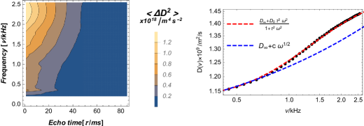
Figure 5: Frequency/temporal plots of the variance $<D^{2}>$ (left) and VAS of ethanol (right) at 23 ^∘C obtained from the spin echo attenuation in the range of mono-exponential decay. Red dashed line shows a good fit by Eq.12, but only a few points at the low frequencies can be approximately fitted with LTT-dependence (the blue dashed).

When molecules are packed together in liquids, the attractive/repulsive interactions between neighbors exert effects that could be reflected in the VAS of liquids as was already confirmed by the simulation studies Ryitsev ; McDonough ; Dib . In the case of polar liquids like water, ethanol, and glycerol impact of this interactions on the VAS should be much greater than for a non-polar toluene The results of measurement in toluene, shown in Fig.3, exhibit a non-exponential decay at short $\tau$, but data obtained from the interval of mono-exponential decay ( $\tau>40$ ms) give the VAS of toluene, changing from $3.60\times 10^{-9}$ m²/s at $40$ Hz to $4.45\times 10^{-9}$ m²/s at $3$ kHz. The anticipated $\sqrt{\omega}$-dependence, corresponding to $t^{-3/2}$-LTT of VAF, can be roughly fitted to the obtained the VAS of toluene with the deviation within the experimental error, as shown in Fig.4. While the VAS of water, obtained in the interval of mono-exponential decay, which increases from $2.2\times 10^{-9}$ m²/s at $50$ Hz to $2.75\times 10^{-9}$ m²/s at $3$ kHz, and the same of ethanol, which increases from $1.15\times 10^{-9}$ m²/s at $40$ Hz to $1.45\times 10^{-9}$ m²/s at $3$ kHz, show strong deviation from $\sqrt{\omega}$ as shown on Figs.4 and 5. These figures show attempts to fit initial few points in the frequency range below $500$ Hz for water and below $900$ Hz for ethanol with $\sqrt{\omega}$-curve, which show a strong deviation from experimental data at higher frequencies..

Self-diffusion coefficients in these liquids mostly follow the Arrhenius law DouglassVFC , which means that the molecules in liquid state are momentarily trapped in potential wells created by their neighbors. These measurements gave an averaged excitation potential for water of $18$ kJ/mol while for non-polar toluene of about $8$ kJ/mol. We assume that molecular motions and hydrodynamic fluctuations reduce the potential well enough to allow approximation of the molecular dynamics with the set of Langevin equations of particles harmonically coupled in pairs. Its solution gives the low frequency part of VAS in the form

$$D_{c}(\omega)=\frac{D_{\infty}+D_{o}\tau_{c}^{2}\omega^{2}}{1+\tau_{c}^{2}\omega^{2}},$$ (12)

if the inertial terms are neglected. Here, $D_{\infty}$ is an averaged diffusion rate, which depends on the number of coupled molecules, and $D_{o}$ is the diffusion rate of a molecule escaping the binding. $\tau_{c}$ is the correlation time, which shortens with the strength of binding. Fig.4 and Fig.5 show fits of $D_{c}$ from Eq.12 to the obtained data for VAS of water and ethanol with the coefficient of determination of $R^{2}>0.99994$.

NMR MOUSE, device with a strong constant MFG and low Larmor frequency $\omega_{o}$, is not suitable for the measurements of water, ethanol and toluene below $1$ kHz, because of excessive attenuation at low frequencies, i.e. at long $T$. Nevertheless, their VAS at higher frequencies match well those from $100$ MHz NMR spectrometer. But the strong MFG of NMR MOUSE suits well for the measurement of very low diffusion coefficient of glycerol, a substance with large dipole moment and strong hydrogen bondings. The inset in Fig.6 shows that ADC of glycerol does not exhibit any dependence on the echo times. This means that unlike water and alcohol, there is no effect of distribution of diffusion on evolution times. It allows a direct exponential fitting of its echo decays providing the VAS of glycerol with the coefficient of determination of $R^{2}\approx 0.9996$ as shown in Fig.6. It changes from the initial value of $3\times 10^{-13}$ m²/s at $50$ Hz to $10^{-9}$ m²/s at $10$ kHz. The data can be fitted by Eq.12, but with a lower coefficient of determination as shown in Tab.1.

The asymptotic values of VAS shown in Figs.4, 5 and 6 to the zero frequency, which are equal to the diffusion coefficient in accordance with the Einstein’s definition in Eq.1, for all liquids, correspond to the values obtained from measurements on other devices Mills ; Pickup ; Meckl ; DErrico .

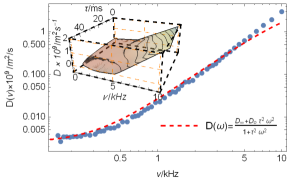
Figure 6: VAS of glycerol at 23 ^∘C obtained by NMR MOUSE fits well with the formula 12 (red dashed line), while 3D inset shows the absence of temporal variation.

Table 1: Parameters of Eq.12 fitting to VAS

sample	$D_{\infty}$	$D_{o}/10^{-9}$ m2s-1	$\tau_{c}$/ms	$R^{2}$
Ethanol	$1.12$	$1.54$	$0.11$	$0.99996$
Water	$2.19$	$2.9$	$0.12$	$0.99996$
Glycerol	$0.0025$	$5$	$0.01$	$0.940$

5 Conclusion

In conclusion we can state that MGSE measurements unveil the low frequency VAS of simple liquids, which approximately endorse the LTT origin predicted by the theory and simulations only for toluene, while in the cases of ethanol, water and glycerol, low-frequency VAS can be better explained by self-diffusion of molecules temporarily trapped in potential wells created by their neighbors in their course of motion. Even in the case of toluene, the deviation from the LTT dependence that is within the experimental error could be attributed to interactions, which are small compared to polar fluids, which also is proven by the smallness of its diffusive excitation potential of $8$ kJ/mol.

Spin-echo non-exponential decay in the initial short time intervals, unambiguously confirms an existence of diversity of diffusion in bulk of liquids, which is not for instance the consequence of media in-homogeneity as observed in the diffusion measurement in the porous system. Given that the method provides the ensemble average of VAS over the particle trajectories in the time interval of measurement, the transition into mono-exponential spin-echo decay at longer times means that long enough trajectories, which traverse entire space of in-homogeneity, conveys VAS averaged over the space of heterogeneity.

The inset in Fig.6 shows that ADC of glycerol does not exhibit any dependence on echo times. We speculate that the observed the variance of diffusion distribution in the bulk of liquids is associated with hydrodynamic fluctuations, in which the molecular diffusion process is affected by the vortex motion of fluid Alder2 . Thus, in addition to the size of heterogeneity, the rate of its change is also important. Thus, we can explain the absence of $\langle{\Delta D^{2}}\rangle$ in the glycerol by the fluctuation of hydrodynamic vortexes, with rate too fast to be observed in the shortest intervals $T$ attainable by our devices. According to the derivation of Eq.12, a shorter $\tau_{c}$ means also stronger interactions. Tab.1 shows the correlation times, among which $\tau_{c}$ of glycerol is ten times shorter than those of water and ethanol, which corresponds to the magnitude of dipole moment of these liquids.

So we can conclude that MGSE measurements provide information of molecular translation dynamics in liquids, which can be explained as a combination of molecular self-diffusion and eddy diffusion processes Graham in the vortexes of hydrodynamic fluctuation, while LTT is effectively hidden by intermolecular interactions in polar liquids.

6 Acknowledgement

We acknowledge the contribution of prof. dr. Igor Serša and dr. Franci Bajd from Josef Stefan Institute to assist in the preparation of experiments and Slovenian research agency, ARRS, for the financial support in the program P1-0060.

7 Appendix

Given that ${\cal H}_{gt}(t)$ is periodic and cyclic with period $2T$, the resonance off-set effect can be calculated by using the Magnus expansion of the time evolution operator Magnus . The expansion to the third order of the cumulant series gives the averaged Hamiltonian, whose first term has been already considered in Sec.2.1. The derivation of the second and the third terms results in the Hamiltonian

$${\cal H}_{gtc}=-(1-\delta/2T)\frac{\delta}{\pi}\sum_{i}{\omega({\mathbf{r}}_{i})^{2}[{\cal I}_{yi}-\frac{\delta}{\pi}\omega({\mathbf{r}}_{i}){\cal I}_{zi}]},$$ (13)

which describes the resonance off-set distortion over a cycle $2T$ as an additional spin rotation in the interval of $\pi$-RF pulse application. Straightforward calculation results in a factor effecting the signal induced by the $y$-component of the $i$-th spin sub-ensemble as

$$k_{ic}=\frac{1+\Delta\phi_{i}^{2}\cos\left(\pi\tau(1-\delta/2T)\Delta\phi_{i}^{2}\sqrt{1+\Delta\phi_{i}^{2}}/\delta\right)}{1+\Delta\phi_{i}^{2}},$$ (14)

where $\Delta\phi_{i}=\frac{\delta}{\pi}\omega({\mathbf{r}}_{i})$. Summation over the sub-ensembles in the volume, which is either selected by the initial $\pi/2$-RF pulse excitation in the background of MFG or determined by the size of the sample container moj16 , gives the reduction factor of the echo amplitude

$$k_{c}=\frac{2}{\Delta\phi}\arctan{\Delta\phi/2}$$ (15)

with $\Delta\phi=\frac{\delta}{\pi}\gamma\left|{{\mathbf{G}}\cdot\Delta{\mathbf{r}}}\right|$, where $\left|{\Delta{\mathbf{r}}}\right|$ is the width of the excited spin slice. Added to the signal is also a small oscillation with the amplitude ${\Delta\phi}^{2}/12$ and the frequency ${\Delta\phi}^{2}/2\delta$ as shown in Fig.1. Therefore, the interval of observed echo decay should be much longer than the inverse frequency of oscillations, $\tau>2\delta/{\Delta\phi}^{2}$ in order to obtain correct information about molecular motion from the average over the signal oscillations. The spin excitation by initial $\pi/2$-RF pulse in the background of constant MFG provides the active volume giving ${\Delta\phi}\approx 1$, which means that averaging over the time of several $\delta$ is sufficient to suppress resonance off-set distortion.

At the end of this discussion, it is necessary to address the description of the spin echo by the concept of coherence pathways, which is sometimes incorrectly used in MGSE measurements. Accordingly, the contributions of different coherence pathways to the shape and decay of signal differently depend on diffusion and relaxation Hurlimann2 ; YQSong ; Toumelin . By the frequency filtering of the spin echo signal certain coherence pathways can be excluded so that we get the one that best suits the diffusion and relaxation measurements. The zero frequency filtered echo signal, which isolates the direct coherence pathway, is considered as the best to provide credible information about molecular diffusion. This is true if we assume the self-diffusion coefficient which is constant in the interval of measurement. In the case of a slow molecular motion, the signal filtering removes information about motion that is above the threshold frequency of low pass filter as is proven by measurements of water in the reference Sersa . Thus, the straightforward calculation of the time integral over the spin echo is by definition the zero frequency component spin echo, in which all information about the spin motion with frequencies $\omega_{c}>\gamma\left|{{\mathbf{G}}\cdot\Delta{\mathbf{r}}}\right|/2$ are filtered out. Thus, it is important to take into account the principle of diffusion measurement by the gradient spin echo, where only the peak of the spin echo, which is by definition the integral over the whole echo spectrum, $E(N\tau)=\int E(\omega)d\omega$, conveys information about molecular translational motions Stejskal651 ; moj81 ; mojcall , while the Fourier transformation of the spin echo signal gives the image of the spin spatial distribution. This is similar to the uncertainty principle in the quantum mechanics: “The more precisely the position of a particle is given, the less precisely can one say what its momentum is.”.

8 Authors contributions

J. Stepišnik, C. Mattea and A. Mohorič were involved in the measurements and the preparation of the manuscript, while S. Stapf has read and approved the final manuscript.

References

- (1) L.D. Landau, E.M. Lifshitz, J. Exp. Theoret. Phys. 32, 618 (1957)
- (2) V. Vladimirsky, J. Terletzky, J. Exp. Theoret. Phys. 15, 258 (1945)
- (3) M.S. Giterman, M.E. Gertsenshtein, J. Exp. Theoret. Phys. 23, 723 (1966)
- (4) L. Landau, E. Lifshitz, Fluid Mechanics ( Volume 6 of A Course of Theoretical Physics ) (Pergamon Press, Oxford, 1959)
- (5) B. Alder, T. Wainwright, Phys. Rev. Lett. 18, 988 (1967)
- (6) B. Alder, T. Wainwright, Phys. Rev. A 1, 18 (1970)
- (7) M. Sakamoto, J. Phys. Soc. Japan 19, 1862 (1964)
- (8) K.F. Larsson, Phys. Rev.. 167, 171 (1968)
- (9) V. Ardente, G. Nardelli, L. Reatto, Physical Review 148, 124 (1966)
- (10) G. Maret, P. Wolf, Z. Phys. B 65, 409 (1987)
- (11) J.P. Boon, S. Yip, Molecular hydrodynamics (Dover Publications, Incorporated, New York, 2013)
- (12) J. Boon, A. Bouller, Phys. Letters A 55, 391 (1976)
- (13) G.L. Paul, P.N. Pusey, J. Physics A: Math. and general. 14, 3301 (1981)
- (14) W. van Megen, Phys. Rev. E 73, 011401 (2006)
- (15) W.K. Kegel, A. van Blaaderen, Science 287, 290 (2000)
- (16) J.R. Dorfman, E.G.D. Cohen, Phys. Rev. A 12, 292 (1975)
- (17) D. Levesque, L. Verlet, Phys. Rev. A 2, 2514 (1970)
- (18) D. Levesque, T. Ashurst, Phys. Rev. Lett. 33, 277 (1974)
- (19) J. Marro, J. Masoliver, Phys. Rev. Lett. 54, 731 (1984)
- (20) A. Rahman, Phys. Rev. 136, A 405 (1964)
- (21) C.D. Andriesse, Physica 48, 61 (1970)
- (22) K. Carneiro, Phys. Rev. A 14, 517 (1976)
- (23) C. Morkel, C. Gronemeyer, W. Glaser, J. Bosse, Phys. Rev. Lett. 58, 1873 (1987)
- (24) H.L. Peng, H.R. Schober, T. Voigtmann, Phys. Rev. E 94, 060601(R) (2016)
- (25) R.E. Ryitsev, N.M. Chtchelkatchev, J. Chem. Phys 141, 124509 (2014)
- (26) A. McDonough, S.P. Russo, I.K. Snook, Phys. Rev. E 63, 026109 (2011)
- (27) R.F.A. Dib, F. Ould-Kaddour, Phys. Rev. E 74, 011202 (2006)
- (28) S. Bellissima, M. Neumann, E. Guarini, U. Bale, F. Barocchi, Phys. Rev. E 92, 042166 (2015)
- (29) J. Stepišnik, A. Mohorič, C. Matea, S. Stapf, I. Serša, EuroPhysics Letters 106, 27007 (2014)
- (30) S. Lasič, J. Stepišnik, A. Mohorič, I. Serša, G. Planinšič, Europhysics Letters 75, 887 (2006)
- (31) J. Stepišnik, P. Callaghan, Physica B 292, 296 (2000)
- (32) P.T. Callaghan, S.L. Codd, Phys. of fluids 13, 421 (2001)
- (33) D. Topgaard, C. Malmborg, O. Soederman, J. Mag. Res. 156, 195 (2002)
- (34) E.C. Parsons, M.D. Does, J.C. Gore, Magn. Reson. Imaging 21, 279 (2003)
- (35) R. Mills, J. Phys. Chem. 77, 685 (1973)
- (36) E.L. Hahn, Phys. Rev. 80, 580 (1950)
- (37) H.Y. Carr, E.M. Purcell, Phys. Rev. 94, 630 (1954)
- (38) H.C. Torrey, Phys. Rev. 104, 563 (1956)
- (39) E.O. Stejskal, J. Chem. Phys 43, 3597 (1965)
- (40) N. Galamba, J. Phys.: Condens. Matter 29, 015101 (2017)
- (41) F. Mallamace, M. Broccio, C. Corsaro, A. Faraone, L. Liu, C.Y. Mou, S.H. Chen, J. Phys.: Condens. Matter 18, S2285–2297 (2006)
- (42) R. Lamanna, M. Delmelle, S. Cannistraro, Physical Review E 49, 2841 (1994)
- (43) A. Chandra, S. Chowdhuri, Proc. Indian Acad. Sci. 113, 591 (2001)
- (44) M. Mahoney, W. Jorgensen, J. Chem. Phys. 114, 363 (2001)
- (45) K. Krynicki, C.D. Green, , D.W. Sawyer, Faraday Discuss. Chem. Soc. 66, 199 (1978)
- (46) K. Yoshida, C. Waka, N. Matubayasi, M. Nakahara, J. Chem. Phys. 123, 164506 (2005)
- (47) A. Einstein, Annalen der Physik 322, 891 (1905)
- (48) R. Kubo, Rep. Prog. Phys. 29, 255 (1966)
- (49) W.M. Visscher, Phys. Rev. A 7, 1439 (1973)
- (50) V. Lisy, J. Tothova, J. Mol. Liquids 234, 182 (2017)
- (51) J. Stepišnik, Physica B 104, 350 (1981)
- (52) J. Stepišnik, Prog. Nucl. Magn. Reson. Spectrosc. 17, 187 (1985)
- (53) P. Callaghan, J. Stepišnik, J. Magn. Reson. A 117, 118 (1995)
- (54) P. Callaghan, J. Stepišnik, Advances in Magnetic and Optical Resonance, ed.Warren S. Warren (Academic Press, Inc, San Diego, 1996), Vol. 19, chap. Generalised Analysis of Motion Using Magnetic Field Gradients, pp. 326–89
- (55) M. Aggarwal, M. Jones, P. Calabresi, S. Mori, J. Zhang, Magnetic resonance in medicine 67, 98 (2012)
- (56) J. Stepišnik, I. Ardelean, J. Magn. Reson. 272, 100 (2016)
- (57) S. Meiboom, D. Gill, Rev. Sci. Inst.. 29, 688 (1958)
- (58) J. Kowalewski, L. Maler., Nuclear spin relaxation in liquids : theory, experiments, and applications (Series in chemical physics, Taylor and Francis Group, 6000 Broken Sound Parkway NW, Suite, 2006)
- (59) R.P. Feynman, Phys. Rev. 84, 109 (1951)
- (60) F. Dyson, Phys. Rev. 75, 486 (1949)
- (61) A. Mohorič, J. Stepišnik, Prog. Nucl. Magn. Reson. Spectrosc. 54, 166 (2009)
- (62) J. Stepišnik, Europhysics Letters 60, 453 (2002)
- (63) B. Bluemich, F. Casanova, S. Appelt, Chem. Phys. Letters. 477, 231 (2009)
- (64) S.F. Swallen, P.A. Bonvallet, R.J. McMahon, M.D. Ediger, Phys. Rev. Lett. 90, 015901 (2003)
- (65) P. Mazur, G. van der Zwan, Physica A: Statistical Mechanics and its Application 92, 483 (1978)
- (66) D.C. Douglass, J. Chem. Phys. 35, 81 (1961)
- (67) S. Pickup, F. Blum, Macromolecules 22, 3961 (1989)
- (68) S. Meckl, M. Zeidler, Mol. Phys 63, 85 (1988)
- (69) G. D’Errico, O. Ortona, F. Capuano, V. Vitagliano, J. of Chem. Eng. Data 49, 1665 (2004)
- (70) D.I. Graham, Int. J. of Multiphase Flow 27, 1065 (2001)
- (71) W. Magnus, Commun. Pure Appl. Math. 7, 649 (1954)
- (72) M.D. Hurlimann, J. Mag. Res 148, 367–378 (2001)
- (73) Y.Q. Song, J. Magn. Reson. 157, 82–91 (2002)
- (74) E. Toumelin, C. Torres-Verdın, B. Sun, K. Dunn, J. of Mag. Res. 188, 83–96 (2007)
- (75) I. Serša, F. Bajd, A. Mohorič, J. Mag. Res. 270, 77 (2016)
- (76) E.O. Stejskal, J.E. Tanner, J. Chem. Phys. 42, 288 (1965)