The grand canonical ABC model: a reflection asymmetric mean field Potts model

Abstract

We investigate the phase diagram of a three-component system of particles on a one-dimensional filled lattice, or equivalently of a one-dimensional three-state Potts model, with reflection asymmetric mean field interactions. The three types of particles are designated as $A$, $B$, and $C$. The system is described by a grand canonical ensemble with temperature $T$ and chemical potentials $T\lambda_{A}$, $T\lambda_{B}$, and $T\lambda_{C}$. We find that for $\lambda_{A}=\lambda_{B}=\lambda_{C}$ the system undergoes a phase transition from a uniform density to a continuum of phases at a critical temperature $\hat{T}_{c}=(2\pi/\sqrt{3})^{-1}$. For other values of the chemical potentials the system has a unique equilibrium state. As is the case for the canonical ensemble for this $ABC$ model, the grand canonical ensemble is the stationary measure satisfying detailed balance for a natural dynamics. We note that $\hat{T}_{c}=3T_{c}$, where $T_{c}$ is the critical temperature for a similar transition in the canonical ensemble at fixed equal densities $r_{A}=r_{B}=r_{C}=1/3$.

Keywords: ABC model, grand canonical ensemble, reflection asymmetric mean field three-state Potts model

1 Introduction

In this paper we study the phase diagram of the three species ABC model on an interval as a function of the chemical potentials and the temperature. The system is defined microscopically on a lattice of $N$ sites in which each site is occupied by either an $A$, a $B$, or a $C$ particle. The energy is of mean field type, with an interaction which has cyclic symmetry in the particle types but is reflection asymmetric:

$$E_{N}({\underline{\zeta}})={\frac{1}{N}}\sum^{N-1}_{i=1}\sum^{N}_{j=i+1}[\eta_{C}(i)\eta_{B}(j)+\eta_{A}(i)\eta_{C}(j)+\eta_{B}(i)\eta_{A}(j)].$$ (1.1)

Here the configuration ${\underline{\zeta}}$ of the model is an $N$-tuple $(\zeta_{1},\ldots,\zeta_{N})$, with $\zeta_{i}=A$, $B$, or $C$, and $\eta_{\alpha}(i)$, $\alpha=A,B,C$, is a random variable which specifies whether a particle of species $\alpha$ is present at site $i$: $\eta_{\alpha}(i)=1$ if $\zeta_{i}=\alpha$ and $\eta_{\alpha}(i)=0$ otherwise, so that always $\sum_{\alpha}\eta_{i}(\alpha)=1$.

We remark that we may also regard the model as a reflection asymmetric mean field three state Potts model. The asymmetry of the interaction, however, gives this model system very different behavior from that of the usual symmetric mean field model [1]. Similar but short-range (in fact, nearest neighbor) reflection asymmetric interactions occur in chiral clock models [2, 3, 4]; see Remark 5.1 below.

The equilibrium probability of a configuration ${\underline{\zeta}}$ is given by the grand canonical Gibbs measure

$$\mu_{\beta,\lambda}({\underline{\zeta}})=\Xi^{-1}\exp[-\beta E_{N}({\underline{\zeta}})+\sum_{\alpha}\lambda_{\alpha}N_{\alpha}(\zeta)],$$ (1.2)

where $\beta$ is the inverse temperature, $\lambda_{A}$, $\lambda_{B}$, and $\lambda_{C}$ are $\beta$ times the chemical potentials, $N_{\alpha}=\sum^{N}_{i=1}\eta_{\alpha}(i)$ with $\sum_{\alpha}N_{\alpha}=N$, and $\Xi$ is the usual grand canonical partition function. We prove here that in the scaling limit ($N\to\infty$, $i/N\to x\in[0,1]$) the equilibrium density profiles $\rho(x)$ are unique and spatially nonuniform when the $\lambda_{\alpha}$’s are not all the same. When $\lambda_{A}=\lambda_{B}=\lambda_{C}$ the densities are spatially uniform above a critical temperature $\hat{T}_{c}=\hat{\beta}_{c}^{-1}$, with $\hat{\beta}_{c}=2\pi/\sqrt{3}$; below $\hat{T}_{c}$ the profiles have a natural extension to periodic functions with a period three times the length of the system.

One may compare the behavior described above with that of the same system in the canonical ensemble, in which the $N_{\alpha}$ are taken as fixed; this is the only case considered previously. The results are quite different, that is, we have inequivalence of ensembles (see [5, 6] for recent reviews). We give in Section 2 a brief history of the ABC model with fixed particle number and a summary of results for that system. In Section 3 we describe a stochastic evolution satisfying detailed balance with respect to the measures $\mu_{\beta,\lambda}({\underline{\zeta}})$, and in Section 4 we establish the phase diagram. Section 5 gives a discussion of some related models and problems.

2 The ABC model in the canonical ensemble

The ABC model was introduced by Evans et al. [7] (see also [8, 9, 10, 11, 12, 13, 14]) as a one dimensional system consisting of three species of particles, labeled $A,B,C$, on a ring containing $N$ lattice sites; we will typically let $\alpha=A$, $B$, or $C$ denote a particle type, and make the convention that $\alpha+1$, $\alpha+2$, $\ldots$ denote the particle types which are successors to $\alpha$ in the cyclic order $ABC$. The system evolves by nearest neighbor exchanges with asymmetric rates: if sites $i$ and $i+1$ are occupied by particles of different types $\alpha$ and $\gamma$, respectively, then the exchange $\alpha\,\gamma\to\gamma\,\alpha$ occurs at rate $q<1$ if $\gamma=\alpha+1$ and at rate $1$ if $\gamma=\alpha-1$. The total numbers $N_{\alpha}$ of particles of each species are conserved and satisfy $\sum_{\alpha}N_{\alpha}=N$. In the limit $N\to\infty$ with $N_{\alpha}/N\to r_{\alpha}$, where $r_{\alpha}>0$ for all $\alpha$, the system segregates into pure $A$, $B$, and $C$ regions, with rotationally invariant distribution of the phase boundaries.

In the weakly asymmetric version of the system introduced by Clincy et al. [9], in which $q=e^{-\beta/N}$, the stationary state for the equal density case $N_{A}=N_{B}=N_{C}$ is a Gibbs measure of the form $\exp\{-\beta E_{N}\}$, so that the parameter $\beta=T^{-1}$ plays the role of an inverse temperature. The energy $E_{N}$ is given by (1.1), and the condition $N_{A}=N_{B}=N_{C}$ ensures that this is translation invariant, despite the appearance of a preferred starting site for the summations.

Ayyer et. al. [14] studied the weakly asymmetric system on an interval, that is, again on a one-dimensional lattice of $N$ sites but now with zero flux boundary conditions, so that a particle at site $i=1$ (respectively $i=N$) can only jump to the right (respectively left). For this system the steady state is always Gibbsian, given by $\exp\{-\beta E_{N}\}$ with $E_{N}$ as in (1.1), whatever the values of $N_{A}$, $N_{B}$, and $N_{C}$. When $N_{A}=N_{B}=N_{C}$ the steady state of the system thus agrees with that on the ring, so that the invariance under rotations on the ring then implies a rather surprising “rotation” invariance of the Gibbs state on the interval. We describe the results of [14] in some detail, since the work of the current paper depends heavily on them.

To identify typical coarse-grained density profiles at large $N$, [14] considers the scaling limit

$$N\to\infty,\qquad i/N\to x,\quad x\in[0,1].$$ (2.1)

For this limit there exists a Helmholtz free energy functional $\beta^{-1}{\cal F}(\{n\})$ of the density profile $n(x)=(n_{A}(x),n_{B}(x),n_{C}(x))$. ${\cal F}$ is the difference of contributions from the energy and entropy:

$${\cal F}(\{n\})=\beta{\mathcal{E}}(\{n\})-{\mathcal{S}}(\{n\}),$$ (2.2)

where ${\mathcal{E}}\left(\{n\}\right)$ and ${\mathcal{S}}\left(\{n\}\right)$ are the limiting values of the energy and entropy per site:

$${\mathcal{E}}\left(\{n\}\right) = \int_{0}^{1}\,dx\int_{x}^{1}\,dz\sum_{\alpha}n_{\alpha}(x)n_{\alpha+2}(z),$$ (2.3)

$${\mathcal{S}}(\{n\}) = -\int_{0}^{1}dx\sum_{\alpha}n_{\alpha}(x)\ln n_{\alpha}(x).$$ (2.4)

We will write ${\cal F}={\cal F}^{(\beta)}$ when we need to indicate explicitly the $\beta$ dependence. Only the canonical ensemble was considered in [14], so that for some fixed positive mean densities $r_{A}$, $r_{B}$, $r_{C}$ satisfying $r_{A}+r_{B}+r_{C}=1$ the profiles $n(x)$ in (2.2)–(2.4) satisfy the conditions

$$0\leq n_{\alpha}(x)\leq 1,\quad\sum_{\alpha}n_{\alpha}(x)=1,\quad\hbox{and}\quad\int^{1}_{0}n_{\alpha}(x)dx=r_{\alpha}.$$ (2.5)

The typical profiles in the scaling limit are those which minimize ${\cal F}$; it was shown in [14] that such minimizers always exist and satisfy the ELE derived from ${\cal F}$. To obtain the ELE one defines

$${\cal F}_{\alpha}(x) =\frac{\delta{\cal F}}{\delta n_{\alpha}(x)}$$

$$=\log n_{\alpha}(x)+\beta\int_{0}^{x}[n_{\alpha+1}(z)-n_{\alpha+2}(z)]\,dz+1+\beta r_{\alpha+2}$$ (2.6)

to be the variational derivative taken as if the profiles $n_{A}(x)$, $n_{B}(x)$, and $n_{C}(x)$ were independent; the constraints (2.5) then imply that at a stationary point of ${\cal F}$ both ${\cal F}_{A}-{\cal F}_{C}$ and ${\cal F}_{B}-{\cal F}_{C}$ are constant. After simple manipulations (see also Section 4 below) this yields the ELE satisfied by the typical profiles $\rho(x)$:

$$\frac{d\rho_{\alpha}}{dx}=\beta\rho_{\alpha}(\rho_{\alpha-1}-\rho_{\alpha+1}),\qquad\alpha=A,B,C.$$ (2.7)

These are to be solved subject to (2.5) (written in terms of $\rho$ rather than $n$).

It follows from (2.7) that all relevant solutions satisfy $\prod_{\alpha}\rho_{\alpha}(x)=K$ for some constant $K$ with $0<K\leq 1/27$. For $K=1/27$ they are constant, with value $1/3$; for $K<1/27$ they have the form

$$\rho_{\alpha}(x)=y_{K}(2\beta(x-1/2)+t_{\alpha}),\qquad 0\leq x\leq 1,$$ (2.8)

with $y_{K}(t)$ a solution, periodic with period $\tau_{K}$, of the equation

$$\frac{1}{2}{y^{\prime}}^{2}+\frac{1}{2}Ky-\frac{1}{8}y^{2}(1-y)^{2}=0;$$ (2.9)

here $t=2\beta x+\rm constant$. $y_{K}$ is uniquely specified by requiring that it take on its minimum value at the points $t=n\tau_{K}$, $n\in{\mathbb{Z}}$. The phase shifts $t_{\alpha}$ in (2.8) satisfy

$$t_{A}=t_{B}+\tau_{K}/3\qquad\hbox{and}\qquad t_{C}=t_{B}-\tau_{K}/3.$$ (2.10)

Remark 2.1.

Equation (2.9) describes a particle of unit mass and zero energy oscillating in a potential $U_{K}(y)=Ky/2-y^{2}(1-y)^{2}/8$. The constant solution $y=1/3$ appears for $K=1/27$. For $K<1/27$, $y_{K}(t)$ is an even function which is strictly increasing on the interval $[0,\tau_{K}/2]$; it was shown in [14] that $\tau_{K}$ is a strictly decreasing function of $K$. Because the potential is quartic in $y$ the solution is an elliptic function. Further properties of the function $y_{K}$ are summarized in Proposition A.1 of Appendix A.

Equation (2.8) indicates that nonconstant solutions of the ELE are obtained by viewing $y_{K}(t)$, and its translates by one-third and two-thirds of a period, in some “window” of length $2\beta$. If one is given $\beta$ and $r=(r_{A},r_{B},r_{C})$ then one must determine $K$ and one of the phase shifts, say $t_{B}$, so that

$$r_{\alpha}=\frac{1}{2\beta}\int_{-\beta}^{\beta}y_{K}(t+t_{\alpha})\,dt,\qquad\alpha=A,B,C.$$ (2.11)

The solutions which minimize ${\cal F}$ were completely determined in [14]. In stating the result, we use the following terminology: a solution is of type $n$ if $(n-1)\tau_{K}<2\beta\leq n\tau_{K}$, that is, if the window contains more than $n-1$ and at most $n$ periods of the function $y_{K}$.

Theorem 2.2.

Suppose that $r_{A}$, $r_{B}$, and $r_{C}$ are strictly positive. Then:

(a) If $r_{A}=r_{B}=r_{C}=1/3$ then for the equations (2.7) with (2.5) there exist (i) the constant solution, (ii) for $\beta>n\beta_{c}=2\pi n\sqrt{3}$, $n=1,2,\ldots$, a family of solutions, of period $\tau_{K}=2\beta/n$ and hence of type $n$, differing by translation, and (iii) no other solutions. The minimizers of the free energy are, for $\beta\leq\beta_{c}$, the (unique) constant solution and, for $\beta>\beta_{c}$, any type 1 solution.

(b) For values of $r$ other than $(1/3,1/3,1/3)$ there exists for all $\beta$ a unique type 1 solution of these equations which is a minimizer of the free energy.

(c) At zero temperature ($\beta\to\infty$) the system segregates into either three or four blocks, each containing particles of only one type.

3 Dynamics of the grand canonical ABC model

We now turn to consideration of the ABC model on the interval when the number of particles can fluctuate; we will abbreviate this as the GCABC model. In Section 1 the corresponding grand canonical measure $\mu_{\beta,\lambda}$ (see (1.2)) was presented in the equilibrium setting as a Gibbs measure obtained from the energy function (1.1) and chemical potentials $\beta^{-1}\lambda_{\alpha}$. Just as for the canonical Gibbs measure, however, one may alternatively view this as the stationary measure for some dynamics; we describe two possibilities here. (A different generalization of the ABC model to a nonconserving dynamics, in which the system is on a ring, vacancies are permitted, and the total number of particles fluctuates but the differences $N_{\alpha}-N_{\gamma}$ are conserved, is given in [15, 16]. When all the $N_{\alpha}$ are equal the stationary measure has the form of a grand canonical ensemble.)

In the first dynamics we consider there are particle exchanges between adjacent sites, with the same rates as for the canonical dynamics. To allow the number of particles to fluctuate, however, we introduce two new possible transitions. First, if the particle at site $i=1$ is of type $\alpha$ then with a rate equal to $Ce^{-\lambda_{\alpha}}$ the entire configuration is translated by one site to the left, the particle at site $i=1$ disappears, and a particle of species $\alpha+1$ is created at site $i=N$. Second, with a rate equal to $Ce^{-\lambda_{\alpha+1}}$ the reverse transition occurs. Here $C$ is a constant which we shall in the future take equal to 1. This dynamics satisfies the detailed balance condition with respect to the Gibbs measure (1.2): if a transition ${\underline{\zeta}}\to{\underline{\zeta}}^{\prime}$ arises from an exchange of particles the argument is as for the canonical model [14], while if it comes from a transition of the new type, say in the “forward” direction as described above, then $E_{N}({\underline{\zeta}})=E_{N}({\underline{\zeta}}^{\prime})$ but $N_{\alpha}$ decreases by 1 and $N_{\alpha+1}$ increases by 1, and the detailed balance condition $e^{-\lambda_{\alpha}}\nu_{\beta}({\underline{\zeta}})=e^{-\lambda_{\alpha+1}}\nu_{\beta}({\underline{\zeta}}^{\prime})$ follows.

Remark 3.1.

One may also obtain this dynamics by considering a ring of $N$ sites, with each site occupied by an $A$, $B$, or $C$ particle and with a marker located on one of the bonds between adjacent sites. Adjacent particles exchange across any unmarked bond with the usual ABC rates, while the marker may move one bond to its left or right, and in doing so it changes the species of the particle it passes: with —$\times\,$ and — denoting a marked and unmarked bond, respectively, the transition $\hbox{---}\hbox to0.0pt{\hss$\times\,$}\ \alpha\ \hbox{---}\ \to\hbox{---}\ (\alpha+1)\ \hbox{---}\hbox to0.0pt{\hss$\times\,$}\$ occurs with a rate equal to $e^{-\lambda_{\alpha}}$ and the reverse transition with a rate equal to $e^{-\lambda_{\alpha+1}}$. If one then obtains a configuration on the interval from a ring configuration by letting the marked bond identify the boundaries of the interval—effectively by cutting the ring at the marked bond—one sees easily that the inherited dynamics on the interval is precisely the dynamics discussed above. A slight variation of this idea was mentioned in [14].

We define the second dynamics only for the case in which all the $\lambda_{\alpha}$ are equal. We obtain it by first defining a dynamics for the constrained ring: a ring of $3N$ sites populated by $A$, $B$, and $C$ particles but with a restriction to configurations $(\xi_{i})_{i=1}^{3N}$ which satisfy

$$\xi_{i+N}=\xi_{i}+1$$ (3.1)

(addition on the site index is modulo $3N$); that is, if an $A$ particle is on site $i$ then there must be a $B$ particle at site $i+N$ and a $C$ particle at site $i+2N$, etc. The dynamics for the constrained ring is given by a modification of the usual rules of the canonical ABC model on a ring: exchanges occur simultaneously across three equally spaced, unmarked bonds in the usual ABC manner, with rate 1 for the favored exchanges and rate $q=e^{-\beta/N}$ for the unfavored ones.

We consider now any fixed block of $N$ consecutive sites on the constrained ring and ask for the induced dynamics on configurations in this block. Two types of transitions occur: nearest-neighbor exchanges at standard ABC rates for a system of size $N$ and inverse temperature $\beta$ (i.e., rates $1$ and $q=e^{-\beta/N}$) and a transition corresponding to an exchange on the constrained ring across the boundaries of the block. To understand the latter, suppose the configuration within the block has the form $(\alpha+2)\,{\underline{\zeta}}\,(\alpha+1)$, with ${\underline{\zeta}}$ any configuration on $N-2$ sites; then (3.1) implies that the particles immediately to the left and right of the block are of type $\alpha$, and a transition from $(\alpha+2)\,{\underline{\zeta}}\,(\alpha+1)$ to $\alpha\,{\underline{\zeta}}\,\alpha$ occurs at rate 1. The reverse transition occurs at rate $q$, and no such transition occurs when the block configuration is $(\alpha+2)\,{\underline{\zeta}}\,\alpha$. Then using $\lambda_{A}=\lambda_{B}=\lambda_{C}$ one checks, just as for the dynamics considered above, that if one identifies the block with an interval of $N$ sites then this dynamics satisfies the detailed balance condition with respect to the grand canonical Gibbs measure (1.2).

On the constrained ring there are equal numbers of $A$, $B$, and $C$ particles, from (3.1), so that the energy $E_{3N}$ (that is, the energy given by (1.1) with $N$ replaced by $3N$ throughout), and thus the restriction of the Gibbs measure $Z^{-1}\exp\{-\beta E_{3N}\}$ to particle configurations satisfying (3.1), is well defined and independent of the starting point of the summations [7]. Moreover, this is the invariant measure for the constrained ring dynamics defined above, as one again checks by verifying detailed balance. With the discussion above this shows that the restriction of $Z^{-1}\exp\{-\beta E_{3N}\}$ to the block of $N$ sites is the Gibbs measure (1.2). One may also verify this from the fact that if ${\underline{\xi}}$ is a constrained ring configuration and ${\underline{\zeta}}$ the portion of that configuration within the block then

$$E_{3N}({\underline{\xi}})=E_{N}({\underline{\zeta}})+N/3.$$ (3.2)

Thus we can study the GCABC with $\lambda_{A}=\lambda_{B}=\lambda_{C}$ by studying directly the constrained ring.

3.1 The scaling limit for the constrained ring

To identify typical coarse-grained density profiles at large $N$ on the constrained ring we consider the scaling limit (2.1) with $N$ replaced by $3N$ ($N\to\infty$ with $i/3N\to x\in[0,1]$) and find the appropriate free energy functional. The scaling limit of the energy per site is still given by (2.3), but because the full microscopic configuration under the constraint (3.1) is determined by the configuration of the first $N$ sites the entropy per unit site is only 1/3 of (2.4). This leads to a free energy functional

$$\beta{\mathcal{E}}(\{n\})-\frac{1}{3}{\mathcal{S}}(\{n\})=\frac{1}{3}{\cal F}^{(3\beta)}(\{n\}).$$ (3.3)

Here ${\mathcal{E}}(\{n\})$ and ${\mathcal{S}}(\{n\})$ are as in (2.3) and (2.4) and $n$ is a constrained density profile, that is, one which satisfies the continuum equivalent of (3.1):

$$n_{\alpha}(x)=n_{\alpha+1}(x+1/3),$$ (3.4)

where the addition $x+1/3$ is taken modulo 1. ${\cal F}^{(3\beta)}$ is the free energy functional at temperature $3\beta$ of the (unconstrained) canonical system on an interval, as defined in (2.4); equivalently, because there are equal numbers of particles of each species, this is the free energy functional on a ring [14].

Typical (coarse-grained) profiles at inverse temperature $\beta$ on the constrained ring, for large $N$, correspond then to continuum density profiles $\rho(x)$ which satisfy the constraint (3.4) and minimize the free energy over all such constrained profiles. It follows from (2.8) and (2.10), however, that the typical profiles (minimizers) for the canonical free energy, which are a priori unconstrained, do in fact satisfy (3.4). Thus by (3.3) the typical profiles for the constrained ring are the same as the typical profiles of an unconstrained system on the ring at inverse temperature $3\beta$. This is illustrated in Figure 1, where we plot time-averaged profiles from Monte-Carlo simulations of the constrained ring at $\beta=10.152$ and the exact solution [14] for the unconstrained ring at $\beta=30.456$, showing close agreement. (We can use time averaging rather than spatial coarse graining for this comparison because the time scale for the profile to drift around the ring is much larger than the simulation time scale.)

Figure 1: Typical profiles in a large system. The dotted curves are time-averaged occupation numbers in a constrained ring of size $N=1800$ at inverse temperature $\beta=10.152$. The solid curves are the corresponding elliptic functions obtained from the exact solution of [14] at temperature $\beta=30.456$.

It follows from this discussion that when the chemical potentials are equal the critical temperature $\hat{\beta}_{c}$ for the grand canonical ensemble on an interval, which is represented by the part of the constrained ring between two markers, is $\hat{\beta}_{c}=\beta_{c}/3$. Typical configurations are constant if $\beta<\hat{\beta}_{c}$ and for $\beta>\hat{\beta}_{c}$ are a portion of the typical profile for the canonical system at inverse temperature $3\beta$; the latter is periodic and in the GCABC system we see a randomly-selected one-third of a period. These properties are confirmed in Section 4 by direct analysis of the grand canonical system in the scaling limit.

4 The phase diagram of the GCABC model

In this section we discuss the GCABC model directly in the scaling limit (2.1). From (1.2) we see that the new free energy functional $\hat{\cal F}(\{n\})\,\bigl{(}=\hat{\cal F}_{\beta,\lambda}(\{n\})\bigr{)}$, which is the negative of the pressure multiplied by $\beta$, is obtained by adding chemical potential terms to the free energy functional of the canonical model:

$$\hat{\cal F}(\{n\})={\cal F}(\{n\})-\sum_{\alpha}\lambda_{\alpha}\int_{0}^{1}dx\,n_{\alpha}(x),$$ (4.1)

with ${\cal F}$ given by (2.2). The profiles now are constrained only by

$$0\leq n_{\alpha}(x)\leq 1\quad\hbox{and}\quad\sum_{\alpha}n_{\alpha}(x)=1.$$ (4.2)

We will always normalize the chemical potentials so that $\sum_{\alpha}\lambda_{\alpha}=0$ (although with this normalization we cannot conveniently consider the limit in which just one of the $\lambda_{\alpha}$ becomes infinite). Just as for the canonical model [14] it can be shown on general grounds that for every $\beta,\lambda$ the free energy functional has at least one minimizing profile $\rho(x)$ which belongs to the interior of the constraint region, i.e., satisfies $0<\rho_{\alpha}(x)<1$ for all $\alpha,x$ (and of course $\sum_{\alpha}\rho_{\alpha}(x)=1$ for all $x$). From this it follows that $\rho(x)$ will satisfy

$$\frac{\delta}{\delta\rho_{A}(x)}\left[\hat{\cal F}(\{\rho\})\Big{|}_{\rho_{C}=1-\rho_{A}-\rho_{B}}\right] =({\cal F}_{A}(x)-\lambda_{A})-({\cal F}_{C}(x)-\lambda_{C})=0,$$ (4.3)

$$\frac{\delta}{\delta\rho_{B}(x)}\left[\hat{\cal F}(\{\rho\})\Big{|}_{\rho_{C}=1-\rho_{A}-\rho_{B}}\right] =({\cal F}_{B}(x)-\lambda_{B})-({\cal F}_{C}(x)-\lambda_{C})=0,$$ (4.4)

with ${\cal F}_{\alpha}(x)$ as in (2), so that ${\cal F}_{\alpha}(x)-\lambda_{\alpha}$ is independent of $\alpha$. But one finds from (2) that $\sum_{\alpha}\rho_{\alpha}\partial{\cal F}_{\alpha}(x)/\partial x=0$, so that

$${\cal F}_{\alpha}(x)-\lambda_{\alpha}=C$$ (4.5)

for some $C$ independent of $x$ and $\alpha$. Differentiating (4.5) leads again to (2.7):

$$\frac{d\rho_{\alpha}}{dx}=\beta\rho_{\alpha}(\rho_{\alpha-1}-\rho_{\alpha+1}),\qquad\alpha=A,B,C.$$ (4.6)

Moreover, (4.5) implies that ${\cal F}_{\alpha}(0)-\lambda_{\alpha}={\cal F}_{\alpha+1}(1)-\lambda_{\alpha+1}$, which with (2) yields the boundary condition

$$\rho_{\alpha}(0)e^{-\lambda_{\alpha}}=\rho_{\alpha+1}(1)e^{-\lambda_{\alpha+1}},\qquad\alpha=A,B,C.$$ (4.7)

Note that (4.7) is consistent with the (first) dynamics described in Section sec:dynamics.

Equations (4.6) and (4.7) may be taken as the ELE of the model (it is easy to verify that these imply (4.5)). Solutions of (4.6) are, by the analysis of [14], of the form (2.8), with phase shifts satisfying (2.10). It remains only to consider the effect of the boundary condition (4.7).

Let us begin by considering the case $\lambda_{A}=\lambda_{B}=\lambda_{C}$, in which (4.7) becomes $\rho_{\alpha}(0)=\rho_{\alpha+1}(1)$. Certainly the constant profile with $\rho_{\alpha}(x)=1/3$ for all $\alpha,x$ satisfies this condition and hence is a solution for all $\beta$. From (2.10) we see that a nonconstant solution (2.8) will satisfy this condition if and only if

$$y_{K}(t_{\alpha}-\beta)=y_{K}(t_{\alpha}+\beta-\tau_{K}/3),\qquad\alpha=A,B,C.$$ (4.8)

The properties of $y_{K}$ mentioned in Remark 2.1 imply that (4.8) can hold if and only if $(t_{\alpha}-\beta)\pm(t_{\alpha}+\beta-\tau_{K}/3)$ is an integer multiple of $\tau_{K}$. The choice of the positive sign here leads to no solutions consistent with (2.10); the negative sign gives $2\beta=(3n-2)\tau_{K}/3$ for $n=1,2,3,\ldots$. Since the minimal period of solutions of (2.7) is $2\beta_{c}=4\pi\sqrt{3}$, a nonconstant solution of (2.7) and (4.7) can exist only if $\beta>\beta_{c}/3$; thus as in Section 3 we find that $\hat{\beta}_{c}=\beta_{c}/3$ is the critical inverse temperature for the GCABC model. There is no constraint on the $t_{\alpha}$ other than (2.10), so that there is a one-parameter family of solutions differing by translation.

Following the usage of [14] it is natural to refer to the solutions just discussed for which $2\beta=(3n-2)\tau_{K}/3$ as being of type $n$. We will, again as in [14], extend this classification to the case of general $\lambda$: a solution (2.8) of (4.6) and (4.7) will be said to be of type $1$ if $2\beta\leq\tau_{K}/3$ and of type $n$, $n=2,3,\ldots$, if $(3n-5)\tau_{K}/3<2\beta\leq(3n-2)\tau_{K}/3$. With this terminology we can state our main result.

Theorem 4.1.

(a) If $\lambda_{A}=\lambda_{B}=\lambda_{C}$ then for the equations (4.6) and (4.7) there exist (i) the constant solution, (ii) for $\beta>(n-2/3)\beta_{c}=2\pi(n-2/3)\sqrt{3}$, $n=1,2,3,\ldots$, a family of solutions of type $n$, differing by translation, and (iii) no other solutions. The minimizers of the free energy functional $\hat{\cal F}$ are, for $\beta\leq\beta_{c}/3$, the (unique) constant solution and, for $\beta>\beta_{c}$, any type 1 solution.

(b) If not all $\lambda_{\alpha}$ are equal then there exists for all $\beta$ a unique minimizer of the free energy functional $\hat{\cal F}$; moreover, this minimizer is a type 1 solution of (4.6) and (4.7).

We give the proof of part (a) of this theorem here; the more technical proof of (b) is presented in Appendix A.

Proof of Theorem 4.1(a): The discussion at the beginning of this section establishes the first statement of the theorem; it remains to show that the type 1 solution, when it exists, minimizes the free energy. We do so by reducing this problem to the corresponding one for the canonical ensemble; the argument is similar to the consideration of the constrained ring system in Section 3. For any profile $n(x)=(n_{A}(x),n_{B}(x),n_{C}(x))$ (where it is understood that $0\leq n_{\alpha}(x)\leq 1$ and $\sum_{\alpha}n_{\alpha}(x)=1$) define the tripled profile $\Theta(\{n\})$ by

$$(\Theta(\{n\}))_{\alpha}(x)=\begin{cases}n_{\alpha}(3x),&\hbox{if $0\leq x<1/3$},\\ n_{\alpha-1}(3x-1),&\hbox{if $1/3\leq x<2/3$},\\ n_{\alpha-2}(3x-2),&\hbox{if $2/3\leq x<1$}.\end{cases}$$ (4.9)

The profiles which have the form $\Theta(\{n\})$ for some $n$ are precisely those satisfying (3.4); in particular, each $\Theta(\{n\})$ gives equal mean densities to the three species.

Now a simple computation shows that for any profile $\{n_{\alpha}(x)\}$,

$${\cal F}^{(\beta)}(\{n\})={\cal F}^{(3\beta)}(\{\Theta(\{n\})\})-\beta/3.$$ (4.10)

(Note that this free energy differs by an overall factor, plus an additive constant, from that of (3.3); the difference arises because here we started from the energy and entropy per site on the interval of size $N$, and in (3.3) from the energy and entropy per site on the ring of size $3N$.) Thus the problem of finding the minimizer(s) of $\hat{\cal F}^{(\beta,0)}(\{n\})={\cal F}^{(\beta)}(\{n\})$ over all profiles $n$ is equivalent to finding the minimizer(s) of ${\cal F}^{(3\beta)}(\{n\})$ over all profiles satisfying (3.4). On the other hand, the minimizers of ${\cal F}^{(3\beta)}$ over all equal-density profiles are given in Theorem 2.2(a): the constant solution if $3\beta\leq\beta_{c}$ and the solution of (minimal) period $6\beta$ if $3\beta>\beta_{c}$ (this is the type 1 solution for the canonical model). Because these are either constant or periodic, they satisfy (3.4) and hence are also the minimizers over all such profiles. But these minimizers are precisely the images under $\Theta$ of the profiles identified as minimizers in Theorem 4.1(a). ∎

Remark 4.2.

In the argument above the essential role of the tripling map $\Theta$ is to convert the problem of minimizing $\hat{\cal F}$ with respect to arbitrary variations in the profiles to the previously solved problem of minimizing under variations which preserve the condition $\int_{0}^{1}dx\,n_{\alpha}(x)=1/3$. Other conclusions may be obtained similarly; we mention briefly two examples.

(a) It was shown in [14] that, for $\beta<(2/3\sqrt{3})\beta_{c}$ and any $r=(r_{A},r_{B},r_{C})$, ${\cal F}(\{n\})$ is convex as a functional of profiles satisfying (2.5). Via $\Theta$ this implies that $\hat{\cal F}(\{n\})$ is, for $\beta<(2/3\sqrt{3})\hat{\beta}_{c}$, convex as a function of profiles satisfying (4.2).

(b) The two point correlation functions on the interval are related to those on the constrained ring by

$$\langle n(x)n(y)\rangle_{\rm interval}=\langle n(x/3)n(y/3)\rangle_{\rm ring}.$$ (4.11)

The latter (denoted below simply as $\langle\cdot\rangle$) may be computed in the high temperature phase by a calculation parallel to that of [10]. On the constrained ring a perturbation $n_{\alpha}(x)=1/3+a_{\alpha}\cos(2\pi mx)+b_{\alpha}\sin(2\pi mx)$ of the constant solution satisfies (3.4) and $\sum_{\alpha}n_{\alpha}(x)=1$ if and only if $m=3k+j$ for $j=1$ or $2$, and

$$a_{\alpha+1}=-\frac{1}{2}a_{\alpha}+(-1)^{j}\frac{\sqrt{3}}{2}b_{\alpha},\qquad b_{\alpha+1}=-\frac{1}{2}b_{\alpha}-(-1)^{j}\frac{\sqrt{3}}{2}a_{\alpha}.$$ (4.12)

One may thus treat $a_{A}$ and $b_{A}$ as the independent parameters. The probability of the profile $\{n_{\alpha}(x)\}$ is $\exp\{-3N{\cal F}^{(3\beta)}(\{n\})\}$, and to quadratic order in the perturbation,

$${\cal F}^{(3\beta)}(\{n\})\simeq{\rm constant}+\frac{9}{8\pi m}\,\bigl{[}2\pi m+(-1)^{j}\sqrt{3}\beta\bigr{]}\,\bigl{(}a_{A}^{2}+b_{A}^{2}\bigr{)}.$$ (4.13)

Thus

$$\langle a_{A}^{2}\rangle=\langle b_{A}^{2}\rangle=\frac{4\pi m}{27N(2\pi m+(-1)^{j}\sqrt{3}\beta)},\qquad\langle a_{A}b_{A}\rangle=0.$$ (4.14)

Summing over all the fluctuations, i.e., over $m$, we obtain

$$\langle n_{\alpha}(x)n_{\alpha}(y)\rangle_{c} = \frac{4\pi}{27N}\sum_{k=0}^{\infty}\sum_{j=1}^{2}\frac{m\cos[2\pi m(x-y)]}{2\pi m+(-1)^{j}\sqrt{3}\beta}\,\Bigg{|}_{m=3k+j}.$$ (4.15)

All connected two-point functions $\langle n_{\alpha}(x)n_{\gamma}(y)\rangle_{c}$ may be obtained on the constrained ring from (4.15) via (3.4), and then on the interval using (4.11). Note that (4.15) diverges as $\beta\nearrow\hat{\beta}_{c}$.

4.1 The canonical free energy $F(r)$

The free energy in the canonical model, for mean densities $r_{A}$, $r_{B}$, $r_{C}$ satisfying $r_{A}+r_{B}+r_{C}=1$, is given by

$$F(r)=F(r_{A},r_{B},r_{C})=\min_{\{n(x)\}}{\cal F}(\{n(x)\}),$$ (4.16)

with the minimum taken over all profiles $n(x)$ satisfying the constraints (2.5). The grand canonical free energy may then be computed in two ways:

$$\hat{F}(\lambda) = \inf_{\{n(x)\}}\hat{\cal F}(\{n\})$$ (4.17)

$$= \inf_{\textstyle\genfrac{}{}{0.0pt}{}{\sum_{\alpha}r_{\alpha}=1}{r_{\alpha}\geq 0}}\left\{F(r)-\sum_{\alpha}\lambda_{\alpha}r_{\alpha}\right\},$$ (4.18)

where the infimum in (4.17) is over all profiles. We can obtain information on the structure of $F(r)$ from the above results for the minimization problem (4.17), together with the trivial remarks that a unique minimum for (4.17) implies a unique minimum for (4.18) and that such a unique minimum implies that the surface $y=F(r)$ lies above the plane $y=\hat{F}(\lambda)+\sum_{\alpha}\lambda_{\alpha}r_{\alpha}$ and touches it at a single point.

In particular, the fact that when $\beta\leq\hat{\beta}_{c}$ there is for all $\lambda$ a unique minimizer for (4.17) implies that for such $\beta$ the function $F(r)$ is convex. When $\beta>\hat{\beta}_{c}$ the minimizer for (4.17) is unique except in the case $\lambda_{A}=\lambda_{B}=\lambda_{C}=0$, when the plane mentioned above is horizontal. In that case the minimum occurs at points lying above a certain simple closed curve $\Gamma\,(=\Gamma_{\beta})$ in the plane $\sum_{\alpha}r_{\alpha}=1$, with the point $r_{A}=r_{B}=r_{C}=1/3$ in its interior; sample curves are shown in Figure 2. $\Gamma$ may be parametrized as $r^{*}(t)$, $0\leq t\leq\tau_{K}$, where $K$ is the parameter in the type 1 solution of Theorem 4.1(a) and

$$r_{\alpha}^{*}(t)=\frac{3}{\tau_{K}}\int_{-\tau_{K}/6}^{\tau_{K}/6}y_{K}(s+t_{\alpha}+t)\,ds.$$ (4.19)

(The fact that this curve is simple follows, for example, from Proposition A.1(d).) The three-fold symmetry then implies that the surface $y=F(r)$ has a “tricorn” shape.

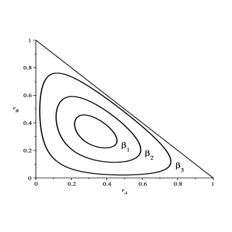
Figure 2: Curves $\Gamma_{\beta}$ in the $r_{A}$-$r_{B}$ plane along which $F(r)$ achieves its minimum value, for $\beta_{1}=3.75$, $\beta_{2}=4.25$, and $\beta_{3}=6.05$ ($\hat{\beta}_{c}=2\pi/\sqrt{3}\simeq 3.63$).

5 Concluding remarks

It is natural to compare the phase diagram obtained here for the one dimensional reflection asymmetric ABC model with that of the corresponding symmetric model, that is, the mean field three state Potts model (see [1],[17]). We will define the latter by replacing the sum over $j>i$ in (1.1) by a sum over all $j\neq i$ and dividing by 2; this yields

$$E_{N}^{*}({\underline{\zeta}})=\frac{1}{2N}[N_{A}N_{C}+N_{C}N_{B}+N_{B}N_{A}]=\frac{1}{4N}[N^{2}-(N_{A}^{2}+N_{B}^{2}+N_{C}^{2})].$$ (5.1)

The energy (5.1) is related to that of the standard mean field Potts model [17] by a choice of energy scale and a shift of the ground state energy. It is, as is usual for mean field models, independent of dimension and geometry. There is thus no spatial structure in the system and the canonical measure just gives equal weights to all configurations.

The canonical free energy functional with prescribed values of $r_{\alpha}=\int_{0}^{1}n_{\alpha}(x)\,dx$ is

$${\cal F}^{*}(\{n\})=\frac{\beta}{2}[r_{A}r_{C}+r_{B}r_{A}+r_{C}r_{B}]-{\mathcal{S}}(\{n\}),$$ (5.2)

with ${\mathcal{S}}\left(\{n\}\right)$ still given by (2.4). For all $\beta$ the minimizers of ${\cal F}^{*}$ are the constant density profiles $\rho_{\alpha}(x)=r_{\alpha}$, and there are no phase transitions of any kind in the canonical system. The corresponding minimum value

$$F^{*}(r)=\frac{\beta}{2}\sum_{\alpha}r_{\alpha}r_{\alpha+2}-\sum_{\alpha}r_{\alpha}\log r_{\alpha}=\frac{\beta}{4}\sum_{\alpha}r_{\alpha}^{2}+\frac{\beta}{4}-\sum_{\alpha}r_{\alpha}\log r_{\alpha}$$ (5.3)

of ${\cal F}^{*}(\{n\})$ is in fact just the value of ${\cal F}(\{n\})$ evaluated at these constant profiles (this follows from our choice of the factor $1/2$ in (5.1)), and hence is an upper bound for the free energy $F(r)$ of (4.16).

The situation is quite different for the grand canonical ensemble. Here the analogue of (4.17) is

$$\hat{F}^{*}(\lambda)=\inf_{r}\,\Bigl{\{}F^{*}(r)-\sum_{\alpha}\lambda_{\alpha}r_{\alpha}\Bigr{\}}$$ (5.4)

The analysis of $F^{*}(\lambda)$ leads to a phase diagram completely different from that of the reflection asymmetric grand canonical model considered in Sections 3 and 4 above [1]. In particular, (5.4) exhibits a first order phase transition for $\lambda_{A}=\lambda_{B}=\lambda_{C}$ at $\beta_{c}^{*}=8\log 2$. For $\beta<\beta_{c}^{*}$ the minimizer is $r_{A}=r_{B}=r_{C}=1/3$; for $\beta>\beta_{c}^{*}$ there are three minimizers, each rich in one of the three species, and at $\beta=\beta_{c}^{*}$ all four of these states are minimizers.

5.1 Higher dimensions

As was already noted and is well known, the standard mean field models with symmetric interactions do not depend on the dimension or topology of the spatial structure of the system considered. This is clearly not the case for models with reflection asymmetric interactions, such as the one-dimensional ABC model considered in this paper.

We comment now on various possible generalizations of such reflection asymmetric mean field models to higher dimensions, taking for simplicity the dimension to be two and the lattice to be an $N\times N$ square in ${\mathbb{Z}}^{2}$. Let us consider first a situation in which the mean field interactions are symmetric in the vertical direction but of the form (1.1) in the horizontal direction. This yields an energy of the form

$$\tilde{E}({\underline{\zeta}}) = {\frac{1}{N^{2}}}\sum_{k,l}^{N}\sum_{i=1}^{N-1}\sum_{j=i+1}^{N}\sum_{\alpha}\eta_{\alpha}(i,k)\eta_{\alpha+2}(j,l)$$ (5.5)

$$= \sum_{i=1}^{N-1}\sum_{j=i+1}^{N}\sum_{\alpha}\tilde{\eta}_{\alpha}(i)\tilde{\eta}_{\alpha+2}(j),$$ (5.6)

where

$$\tilde{\eta}_{\alpha}(i)=\frac{1}{N}\sum_{k=1}^{N}\eta_{\alpha}(i,k).$$ (5.7)

The energy functional $\tilde{\mathcal{E}}$ obtained from (5.6) in the scaling limit is identical to that given in (2.3) with $n_{\alpha}(x)$ replaced by $\tilde{n}_{\alpha}(x)=\int_{0}^{1}n(x,y)\,dy$. The entropy term (compare (2.4)),

$$-\tilde{\mathcal{S}}=\sum_{\alpha}\int_{0}^{1}\int_{0}^{1}n_{\alpha}(x,y)\log n_{\alpha}(x,y)\,dx\,dy,$$ (5.8)

is clearly minimized, subject to a specified $\{\tilde{n}_{\alpha}(x)\}$, by setting $n_{\alpha}(x,y)=\tilde{n}_{\alpha}(x)$, and so density profiles which minimize $\beta\tilde{\mathcal{E}}-\tilde{\mathcal{S}}$ depend only on $x$ and are the same as for the one dimensional case, both for the canonical and grand canonical ensembles.

Remark 5.1.

The two-dimensional chiral clock model [2, 3, 4] also contains interactions—in that case, nearest-neighbor ones—which are reflection symmetric in the vertical direction but not in the horizontal one. When the parameter $\Delta$ (in the notation of [2]) has value $1/2$ the energy, up to an additive constant and a rescaling, is

$$\sum_{i=1}^{N-1}\sum_{k=1}^{N}\sum_{\alpha}\eta_{\alpha}(i,k)\eta_{\alpha+2}(i+1,k)-\sum_{i=1}^{N}\sum_{k=1}^{N-1}\sum_{\alpha}\eta_{\alpha}(i,k)\eta_{\alpha}(i,k+1),$$ (5.9)

so that the interactions in the horizontal direction have a form reminiscent of (1.1).

A second possibility is to take the reflection asymmetry to be the same in the $x$ and $y$ directions. In this case (1.1) takes the form

$$E_{N^{2}}({\underline{\zeta}})={\frac{1}{N^{2}}}\sum_{\alpha}\sum^{N-1}_{i,k=1}\sum^{N}_{\genfrac{}{}{0.0pt}{}{j=i+1}{l=k+1}}\eta_{\alpha}(i,k)\eta_{\alpha+2}(j,l).$$ (5.10)

The analysis of this model seems considerably more complicated and we will attempt no discussion here.

Acknowledgments: We thank Lorenzo Bertini, Thierry Bodineau, Eric Carlen, Or Cohen, Bernard Derrida, and David Mukamel for helpful discussions. The work of J.B. and J.L.L. was supported by NSF Grant DMR-0442066 and AFOSR Grant AF-FA9550-04.

Appendix A Proof of Theorem 4.1(b)

We begin by giving an alternate form of the boundary conditions (4.7). With (2.8) and (2.10) these become

$$\lambda_{\alpha}-\lambda_{\alpha+1}=\log\bigl{(}y_{K}(t_{\alpha}-\beta)\bigr{)}-\log\bigl{(}y_{K}(t_{\alpha}+\beta-\tau_{K}/3)\bigr{)}.$$ (A.1)

From (2.7) and (2.8), $(\log y_{K}(t))^{\prime}=[y_{K}(t+\tau_{K}/3)-y_{K}(t-\tau_{K}/3)]/2$, so that

$$\lambda_{\alpha}-\lambda_{\alpha+1}=\frac{1}{2}\int_{t_{\alpha}+\beta-\tau_{K}/3}^{t_{\alpha}-\beta}\left[y_{K}\left(t+\frac{\tau_{K}}{3}\right)-y_{K}\left(t-\frac{\tau_{K}}{3}\right)\right]\,dt.$$ (A.2)

The solution of (A.2) which also satisfies $\sum_{\alpha}\lambda_{\alpha}=0$ is

$$\lambda_{\alpha}=\frac{1}{2}\int_{s_{\alpha}-(\tau_{K}/6-\beta)}^{s_{\alpha}+(\tau_{K}/6-\beta)}\left(\frac{1}{3}-y_{K}(t)\right)\,dt,$$ (A.3)

where $s_{\alpha}=t_{\alpha}+\tau_{K}/2$. The form (A.3) is convenient when $2\beta\leq\tau_{K}/3$; if $2\beta\geq\tau_{K}/3$ we may rewrite this as

$$\lambda_{\alpha}=\frac{1}{2}\int_{s_{\alpha}-(\beta-\tau_{K}/6)}^{s_{\alpha}+(\beta-\tau_{K}/6)}\left(y_{K}(t)-\frac{1}{3}\right)\,dt.$$ (A.4)

The representations (A.3) and (A.4) are useful because they translate the boundary conditions for the grand canonical model into a form similar to the condition (2.11) in the canonical model.

We need also to recall from [14] some further properties of the function $y_{K}(t)$ and its definite integrals

$$Y(K,s,\delta)=\int_{s-\delta}^{s+\delta}y_{K}(t)\,dt\quad\hbox{and}\quad W(K,s,\delta)=\int_{s-\delta}^{s+\delta}y_{K}\left(t+\frac{\tau_{K}}{3}\right)\,dt.$$ (A.5)

Note that from (2.11),

$$r_{\alpha}=\frac{1}{2\beta}Y(K,t_{\alpha},\beta)$$ (A.6)

and that from (2.10),

$$\lambda_{\alpha} = \frac{\delta}{3}-\frac{1}{2}Y(K,s_{\alpha},\delta)=\frac{\delta}{3}-\frac{1}{2}W(K,s_{\alpha+1},\delta),$$ (A.7)

for $\delta=\tau_{K}/6-\beta\geq 0$, while for $\delta^{\prime}=-\delta>0$,

$$\lambda_{\alpha} = \frac{1}{2}Y(K,s_{\alpha},\delta^{\prime})-\frac{\delta^{\prime}}{3}=\frac{1}{2}W(K,s_{\alpha+1},\delta^{\prime})-\frac{\delta^{\prime}}{3}.$$ (A.8)

Proposition A.1.

For $0<K<1/27$:

(a) (i) $y_{K}(t)$ is even and $\tau_{K}$-periodic (and hence also symmetric about $t=\tau_{K}/2$), takes its minimum value at $t=0$, is strictly increasing on $[0,\tau_{K}/2]$, and takes its maximum value at $t=\tau_{K}/2$. Moreover, (ii) $y_{K}(t-\tau_{K}/3)+y_{K}(t)+y_{K}(t+\tau_{k}/3)=1$ for all $t$.

(b) The minimum value $a=a(K)=y_{K}(0)$ of $y_{K}$ is an increasing function of $K$ satisfying $0<a(K)<1/3$. The maximum value $b=b(K)=y_{K}(\tau_{K}/2)$ is $b=[2-a-\sqrt{4a-3a^{2}}]/2$, and $y_{K}(\tau/6)=(1-b)/2$, $y_{K}(\tau/3)=(1-a)/2$.

(c) (i) For fixed $K$ and $\delta$, with $0<\delta<\tau_{K}/2$, the function $Y(K,t,\delta)$ shares with $y_{K}(t)$ the properties listed in (a.i). Moreover, (ii)

$$Y(K,t-\tau_{K}/3,\delta)+Y(K,t,\delta)+Y(K,t+\tau_{k}/3,\delta)=2\delta.$$ (A.9)

(d) For $0<\delta<\tau_{k}/2$, $Y(K,0,\delta)$ is strictly decreasing, and $W(K,\tau_{k}/6,\delta)$ strictly increasing, in $K$.

Finally, for $0<K_{2}<K_{1}<1/27$:

(e) (i) For any $t_{0}$ the curves $y_{K_{1}}(t_{0}+t)$ and $y_{K_{2}}(t)$ intersect exactly once in the interval $0\leq t\leq\tau_{K_{2}}/2$, and (ii) $y_{K_{2}}(t)<y_{K_{1}}(t)$ and $y_{K_{2}}(\tau_{K_{2}}/2-t)>y_{K_{1}}(\tau_{K_{1}}/2-t)$ for $0\leq t\leq\tau_{K_{1}}/6$.

Proof.

These results either appear in [14] or are immediate consequences of results appearing there. For (a) and (b) see Section 5.2 of [14] and in particular Remark 5.1(a); for (c.i) see Remark 5.3(b). (c.ii) follows from (a.ii). The first statement of (d) follows from the fact that $Y(K,0,\delta)$ is continuous in $K$ and, for $0<\delta<\tau_{k}/2$, approaches $2\delta/3$ as $K\nearrow 1/27$ and $0$ as $K\searrow 0$, together with Theorem 6.1 of [14] which, if one takes there $r_{A}=r_{C}$, asserts that for given $r_{B}$ with $0<r_{B}<1/3$ there is at most one value of $K$ satisfying (A.6). The second statement of (d) is verified similarly. Finally, (e.i) is a special case of Lemma 6.2(a) of [14] and (e.ii) then follows from (e.i) and the inequalities $y_{K_{2}}(0)<y_{K_{1}}(0)$, $y_{K_{2}}(\tau_{K_{1}}/6)<y_{K_{2}}(\tau_{K_{2}}/6)<y_{K_{1}}(\tau_{K_{1}}/6)$, $y_{K_{2}}(\tau_{K_{2}}/2)>y_{K_{1}}(\tau_{K_{1}}/2)$, and $y_{K_{2}}(\tau_{K_{2}}/2-\tau_{K_{1}}/6)>y_{K_{2}}(\tau_{K_{2}}/3)>y_{K_{1}}(\tau_{K_{1}}/3)$, easily obtained from the properties given in (a) and (b). ∎

We now turn to the proof of Theorem 4.1(b). We know (see the remarks at the beginning of Section 4) that there is at least one minimizer and that every minimizer satisfies the ELE (4.6), (4.7). Thus the conclusion of the theorem will follow from:

Lemma A.2.

If $\lambda_{A}$, $\lambda_{B}$, and $\lambda_{C}$ are not all equal then:

(a) No solution of (4.6), (4.7) of type $n$, $n\geq 2$, can minimize $\hat{\cal F}$.

(b) At most one solution of (4.6), (4.7) of type 1 exists.

Remark A.3.

In proving Lemma A.2 we need not consider either the constant solution of the ELE or nonconstant solutions for which $2\beta=(n-2)\beta_{c}/3$, both of which satisfy (4.7) only when all the $\lambda_{\alpha}$ are equal. We may also suppose, without loss of generality, that

$$\lambda_{A}\leq\lambda_{C}\leq\lambda_{B},\quad\hbox{ with $\lambda_{A}<\lambda_{C}$ or $\lambda_{C}<\lambda_{B}$.}$$ (A.10)

If $\delta=\tau_{K}/6-\beta>0$ it then follows from (A.7) that $Y(K,s_{B},\delta)\leq Y(K,s_{C},\delta)\leq Y(K,s_{A},\delta)$ and then from Proposition A.1(c.i) (see Figure 3, which displays graphically the qualitative properties of $Y(K,s,\delta)$ implied there) that $0\leq s_{B}\leq\tau_{K}/6$, so that $\tau_{K}/2\leq t_{B}\leq 2\tau_{K}/3$ and hence, from Proposition A.1(c.i) and (A.6), that $r_{A}\leq r_{C}\leq r_{B}$. If $\lambda_{A}<\lambda_{C}$ then $s_{B}>0$, $t_{B}>\tau_{K}/2$, and $r_{A}<r_{C}$; similarly $r_{C}<r_{B}$, if $\lambda_{C}<\lambda_{B}$. Similarly, if $\tau_{K}/6<\beta<\tau_{K}/2$ then (now using (A.8)) $\tau_{K}/2\leq s_{B}\leq 2\tau_{K}/3$ and $r_{B}\leq r_{C}\leq r_{A}$, again with strict inequality for two of the $\lambda_{\alpha}$ implying the corresponding inequality for the $r_{\alpha}$.

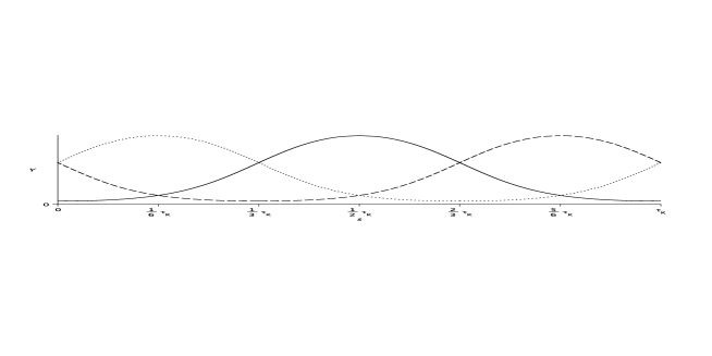
Figure 3: Plots showing qualitative features of $Y(K,s,\delta)$ (solid), $Y(K,s+\tau_{K}/3,\delta)$ (dotted), and $Y(K,s-\tau_{K}/3,\delta)$ (dashed) for $0<\delta<\tau_{K}/2$, based on Proposition A.1(c.1).

Proof of Lemma A.2(a): Consider some type $n$ solution $\rho(x)$, $n\geq 2$, of (4.6), (4.7); $\rho(x)$ has the form (2.8) with $2\beta>\tau_{K}/3$. We need to find a profile $\tilde{\rho}(x)$ with $\hat{\cal F}(\{\tilde{\rho}\})<\hat{\cal F}(\{\rho\})$. There are three subcases:

Case (a.i) $2\beta>\tau_{K}$. In this case it was shown in [14] that there is a rearrangement $\tilde{\rho}(x)$ of $\rho(x)$ with ${\cal F}(\{\tilde{\rho}\})<{\cal F}(\{\rho\})$. This rearrangement does not change the mean densities $r_{\alpha}$ and hence also $\hat{\cal F}(\{\tilde{\rho}\})<\hat{\cal F}(\{\rho\})$.

Case (a.ii) $2\beta=\tau_{K}$. In this case the solution $\rho(x)$ has mean densities $r_{\alpha}=1/3$, so that $\sum\lambda_{\alpha}r_{\alpha}=0$. From the description of the curve $\Gamma$ in Section 4.1 it follows that for some $z>0$ there exists a minimizer $\tilde{\rho}(x)$ of $\hat{\cal F}^{(\beta,0)}$ with mean densities $\tilde{r}_{\alpha}=1/3+z\lambda_{\alpha}$, so that $\sum\lambda_{\alpha}\tilde{r}_{\alpha}>0$. But then

$$\hat{\cal F}^{(\beta,\lambda)}(\{\rho\})=\hat{\cal F}^{(\beta,0)}(\{\rho\})>\hat{\cal F}^{(\beta,0)}(\{\tilde{\rho}\})>\hat{\cal F}^{(\beta,\lambda)}(\{\tilde{\rho}\}).$$ (A.11)

Case (a.iii) $\tau_{K}>2\beta>\tau_{K}/3$. By Remark A.3, $r_{B}\leq r_{C}\leq r_{A}$, with $r_{B}<r_{C}$ if $\lambda_{C}<\lambda_{B}$ and $r_{C}<r_{A}$ if $\lambda_{A}<\lambda_{C}$. Consider now the profile $\tilde{\rho}$ with $\tilde{\rho}_{\alpha}(x)=\rho_{\alpha+1}(x)$. The canonical free energy functional satisfies ${\cal F}(\{\tilde{\rho}\})={\cal F}(\{\rho\})$ and so

$$\hat{\cal F}(\{\tilde{\rho}\})-\hat{\cal F}(\{\rho\}) =\sum_{\alpha}\lambda_{\alpha}r_{\alpha}-\sum_{\alpha}\lambda_{\alpha}r_{\alpha+1}$$ (A.12)

$$\hskip-40.0pt=(\lambda_{A}-\lambda_{C})(r_{A}-r_{B})+(\lambda_{B}-\lambda_{C})(r_{B}-r_{C})<0.$$ (A.13)

∎

The next result, the key to the proof of Lemma A.2(b), gives certain monotonicity properties of $Y(K,s,\delta)$ and $W(K,s,\delta)$.

Lemma A.4.

If $K$, $s$, and $\delta$ satisfy $0<K<1/27$ and $0\leq s,\delta\leq\tau_{K}/6$, then:

(a) For fixed $K$ and $s$ the function $2\delta/3-Y(K,s,\delta)$ (respectively $2\delta/3-W(K,s,\delta)$) is strictly increasing (respectively strictly decreasing) in $\delta$;

(b) For fixed $K$ and $\delta$ the functions $Y(K,s,\delta)$ and $W(K,s,\delta$) are strictly increasing in $s$;

(c) For fixed $s$ and $\delta$ the function $Y(K,s,\delta)$ (respectively $W(K,s,\delta)$) is strictly increasing (respectively strictly decreasing) in $K$.

Proof.

(a) We rely throughout on Proposition A.1(a,b). From $0\leq s+\delta\leq\tau_{K}/3$ and $-\tau_{K}/6\leq s-\delta\leq\tau_{K}/6$ it follows that $y_{K}(s+\delta)\leq(1-a)/2$ and $y_{K}(s-\delta)\leq(1-b)/2$. Then from (A.5),

$$\frac{d}{d\delta}\left[\frac{2\delta}{3}-Y(K,s,\delta)\right]=\frac{2}{3}-y_{K}(s+\delta)-y_{K}(s-\delta)\geq\frac{a+b}{2}-\frac{1}{3}>0,$$ (A.14)

as is easily verified from $b=[2-a-\sqrt{4a-3a^{2}}]/2$ with $0<a<1/3$. To show that $(d/d\delta)(2\delta/3-W(K,s,\delta))<0$ it suffices similarly to verify that

$$z(K,s,\delta):=y_{K}\left(s+\frac{\tau_{K}}{3}+\delta\right)+y_{K}\left(s+\frac{\tau_{K}}{3}-\delta\right)>\frac{2}{3}.$$ (A.15)

Because $y_{K}$ is even and $\tau_{K}$-periodic, $z$ is invariant under $(s,\delta)\to(s^{\prime},\delta^{\prime})$ with $s^{\prime}=\tau_{K}/6-\delta$, $\delta^{\prime}=\tau_{K}/6-s$, so that it suffices to verify (A.15) for $s+\delta\leq\tau_{K}/6$, and since under this condition both terms in $z(K,s,\delta)$ are increasing in $s$ it suffices to consider $s=0$. But because $y_{K}$ is even,

$$z(K,0,\delta) = \frac{1}{2}\Bigl{[}y_{K}\left(\frac{\tau_{K}}{3}+\delta\right)+y_{K}\left(-\frac{\tau_{K}}{3}+\delta\right)$$ (A.16)

$$\hskip 40.0pt+y_{K}\left(-\frac{\tau_{K}}{3}-\delta\right)+y_{K}\left(\frac{\tau_{K}}{3}-\delta\right)\Bigr{]}$$

$$= 1-\frac{1}{2}\left[y_{K}(\delta)+y_{K}(-\delta)\right]\geq\frac{1+b}{2}>2/3.$$

(b) See Proposition A.1(c).

(c) The proofs for $Y$ and of $W$ are similar and we check only $Y$. Suppose that $0<K_{2}<K_{1}<1/27$ and that for some $s_{*}\in[0,\tau_{K_{1}}/6]$,

$$Y(K_{1},s_{*},\delta)\leq Y(K_{2},s_{*},\delta).$$ (A.17)

Then certainly $y_{K_{1}}(t_{*})<y_{K_{2}}(t_{*})$ for some $t_{*}\in[s_{*}-\delta,s_{*}+\delta]$, and since $y_{K_{1}}(0)>y_{K_{2}}(0)$, Proposition A.1(e.i) implies that $y_{K_{1}}(t)\leq y_{K_{2}}(t)$ for $t\in[t_{*},\tau_{K_{1}}/3]$. Then for $s\in[s_{*},\tau_{K_{1}}/6]$,

$$\frac{d}{ds}\left[Y(K_{2},s,\delta)-Y(K_{1},s,\delta)\right]\hskip-130.0pt$$ (A.18)

$$= \left[y_{K_{1}}(s-\delta)-y_{K_{2}}(s-\delta)\right]+\left[y_{K_{2}}(s+\delta)-y_{K_{1}}(s+\delta)\right]$$

$$> 0,$$

since both terms on the right had side are positive. But for $0\leq\delta\leq\tau_{K_{1}}/6$,

$$W(K_{1},\tau_{K_{1}}/6,\delta)<W(K_{2},\tau_{K_{2}}/6,\delta),$$ (A.19)

by Proposition A.1(e.ii), and so from Proposition A.1(a),

$$Y(K_{1},\tau_{K_{1}}/6,\delta) = \frac{1}{2}\int_{\tau_{K_{1}}/6-\delta}^{\tau_{K_{1}}/6+\delta}\left[y_{K_{1}}\left(t-\frac{\tau_{K_{1}}}{3}\right)+y_{K_{1}}(t)\right]\,dt$$ (A.20)

$$= \frac{1}{2}\int_{\tau_{K_{1}}/6-\delta}^{\tau_{K_{1}}/6+\delta}\left[1-y_{K_{1}}\left(t+\frac{\tau_{K_{1}}}{3}\right)\right]\,dt$$

$$= \delta-\frac{1}{2}W(K_{1},\tau_{K_{1}}/6,\delta)$$

$$> \delta-\frac{1}{2}W(K_{2},\tau_{K_{2}}/6,\delta)$$

$$= Y(K_{2},\tau_{K_{2}}/6,\delta)$$

$$> Y(K_{2},\tau_{K_{1}}/6,\delta)$$

since $\tau_{K_{1}}<\tau_{K_{2}}$ (see Remark 2.1), contradicting (A.17) and (A.18). ∎

Proof of Lemma A.2(b): For type 1 solutions we have from (A.7) that

$$\lambda_{B}=\frac{\delta}{3}-\frac{1}{2}Y(K,s_{B},\delta),\qquad\lambda_{A}=\frac{\delta}{3}-\frac{1}{2}W(K,s_{B},\delta),$$ (A.21)

with $\delta=\tau_{K}/6-\beta>0$ and, by Remark A.3, $0\leq s_{B}\leq\tau_{K}/6$. Thus the existence for some $\lambda$ of two type 1 solutions would correspond to the existence of $(K_{1},s_{1})$ and $(K_{2},s_{2})$ with $0<K_{2}<K_{1}<1/27$ and $0\leq s_{i}\leq\tau_{K_{i}}/6$, $i=1,2$, such that $2\delta_{1}/3-Y(K_{1},s_{1},\delta_{1})=2\delta_{2}/3-Y(K_{2},s_{2},\delta_{2})$ and $2\delta_{1}/3-W(K_{1},s_{1},\delta_{1})=2\delta_{2}/3-W(K_{2},s_{2},\delta_{2})$, where $\delta_{i}=\tau_{K_{i}}/6-\beta$ for $i=1,2$. Then from Lemma A.4(a,c),

$$\frac{2\delta_{2}}{3}-Y(K_{2},s_{2},\delta_{2}) = \frac{2\delta_{1}}{3}-Y(K_{1},s_{1},\delta_{1})$$ (A.22)

$$< \frac{2\delta_{1}}{3}-Y(K_{2},s_{1},\delta_{1})$$

$$< \frac{2\delta_{2}}{3}-Y(K_{2},s_{1},\delta_{2}),$$

so that Lemma A.4(b) implies that $s_{1}<s_{2}$. But also

$$\frac{2\delta_{2}}{3}-W(K_{2},s_{2},\delta_{2}) = \frac{2\delta_{1}}{3}-W(K_{1},s_{1},\delta_{1})$$ (A.23)

$$> \frac{2\delta_{1}}{3}-W(K_{2},s_{1},\delta_{1})$$

$$> \frac{2\delta_{2}}{3}-W(K_{2},s_{1},\delta_{2}),$$

implying that $s_{1}>s_{2}$, a contradiction. ∎