Counterintuitive transitions between crossing energy levels

Abstract

We calculate analytically the probabilities for intuitive and counterintuitive transitions in a three-state system, in which two parallel energies are crossed by a third, tilted energy. The state with the tilted energy is coupled to the other two states in a chainwise linkage pattern with constant couplings of finite duration. The probability for a counterintuitive transition is found to increase with the square of the coupling and decrease with the squares of the interaction duration, the energy splitting between the parallel energies and the tilt (chirp) rate. Physical examples of this model can be found in coherent atomic excitation and optical shielding in cold atomic collisions.

I Introduction

The famous Landau-Zener (LZ) model LZ is the most popular tool for estimating the transition probability between two states whose energies cross in time. This model assumes a constant interaction of infinite duration and linear energies. Owing to some mathematical subtleties, the LZ model often provides more accurate results than anticipated (given the rather simple time dependence of the LZ Hamiltonian) when applied to real physical systems with more sophisticated time dependences. The popularity of the LZ model is further motivated by the extreme simplicity of the transition probability.

The LZ model has been extended to three and more levels by a number of authors. There are two main types of generalizations: single-crossing (bow-tie) models and multiple-crossings grid models.

In the bow-tie models all state energies cross at the same instant of time. Carroll and Hioe have solved the three-state bow-tie model in a special symmetric case Carroll-special and in the general case Carroll-general . An extension of this model to $N$ states has been suggested Harmin ; Brundobler and then rigorously derived by Ostrovsky and Nakamura Ostrovsky97 . A further extension, wherein one of the levels is split into two parallel levels, has been suggested Demkov00 and derived Demkov01 by Demkov and Ostrovsky. An example of a bow-tie system occurs when a sequentially coupled quantum ladder of states in an atom or a molecule is driven by chirped laser pulses ARPC ; an adiabatic sweep of frequency through resonance will transfer all population from the lowest to the highest energy state, for either sign of the chirp. A bow-tie type of linkage can also occur in a rf-pulse controlled Bose-Einstein condensate output coupler Mewes ; VitanovBEC . Yet another example is the coupling pattern of Rydberg sublevels in a magnetic field Harmin .

In the multiple-crossings grid models the energy diagram consists of a grid of crossings formed by two manifolds of rectilinear parallel diabatic energies that cross each other. In the Demkov-Osherov (DO) model Demkov68 ; Kayanuma , a single tilted energy crosses a set of $N$ parallel energies. This model has been generalized to the case when the single tilted energy is replaced by a set of $M$ parallel energies, which cross the other set of $N$ parallel energies Demkov95 ; Usuki ; Ostrovsky98 . The special case when $M$ and $N$ are infinite (so that the grid of crossings is periodic) has also been solved Demkov95b . Effects of level degeneracies and quasi-degeneracies have been studied by Yurovsky and Ben-Reuven Yurovsky98 ; Yurovsky01 .

In the most general case of an asymmetric linear Hamiltonian, $\mathsf{H}(t)=\mathsf{A}+\mathsf{B}t$, where $\mathsf{B}$ is diagonal, the general solution has not been derived yet, but exact results for some “survival” probabilities have been conjectured Brundobler and derived Shytov ; Sinitsyn04 ; Volkov04 ; Volkov05 .

A variety of physical systems provide examples of multiple level crossings. Amongst them we mention ladder climbing of atomic and molecular states by chirped laser pulses climbing , optical shielding in cold atomic collisions Suominen96a ; Suominen96b ; Yurovsky97 ; Napolitano ; Piilo , optical centrifuge for molecules centrifuge , Stark-chirped rapid adiabatic passage (SCRAP) SCRAP-theory ; SCRAP-experiment ; SCRAP-3S , and creation of entaglement in many-particle systems entanglement . In fact, physical situations where multiple level crossings play a role have been discussed already in 1960’s, when the harpoon model for reactive scattering was considered Child . If one adds the vibrational states to the scattering picture, then one obtains a multilevel crossing model, which has been studied using the LZ model Child .

A general feature of all soluble multilevel models is that the transition probabilities $P_{m\rightarrow n}$ between states $\psi_{m}$ and $\psi_{n}$ are given by very simple expressions, as in the original LZ model, although the derivations are usually quite involved. In the grid models in particular, such as the DO model, the exact probabilities $P_{m\rightarrow n}$ have the same form — products of LZ probabilities for transition or no-transition applied at the relevant crossings — as what would be obtained by naive multiplication of LZ probabilities while moving across the grid of crossings from $\psi_{m}$ to $\psi_{n}$, without accounting for phases and interferences.

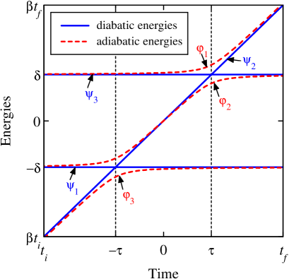
Figure 1: (Color online) Diabatic and adiabatic energies in the three-state crossing model studied in this paper. We are concerned primarily with the (counterintuitive) transition $\psi_{3}\rightarrow\psi_{1}$.

A very interesting feature of all grid models is that counterintuitive transitions, for which the level crossings appear in a “wrong” order, are forbidden. In the three-state example in Fig. 1 such is the transition $\psi_{3}\rightarrow\psi_{1}$. In the adiabatic limit, the inhibition of such transitions is easily understood: for the $\psi_{3}\rightarrow\psi_{1}$ transition an adiabatic path requires the level crossing between $\psi_{3}$ and $\psi_{2}$ to occur before the crossing between $\psi_{2}$ and $\psi_{1}$; this is not the case here and hence there is no adiabatic path linking $\psi_{3}$ to $\psi_{1}$. In the general case of nonadiabatic evolution, however, the inhibition of the $\psi_{3}\rightarrow\psi_{1}$ transition is not so obvious because the concerned final state $\psi_{1}$ acquires some nonzero transient population during the interaction. Yet in the end this population vanishes, and this is an exact result. A similar conclusion applies to more general level-crossing models Sinitsyn04 ; Volkov05 as well.

We have verified with numerical simulations that all ingredients of the multilevel LZ models are essential for this feature: linear energies, constant interactions and infinite duration. Nonlinear energies, pulsed interactions or finite interaction duration can each lead to nonzero probability for counterintuitive transitions.

Yurovsky et al. Yurovsky99 have studied analytically and numerically the counterintuitive transition probability in two variations of the DO model: (i) with a finite interaction duration and (ii) with a piecewise-linear sloped potential. They have used a perturbative approach assuming a quasidegenerate band of parallel energies and have found nonzero probabilities for counterintuitive transitions in both models.

In this paper, we derive analytically the probability for a counterintuitive transition in the simplest case of the DO model involving three states, with two parallel and one slanted energy, as shown in Fig. 1. We assume a finite interaction duration, but our approach does not use the quasidegeneracy assumption of Yurovsky et al. Yurovsky99 ; therefore our results are more general, as far as the three-state case is concerned. The purpose of this work is not just to show that the probability for a counterintuitive transition is nonzero but rather to derive accurate analytical estimates for it. Our approach involves transformation to the adiabatic basis where the evolution is represented as a sequence of instantaneous two-state LZ transitions at each crossing and adiabatic evolution elsewhere. This approach allows us to derive the transition probabilities between each pair of diabatic states, including the probability for the counterintuitive transition.

The problem of counterintuitive transitions, besides quite interesting by itself, has interesting physical implications, which are discussed in some detail in Sec. VI. Amongst them, we mention the problem of saturated optical schielding with near-resonant light, which plays an important role in cold atomic collisions Suominen96a ; Suominen96b ; Yurovsky97 ; Napolitano ; Piilo .

This paper is organized as follows. We define the problem in Sec. II and the propagator is derived in Sec. III in the general case. The transition probabilities in the finite DO model are derived and compared with numerical results in Sec. IV. The time-dependent probabilities in the original (infinite) DO model are presented in Sec. V. Some physical examples of counterintuitive transitions are discussed in Sec. VI. The conclusions are summarized in Sec. VII.

II Definition of the problem

II.1 The system

The probability amplitudes of the three-state system $\mathbf{C}(t)=[C_{1}(t),C_{2}(t),C_{3}(t)]^{T}$ with the energies shown in Fig. 1 satisfy the Schrödinger equation ($\hbar=1$),

$$i\mathbf{\dot{C}}(t)=\mathsf{H}(t)\mathbf{C}(t),$$ (1)

where the overdot denotes $d/dt$. The Hamiltonian in the usual rotating-wave approximation is given by Shore

$$\mathsf{H}(t)=\left[\begin{array}[]{ccc}-\delta&\Omega_{12}&0\\ \Omega_{12}&\beta t&\Omega_{23}\\ 0&\Omega_{23}&\delta\end{array}\right].$$ (2)

As the Hamiltonian (2) shows, there is no direct coupling between states $\psi_{1}$ and $\psi_{3}$ but each of them is coupled to state $\psi_{2}$. Without loss of generality the constant couplings $\Omega_{12}$ and $\Omega_{23}$ will be assumed real and positive. Both couplings are supposed to have the same finite duration, being turned on at time $t_{i}$ and turned off at time $t_{f}$. In the original DO model the couplings last from $-\infty$ to $+\infty$. Furthermore, the energy splitting parameter $\delta$ and the slope $\beta$ of the energy of state $\psi_{2}$ are assumed positive too,

$$\delta>0,\qquad\beta>0.$$ (3)

Given these assumptions, the crossing between the diabatic energies of states $\psi_{1}$ and $\psi_{2}$, occuring at time $t_{-}=-\tau$ precedes the crossing between states $\psi_{2}$ and $\psi_{3}$, occuring at time $t_{+}=\tau$, where

$$\tau=\frac{\delta}{\beta}.$$ (4)

Therefore, the transition $\psi_{1}\rightarrow\psi_{3}$ is intuitive, while the opposite transition $\psi_{3}\rightarrow\psi_{1}$ is counterintuitive. In the adiabatic limit, the transition probability from $\psi_{1}$ to $\psi_{3}$ is $P_{1\rightarrow 3}=1$, whereas that from $\psi_{3}$ to $\psi_{1}$ is $P_{3\rightarrow 1}=0$.

II.2 The Demkov-Osherov model

In the DO model the transition probabilities $P_{m\rightarrow n}$ from state $\psi_{m}$ at $t\rightarrow-\infty$ to state $\psi_{n}$ at $t\rightarrow+\infty$ are given exactly by products of two-state single-crossing LZ probabilities, as follows

$$\begin{array}[]{lll}P_{1\rightarrow 1}=p_{-},&P_{1\rightarrow 2}=q_{-}p_{+},&P_{1\rightarrow 3}=q_{-}q_{+},\\ P_{2\rightarrow 1}=q_{-},&P_{2\rightarrow 2}=p_{-}p_{+},&P_{2\rightarrow 3}=p_{-}q_{+},\\ P_{3\rightarrow 1}=0,&P_{3\rightarrow 2}=q_{+},&P_{3\rightarrow 3}=p_{+},\end{array}$$ (5)

where

$$p_{\pm}=e^{-2\pi\alpha_{\pm}^{2}},\qquad q_{\pm}=1-p_{\pm},$$ (6)

i.e. $q_{\pm}$ is the transition probability and $p_{\pm}$ is the probability of no transition at the crossing $t_{\pm}$, with

$$\alpha_{-}=\Omega_{12}/\beta^{\frac{1}{2}},\qquad\alpha_{+}=\Omega_{23}/\beta^{\frac{1}{2}}.$$ (7)

These simple results coincide with what would be expected naively, by treating the crossings independently, no matter how close they are to each other, and multiplying LZ probabilities. In particular, if the system is initially in state $\psi_{3}$, the transition probability to state $\psi_{1}$ is exactly zero at $t\rightarrow+\infty$, $P_{3\rightarrow 1}=0$, which means that the counterintuitive transition $\psi_{3}\rightarrow\psi_{1}$ is forbidden. This zero probability is rather unexpected because state $\psi_{1}$ acquires some nonzero population during the interaction. However, it vanishes at $t\rightarrow+\infty$ for any set of parameters, irrespective of whether the interaction is adiabatic or not. This property is unique for the DO model and it depends crucially on any of its features: infinite coupling durations, constant couplings, constant energies of states $\psi_{1}$ and $\psi_{3}$ and linear energy of state $\psi_{2}$. The goal of the present paper is to estimate the probability for counterintuive transitions in the case of finite coupling duration.

III Transition matrix

III.1 Eigenvalues and eigenstates

We need the eigenvalues and the eigenstates (the adiabatic states) of $\mathsf{H}(t)$. The eigenvalues read Shore

$$\lambda_{1} = -\frac{1}{3}a+\frac{2}{3}s\cos\frac{1}{3}\theta,$$ (8a)

$$\lambda_{2} = -\frac{1}{3}a-\frac{2}{3}s\cos\frac{1}{3}(\theta+\pi),$$ (8b)

$$\lambda_{3} = -\frac{1}{3}a-\frac{2}{3}s\cos\frac{1}{3}(\theta-\pi),$$ (8c)

where

$$a = -\beta t,$$ (9a)

$$b = -(\delta^{2}+\Omega_{12}^{2}+\Omega_{23}^{2}),$$ (9b)

$$c = \delta(\Omega_{12}^{2}-\Omega_{23}^{2}+\delta\beta t),$$ (9c)

$$s = \sqrt{a^{2}-3b},$$ (9d)

$$\cos\theta = -\frac{2a^{3}-9ab+27c}{2s^{3}}.$$ (9e)

The eigenstates are given by $$\varphi_{k}=[f_{1k},f_{2k},f_{3k}]^{T}$$, with

$$f_{1k} = \frac{1}{N_{k}}\Omega_{12}(\lambda_{k}-\delta),$$ (10a)

$$f_{2k} = \frac{1}{N_{k}}(\lambda_{k}^{2}-\delta^{2}),$$ (10b)

$$f_{3k} = \frac{1}{N_{k}}\Omega_{23}(\lambda_{k}+\delta),$$ (10c)

where $$N_{k} k=1,2,3$$ are normalization factors (). The asymptotic behaviors at large times of the eigenvalues and the eigenstates are presented in Appendix A.

III.2 Adiabatic basis

The transformation linking the diabatic amplitudes $\mathbf{C}(t)$ and the adiabatic amplitudes $\mathbf{A}(t)$ is given by

$$\mathbf{C}(t)=\mathsf{F}(t)\mathbf{A}(t),$$ (11)

where $\mathbf{A}(t)=[A_{1}(t),A_{2}(t),A_{3}(t)]^{T}$ and $\mathsf{F}(t)$ is an orthogonal rotation matrix [$\mathsf{F}^{-1}(t)=\mathsf{F}^{T}(t)$] whose columns are the eigenvectors (10),

$$\mathsf{F}(t)=\left[\begin{array}[]{ccc}f_{11}(t)&f_{12}(t)&f_{13}(t)\\ f_{21}(t)&f_{22}(t)&f_{23}(t)\\ f_{31}(t)&f_{32}(t)&f_{33}(t)\end{array}\right].$$ (12)

The Schrödinger equation in the adiabatic basis reads

$$i\mathbf{\dot{A}}(t)=\mathsf{H}_{A}(t)\mathbf{A}(t),$$ (13)

with $\mathsf{H}_{A}(t)=\mathsf{F}^{T}(t)\mathsf{H}(t)\mathsf{F}(t)-i\mathsf{F}^{T}(t)\dot{\mathsf{F}}(t)$, or

$$\mathsf{H}_{A}(t)=\left[\begin{array}[]{ccc}\lambda_{1}&-i\nu_{12}&-i\nu_{13}\\ -i\nu_{21}&\lambda_{2}&-i\nu_{23}\\ -i\nu_{31}&-i\nu_{32}&\lambda_{3}\end{array}\right],$$ (14)

where the nonadiabatic coupling between the adiabatic states $\varphi_{k}(t)$ and $\varphi_{l}(t)$ is

$$\nu_{kl}(t)=\langle\varphi_{k}(t)\mid\dot{\varphi}_{l}(t)\rangle=-\nu_{lk}(t)$$ (15)

We use the fact that the transition times in the adiabatic basis are shorter than in the diabatic basis LZtimes . This is so because while the asymptotic behaviors of the adiabatic energies at large times (42) are approximately the same as the asymptotics of the diabatic energies, the couplings $\nu_{kl}$ in the adiabatic basis (15) vanish as $t^{-2}$ [see Eqs. (42)], in contrast to the constant couplings $\Omega_{12}$ and $\Omega_{23}$ in the diabatic basis. The difference in the transition times is illustrated in Fig. 2, where the oscillations in the populations of the adiabatic states vanish much faster.

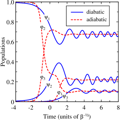
Figure 2: (Color online) Time evolutions of the populations of the diabatic and adiabatic states for the original DO model ($t_{i}=-\infty$). The system starts in state $\psi_{1}$. The interaction parameters are $\Omega_{12}=\Omega_{23}=\beta^{\frac{1}{2}}$, $\delta=\beta^{\frac{1}{2}}$.

III.3 Evolution matrix in the adiabatic basis

Our method is based on two simplifying assumptions. First, we assume that appreciable transitions take place only between neighboring adiabatic states, $\varphi_{1}(t)\leftrightarrow\varphi_{2}(t)$ and $\varphi_{2}(t)\leftrightarrow\varphi_{3}(t)$, but not between states $\varphi_{1}(t)$ and $\varphi_{3}(t)$, because the energies of the latter pair are split by the largest gap. Second, we assume that the nonadiabatic transitions occur instantly at the corresponding avoided crossings and the evolution is adiabatic elsewhere. This allows us to obtain the propagator in the adiabatic basis by multiplying five simple transition matrices describing LZ transitions or adiabatic evolution.

The adiabatic evolution matrix $\mathsf{U}^{A}(t_{f},t_{i})$ is most conveniently determined in the adiabatic interaction representation, where the diagonal elements of $\mathsf{H}_{A}(t)$ are nullified. The transformation reads

$$\mathbf{A}(t)=\mathsf{M}(t)\mathbf{B}(t),$$ (16)

where

$$\mathsf{M}(t,t_{0})=\left[\begin{array}[]{ccc}e^{-i\Lambda_{1}(t,t_{0})}&0&0\\ 0&e^{-i\Lambda_{2}(t,t_{0})}&0\\ 0&0&e^{-i\Lambda_{3}(t,t_{0})}\end{array}\right],$$ (17)

$$\Lambda_{k}(t,t_{0}) = \int_{t_{0}}^{t}\lambda_{k}(t^{\prime})dt^{\prime},$$ (18a)

$$\Lambda_{kl}(t,t_{0}) \equiv \Lambda_{k}(t,t_{0})-\Lambda_{l}(t,t_{0}),$$ (18b)

and $$t_{0}$$ is an arbitrary fixed time. The Schrödinger equation in this basis reads

$$i\mathbf{\dot{B}}(t)=\mathsf{H}_{B}(t)\mathbf{B}(t),$$ (19)

with

$$\mathsf{H}_{B}(t)=-i\left[\begin{array}[]{ccc}0&\nu_{12}e^{i\Lambda_{12}(t,t_{0})}&\nu_{13}e^{i\Lambda_{13}(t,t_{0})}\\ \nu_{21}e^{i\Lambda_{21}(t,t_{0})}&0&\nu_{23}e^{i\Lambda_{23}(t,t_{0})}\\ \nu_{31}e^{i\Lambda_{31}(t,t_{0})}&\nu_{32}e^{i\Lambda_{32}(t,t_{0})}&0\end{array}\right].$$ (20)

In this basis, the evolution matrix for adiabatic evolution is given by the identity matrix.

The LZ transitions at the crossings at $\pm\tau$ are described by the transition matrices

$$\mathsf{U}_{LZ}(-\tau) = \left[\begin{array}[]{ccc}1&0&0\\ 0&\sqrt{q_{-}}e^{-i\phi_{-}}&-\sqrt{p_{-}}\\ 0&\sqrt{p_{-}}&\sqrt{q_{-}}e^{i\phi_{-}}\end{array}\right],$$ (21d)

$$\mathsf{U}_{LZ}(\tau) = \left[\begin{array}[]{ccc}\sqrt{q_{+}}e^{-i\phi_{+}}&-\sqrt{p_{+}}&0\\ \sqrt{p_{+}}&\sqrt{q_{+}}e^{i\phi_{+}}&0\\ 0&0&1\end{array}\right],$$ (21h)

where $p_{\pm}$ and $q_{\pm}$ are given by Eqs. (6) and

$$\phi_{\pm}=\arg\Gamma(1-i\alpha_{\pm}^{2})+\frac{\pi}{4}+\alpha_{\pm}^{2}\left(\ln\alpha_{\pm}^{2}-1\right),$$ (22)

with $\alpha_{\pm}$ given by Eqs. (7). The LZ phases $\phi_{\pm}$ do not depend on time, unlike the dynamical phases (18a).

The propagator in the adiabatic basis reads $\mathsf{U}^{A}(t_{f},t_{i})=\mathsf{M}(t_{f},\tau)\mathsf{U}_{LZ}(\tau)\mathsf{M}(\tau,-\tau)\mathsf{U}_{LZ}(-\tau)\mathsf{M}(-\tau,t_{i})$, or

$${\sf U}^{A}(t_{f},t_{i})=\left[\begin{array}[]{ccc}\sqrt{q_{+}}e^{-i\phi_{+}-i\Lambda_{1}(t_{f},t_{i})}&-\sqrt{p_{+}q_{-}}e^{-i\phi_{-}-i\Lambda_{1}(t_{f},\tau)-i\Lambda_{2}(\tau,t_{i})}&\sqrt{p_{-}p_{+}}e^{-i\Lambda_{1}(t_{f},\tau)-i\Lambda_{2}(\tau,-\tau)-i\Lambda_{3}(-\tau,t_{i})}\\ \sqrt{p_{+}}e^{-i\Lambda_{1}(\tau,t_{i})-i\Lambda_{2}(t_{f},\tau)}&\sqrt{q_{-}q_{+}}e^{i(\phi_{+}-\phi_{-})-i\Lambda_{2}(t_{f},t_{i})}&-\sqrt{p_{-}q_{+}}e^{i\phi_{+}-i\Lambda_{2}(t_{f},-\tau)-i\Lambda_{3}(-\tau,t_{i})}\\ 0&\sqrt{p_{-}}e^{-i\Lambda_{2}(-\tau,t_{i})-i\Lambda_{3}(t_{f},-\tau)}&\sqrt{q_{-}}e^{i\phi_{-}-i\Lambda_{3}(t_{f},t_{i})}\end{array}\right],$$ (23)

In the special case when $t_{i}=-T$, $t_{f}=T$ and $\Omega_{12}=\Omega_{23}\equiv\Omega$, many expressions simplify, as shown in Appendix B. Then $\alpha_{+}=\alpha_{-}\equiv\alpha$, $p_{+}=p_{-}\equiv p$, $q_{+}=q_{-}\equiv q=1-p$, and Eq. (23) reduces to

$${\sf U}^{A}(T,-T)=\left[\begin{array}[]{ccc}\sqrt{q}\ e^{-i\phi-i\Lambda_{1}(T,-T)}&-\sqrt{pq}\ e^{-i\phi-i\Lambda_{12}(T,\tau)}&p\\ \sqrt{p}\ e^{i\Lambda_{3}(T,-\tau)-i\Lambda_{2}(T,\tau)}&q&-\sqrt{pq}\ e^{i\phi+i\Lambda_{12}(T,\tau)}\\ 0&\sqrt{p}\ e^{i\Lambda_{2}(T,\tau)-i\Lambda_{3}(T,-\tau)}&\sqrt{q}\ e^{i\phi+i\Lambda_{1}(T,-T)}\end{array}\right].$$ (24)

III.4 Evolution matrix in the diabatic basis

The propagator in the diabatic basis can be obtained by using the transformation (11); it reads

$$\mathsf{U}(t_{f},t_{i})=\mathsf{F}(t_{f})\mathsf{U}^{A}(t_{f},t_{i})\mathsf{F}^{T}(t_{i}).$$ (25)

We shall use this relation to derive the transition probabilities in the finite and original DO models below.

IV Transition Probabilities in the finite Demkov-Osherov model

IV.1 The propagator

In order to obtain simpler formulas for the probabilities we assume that $t_{i}=-T$, $t_{f}=T$, although our approach is not limited to these restrictions. The transition probability from state $\psi_{m}$ to $\psi_{n}$ is given by $P_{m\rightarrow n}=\left|U_{nm}(T,-T)\right|^{2}$, where

$$U_{nm}(T,-T)=\sum_{k,l=1}^{3}f_{nk}(T)U_{kl}^{A}(T,-T)f_{ml}(-T).$$ (26)

Using this relation one can calculate the transition probability between any two states of the system. We pay special attention to the probability for counterintuitive transitions $P_{3\rightarrow 1}$, which is zero in the original DO model.

IV.2 Counterintuitive transition

In the special case of equal couplings, $\Omega_{12}=\Omega_{23}\equiv\Omega$, we find from Eqs. (24), (26) and (46) that the transition probability $P_{3\rightarrow 1}=|U_{13}(T,-T)|^{2}$ reads

$$P_{3\rightarrow 1} = \big{|}pf_{11}^{2}+qf_{12}^{2}-2\sqrt{pq}f_{11}f_{12}\cos[\Lambda_{12}(T,\tau)+\phi]$$ (27)

$$+2\sqrt{p}f_{12}f_{13}\cos[\Lambda_{2}(T,\tau)-\Lambda_{3}(T,-\tau)]$$

$$+2\sqrt{q}f_{11}f_{13}\cos[\Lambda_{1}(T,-T)+\phi]\big{|}^{2}.$$

It can be written as

$$P_{3\rightarrow 1}=\overline{P_{3\rightarrow 1}}+\widetilde{P_{3\rightarrow 1}},$$ (28)

where $\overline{P_{3\rightarrow 1}}$ is the average probability and $\widetilde{P_{3\rightarrow 1}}$ is the oscillating part. By using the asymptotic expansions (43) for $f_{mn}$ in Appendix A and keeping the leading terms in the expansion over $1/T$ we find

$$\overline{P_{3\rightarrow 1}} = (pf_{11}^{2}+qf_{12}^{2})^{2}+2(qf_{11}^{2}+pf_{12}^{2})f_{13}^{2}+2pqf_{11}^{2}f_{12}^{2}$$ (29a)

$$\sim \frac{\Omega^{2}(\Omega^{2}p+4\delta^{2}q)}{2\delta^{2}\beta^{2}T^{2}}+\frac{\Omega^{2}(\Omega^{4}p-8\delta^{4}q)}{2\delta^{3}\beta^{3}T^{3}}+\dots,$$ (29b)

$$\widetilde{P_{3\rightarrow 1}} \sim \frac{\Omega^{2}}{\beta^{2}T^{2}}\left\{4q\cos^{2}[\Lambda_{1}(T,-T)+\phi]\right.$$ (30)

$$+\frac{p\Omega^{2}}{\delta^{2}}\cos^{2}\left[\Lambda_{2}(T,\tau)-\Lambda_{3}(T,-\tau)\right]$$

$$-\frac{4\sqrt{pq}\Omega}{\delta}\cos[\Lambda_{1}(T,-T)+\phi]$$

$$\times\left.\cos\left[\Lambda_{2}(T,\tau)-\Lambda_{3}(T,-\tau)\right]\right\}+\dots$$

For unequal couplings ($\Omega_{12}\neq\Omega_{23}$), the expansion over $1/T$ of the average probability reads

$$\overline{P_{3\rightarrow 1}} \sim \frac{\Omega_{12}^{2}\Omega_{23}^{2}(p_{-}+p_{+})+4\delta^{2}(\Omega_{12}^{2}q_{+}+\Omega_{23}^{2}q_{-})}{4\delta^{2}\beta^{2}T^{2}}$$ (31)

$$+ \frac{\Omega_{12}^{2}\Omega_{23}^{2}(\Omega_{12}^{2}p_{-}+\Omega_{23}^{2}p_{+})-8\delta^{4}(\Omega_{12}^{2}q_{+}+\Omega_{23}^{2}q_{-})}{4\delta^{3}\beta^{3}T^{3}}$$

$$+ \dots$$

The part $\widetilde{P_{3\rightarrow 1}}$ is too cumbersome to be presented here.

In the near-adiabatic regime ($\alpha\gg 1$, $p\ll 1$, $q\approx 1$, and $\phi\ll 1$), we find from Eq. (27) that

$$P_{3\rightarrow 1}\sim\frac{4\Omega^{2}}{\beta^{2}T^{2}}\cos^{2}[\Lambda_{1}(T,-T)+\phi].$$ (32)

In the weak-coupling limit ($\alpha\ll 1$, $p\approx 1$, $q\ll 1$, and $\phi\approx\pi/4$), we find from Eq. (27) that

$$P_{3\rightarrow 1}\sim\frac{\Omega^{4}}{\delta^{2}\beta^{2}T^{2}}\cos^{2}[\Lambda_{2}(T,\tau)-\Lambda_{3}(T,-\tau)].$$ (33)

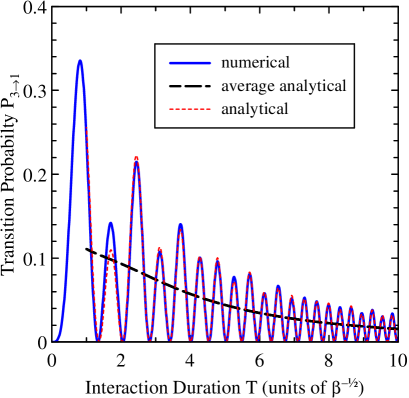
Figure 3: (Color online) Probability for counterintuitive transition $P_{3\rightarrow 1}$ plotted against the coupling duration $T$ for interaction parameters $\Omega_{12}=\Omega_{23}=\beta^{\frac{1}{2}}$, $\delta=\beta^{\frac{1}{2}}$. The full line shows numerical results, the thin dashed curve the analytical approximation (27) and the thick dashed curve the average probability (29).

Figure 3 shows the counterintuitive transition probability $P_{3\rightarrow 1}$ against the coupling duration $T$. The probability decreases in an oscillatory manner, as predicted by our results. The analytical approximation (27) describes very accurately both the phase and the amplitude of the oscillations. The approximation (29) describes very accurately also the average probability $\overline{P_{3\rightarrow 1}}$.

Fig. 4 displays the counterintuitive transition probability $P_{3\rightarrow 1}$ as a function of the energy separation parameter $\delta$. As with $T$, the probability decreases in an oscillatory manner. The analytical approximations are seen again to describe the probability very accurately.

IV.3 Other transition probabilities

By using Eq. (26) we can find all transition probabilities $P_{m\rightarrow n}=|U_{nm}(T,-T)|^{2}$ $(m,n=1,2,3)$. For the sake of simplicity we assume again that $t_{i}=-T$, $t_{f}=T$ and $\Omega_{12}=\Omega_{23}\equiv\Omega$, although our approach applies to the general non-symmetric case as well. Using Eq. (24) we find the average probabilities expanded to the lowest order of $1/T$,

$$\overline{P_{1\rightarrow 1}} \sim p+\frac{\Omega^{2}}{\beta^{2}T^{2}}[\varkappa^{2}(q^{2}-2p)+1-2p-p^{2}],$$ (34a)

$$\overline{P_{1\rightarrow 2}} \sim pq+\frac{\Omega^{2}}{\beta^{2}T^{2}}(\varkappa^{2}q^{2}+1-6p+7p^{2}),$$ (34b)

$$\overline{P_{1\rightarrow 3}} \sim q^{2}+\frac{2\Omega^{2}}{\beta^{2}T^{2}}[\varkappa^{2}(p-q^{2})+3pq-q],$$ (34c)

$$\overline{P_{2\rightarrow 1}} \sim q+\frac{\Omega^{2}}{\beta^{2}T^{2}}(p^{2}+4p-3-\varkappa^{2}q^{2}),$$ (34d)

$$\overline{P_{2\rightarrow 2}} \sim p^{2}+\frac{2\Omega^{2}}{\beta^{2}T^{2}}(1+p-4p^{2}),$$ (34e)

$$\overline{P_{2\rightarrow 3}} \sim pq+\frac{\Omega^{2}}{\beta^{2}T^{2}}(\varkappa^{2}q^{2}+1-6p+7p^{2}),$$ (34f)

$$\overline{P_{3\rightarrow 1}} \sim \frac{2\Omega^{2}}{\beta^{2}T^{2}}(\varkappa^{2}p+q),$$ (34g)

$$\overline{P_{3\rightarrow 2}} \sim q+\frac{\Omega^{2}}{\beta^{2}T^{2}}(p^{2}+4p-3-\varkappa^{2}q^{2}),$$ (34h)

$$\overline{P_{3\rightarrow 3}} \sim p+\frac{\Omega^{2}}{\beta^{2}T^{2}}[\varkappa^{2}(q^{2}-2p)+1-2p-p^{2}],$$ (34i)

where $$\varkappa^{2}=\Omega^{2}/4\delta^{2} T\rightarrow\infty \overline{P_{1\rightarrow 1}}\sim\overline{P_{3\rightarrow 3}} \overline{P_{1\rightarrow 2}}\sim\overline{P_{2\rightarrow 3}} \overline{P_{2\rightarrow 1}}\sim\overline{P_{3\rightarrow 2}}$$. All these probabilities have the correct DO limits (5) for . Note that , , and .

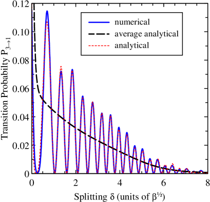
Figure 4: (Color online) Probability for counterintuitive transition $P_{3\rightarrow 1}$ plotted against the energy splitting parameter $\delta$. The other interaction parameters are $\Omega_{12}=\Omega_{23}=\beta^{\frac{1}{2}}$, $T=5\beta^{-\frac{1}{2}}$. The full line shows numerical results, the thin dashed curve the analytical approximation (27) and the thick dashed curve the average probability (29).

V Time evolution in the original Demkov-Osherov model

In the original DO model the time-dependent transition probability from state $\psi_{m}$ to $\psi_{n}$ is given by $P_{m\rightarrow n}(t)=\left|U_{nm}(t,-\infty)\right|^{2}$. We find from Eq. (25) for $t_{i}=-\infty$, $t_{f}=t$ that

$$U_{nm}(t,-\infty)=\sum_{k,l=1}^{3}f_{nk}(t)U_{kl}^{A}(t,-\infty)f_{ml}(-\infty),$$ (35)

and we take into account that

$$\mathsf{F}(-\infty)=\left[\begin{array}[]{ccc}0&-1&0\\ 0&0&1\\ 1&0&0\end{array}\right].$$ (36)

V.1 Counterintuitive transition

By using Eq. (35) we find that the probability of counterintuitive transition $P_{3\rightarrow 1}$ after the crossings reads

$$P_{3\rightarrow 1}(t) = |\sqrt{q_{+}}f_{11}(t)+\sqrt{p_{+}}f_{12}(t)e^{i[\Lambda_{12}(t,\tau)+\phi_{+}]}|^{2}$$ (37a)

$$= \overline{P_{3\rightarrow 1}(t)}+\widetilde{P_{3\rightarrow 1}(t)}$$ (37b)

where

$$\overline{P_{3\rightarrow 1}(t)} =q_{+}f_{11}^{2}+p_{+}f_{12}^{2},$$ (38a)

$$\sim\frac{\Omega_{12}^{2}\left(4\delta^{2}q_{+}+\Omega_{23}^{2}p_{+}\right)}{4\delta^{2}\beta^{2}t^{2}},$$ (38b)

$$\widetilde{P_{3\rightarrow 1}(t)} =2\sqrt{p_{+}q_{+}}f_{11}f_{12}\cos[\Lambda_{12}(t,\tau)+\phi_{+}]$$ (39a)

$$\sim-\frac{\Omega_{12}^{2}\Omega_{23}}{\delta\beta^{2}t^{2}}\sqrt{p_{+}q_{+}}\cos[\Lambda_{12}(t,\tau)+\phi_{+}].$$ (39b)

Figure 5 shows the time evolution of the probability for counterintuitive transition $P_{3\rightarrow 1}$ for three values of the couplings $\Omega_{12}=\Omega_{23}\equiv\Omega$. For these values of $\Omega$ there are almost no oscillations visible, because $p_{+}\ll 1$ in Eq. (39b). The probability $P_{3\rightarrow 1}(t)$ decreases with time, as predicted by Eq. (38), and vanishes for large times towards the DO result $P_{3\rightarrow 1}(\infty)=0$. As predicted, the transition probability $P_{3\rightarrow 1}(t)$ increases with the couplings. The analytical approximation (38) describes very accurately the average probability $\overline{P_{3\rightarrow 1}(t)}$.

V.2 Other transition probabilities

By using Eq. (35) and the large-$t$ asymptotic expansions in Appendix A, we find the leading terms of all average transition probabilities $\overline{P_{m\rightarrow n}(t)}$ after the crossings for equal couplings ($\Omega_{12}=\Omega_{23}\equiv\Omega$),

$$\overline{P_{1\rightarrow 1}(t)} \sim p+\frac{\Omega^{2}}{\beta^{2}t^{2}}\left[\varkappa^{2}(q^{2}-p)-p^{2}\right],$$ (40a)

$$\overline{P_{1\rightarrow 2}(t)} \sim pq+\frac{\Omega^{2}}{\beta^{2}t^{2}}(1-3pq),$$ (40b)

$$\overline{P_{1\rightarrow 3}(t)} \sim q^{2}+\frac{\Omega^{2}}{\beta^{2}t^{2}}\left[q\left(p-q\right)+\varkappa^{2}(p-q^{2})\right],$$ (40c)

$$\overline{P_{2\rightarrow 1}(t)} \sim q+\frac{\Omega^{2}}{\beta^{2}t^{2}}\left(p^{2}-q-\varkappa^{2}q^{2}\right),$$ (40d)

$$\overline{P_{2\rightarrow 2}(t)} \sim p^{2}+\frac{\Omega^{2}}{\beta^{2}t^{2}}(1-3p^{2}),$$ (40e)

$$\overline{P_{2\rightarrow 3}(t)} \sim pq+\frac{\Omega^{2}}{\beta^{2}t^{2}}\left[p(p-q)+\varkappa^{2}q^{2}\right],$$ (40f)

$$\overline{P_{3\rightarrow 1}(t)} \sim \frac{\Omega^{2}}{\beta^{2}t^{2}}\left(\varkappa^{2}p+q\right),$$ (40g)

$$\overline{P_{3\rightarrow 2}(t)} \sim q+\frac{\Omega^{2}}{\beta^{2}t^{2}}(p-2q),$$ (40h)

$$\overline{P_{3\rightarrow 3}(t)} \sim p+\frac{\Omega^{2}}{\beta^{2}t^{2}}\left(q-p-\varkappa^{2}p\right),$$ (40i)

where, as before, $\varkappa^{2}=\Omega^{2}/4\delta^{2}$. All these probabilities have the correct DO limits (5) for $t\rightarrow\infty$. It is interesting to note that the counterintuitive-transition probability in the original DO model (40g) is one-half of the one in the finite DO model (34g).

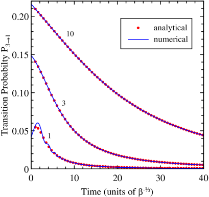
Figure 5: (Color online) Time evolution of the probability for counterintuitive transition $P_{3\rightarrow 1}$ in the original DO model ($t_{i}=-\infty$) for $\delta=\beta^{\frac{1}{2}}$ and three values of the couplings, $\Omega_{12}=\Omega_{23}=\beta^{\frac{1}{2}}$, $3\beta^{\frac{1}{2}}$, and $10\beta^{\frac{1}{2}}$ (denoted near the respective curves). The solid curves show numerical results and the dots show the analytical approximation (38) for the average probability.

VI Experimental implementations

This three-state DO model discussed here can be realized in several physical systems. One example is when a chirped laser pulse couples an initially populated state to a manifold of two levels simultaneously ARPC , the energy diagram for which is identical to the one in Fig. 1, with state $\psi_{2}$ being the initial state. Adiabatic evolution can produce in this system a very selective excitation even if the Fourier bandwidth of the laser pulse is larger than the level spacing within the manifold. Indeed, for red-to-blue chirp ($\beta>0$) the system will follow from left to right the lowest adiabatic energy, which links the initial state $\psi_{2}$ to the lowest diabatic (unperturbed) state $\psi_{1}$ of the manifold. In contrast, for blue-to-red chirp ($\beta<0$) the system would follow (from right to left in Fig. 1) the highest adiabatic energy, linking state $\psi_{2}$ to the highest diabatic state $\psi_{3}$. Therefore, the chirp sign alone determines if the population is directed towards the lowest or the highest state of the manifold. This excitation scheme has been demonstrated experimentally by Warren and co-workers Melinger on the $3s$-$3p$ transition in sodium. Red-to-blue chirped picosecond pulses populated predominantly the lower fine-structure level $3p$ ${}^{2}P_{1/2}$, while blue-to-red chirped pulses placed the population onto the upper fine-structure level $3p$ ${}^{2}P_{3/2}$. Counterintuitive transitions can be demonstrated in this system by using the same setup as described above, but starting in one of the fine-structure levels.

Another example of the model discussed here is Stark-chirped rapid adiabatic passage (SCRAP) SCRAP-theory ; SCRAP-experiment ; SCRAP-3S where level crossings are created by inducing ac Stark shifts of the energy levels by a strong off-resonant laser pulse. A level diagram similar to the one in Fig. 1 is found in the three-state version of SCRAP SCRAP-3S .

It is also worth noting a similarity between the finite DO model presented here and multiple-ground-state models of optical shielding of cold collisions in magneto-optical atom traps Suominen96a ; Suominen96b ; Yurovsky97 ; Napolitano ; Piilo . Optical shielding techniques were originally developed to prevent laser cooled atoms from escaping the trap by making the collisions between the atoms elastic Suominen96b . The experiments show that the shielding process saturates, in contrast to the expected complete shielding, when the intensity of the shielding field is increased Suominen96b . The reason for the saturation is still an open problem and may have a connection to the counterintuitive transitions in the corresponding multiple-ground-state level scheme of the quasimolecule, which in its simple form resembles the present model.

VII Conclusions

We have calculated analytically the probability for the counterintuitive transition $\psi_{3}\rightarrow\psi_{1}$ in a three-state system with crossing energies. We have performed the derivation in the adiabatic basis by assuming instantaneous transitions at the level crossings and adiabatic evolution elsewhere. The counterintuitive transition probability $P_{3\rightarrow 1}$ is nonzero at finite times, whereas it vanishes for infinite coupling duration, thus recovering the result in the DO model. A very good agreement with the numerical results is found. This approach has been used to derive the other transition probabilities within the three-state system too.

Our results suggest that at large $T$ the probability for a counterintuitive transition is proportional to the factor $\Omega^{2}/(\delta^{2}\beta^{2}T^{2})$. The decrease with the interaction duration $T$ is expected as for $T\rightarrow\infty$ the probability should vanish (DO model). The increase with the coupling $\Omega$ is also anticipated since larger interaction is expected to increase weak transitions. The decrease vs the energy splitting $\delta$ between the concerned states $\psi_{1}$ and $\psi_{3}$ is natural too. The decrease vs the slope $\beta$ is more subtle. Since $\beta T$ is the diabatic energy of state $\psi_{2}$, and since states $\psi_{1}$ and $\psi_{3}$ interact with each other via $\psi_{2}$, the effective coupling duration for the transition $\psi_{3}\rightarrow\psi_{1}$ depends on the slope $\beta$: the larger the slope the smaller the duration and therefore the smaller the transition probability. The other (“intuitive”) transition probabilities exhibit similar dependences of the finite-duration corrections on the interaction parameters.

We have described physical examples of coherent atomic excitation where the described counterintuitive transition can be observed. The model studied here resembles also the simple form of the multiple-ground-state quasimolecule model used to study optical shielding in magneto-optical atom traps Suominen96a ; Suominen96b . The saturation of optical shielding in high laser intensities has been earlier attributed to off-resonant excitation to attractive states, counterintuitive transitions or other processes including multiple partial waves Suominen96a ; Suominen96b ; Yurovsky97 . The results here show that the probability for counterintuitive transitions is clearly non-negligible and indicate that they can also play a role in the saturation of optical shielding.

Acknowledgements

This work has been supported by the European Union’s Transfer of Knowledge project CAMEL (Grant No. MTKD-CT-2004-014427), and the Alexander von Humboldt Foundation. AAR acknowledges support from the EU Marie Curie Training Site project HPMT-CT-2001-00294. JP acknowledges support from the Magnus Ehrnrooth Foundation and thanks for the hospitality during his visit to Sofia University.

Appendix A Asymptotics of the eigenvalues and the eigenstates

Here we present the asymptotics of the eigenvalues (8) at large positive time $t>0$, i.e. for $\beta t\gg\delta$ and $\beta t\gg\Omega$. Then $a=-\beta t$, $b=-(\delta^{2}+\Omega_{12}^{2}+\Omega_{23}^{2})$, $c=\delta^{2}\beta t\left[1+\left(\Omega_{12}^{2}-\Omega_{23}^{2}\right)/(\delta\beta t)\right]$, and

$$s \sim \beta t+\frac{3\left(\delta^{2}+\Omega_{12}^{2}+\Omega_{23}^{2}\right)}{2\beta t},$$ (41a)

$$\cos\theta \sim 1-\frac{27\delta^{2}}{2\beta^{2}t^{2}},$$ (41b)

$$\theta \sim \frac{3\sqrt{3}\delta}{\beta t}.$$ (41c)

The eigenvalues have the asymptotics

$$\lambda_{1} \sim \beta t+\frac{\Omega_{12}^{2}+\Omega_{23}^{2}}{\beta t},$$ (42a)

$$\lambda_{2} \sim \delta-\frac{\Omega_{23}^{2}}{\beta t},$$ (42b)

$$\lambda_{3} \sim -\delta-\frac{\Omega_{12}^{2}}{\beta t}.$$ (42c)

Hence we find from Eqs. (10) that

$$\varphi_{1} \sim \left[\frac{\Omega_{12}}{\beta t},\ 1-\frac{\Omega_{12}^{2}+\Omega_{23}^{2}}{2\beta^{2}t^{2}},\ \frac{\Omega_{23}}{\beta t}\right]^{T},$$ (43a)

$$\varphi_{2} \sim \left[-\frac{\Omega_{12}\Omega_{23}}{2\delta\beta t},\ -\frac{\Omega_{23}}{\beta t},\ 1-\frac{\Omega_{23}^{2}(\Omega_{12}^{2}+4\delta^{2})}{8\delta^{2}\beta^{2}t^{2}}\right]^{T},$$ (43b)

$$\varphi_{3} \sim \left[-1+\frac{\Omega_{12}^{2}(\Omega_{23}^{2}+4\delta^{2})}{8\delta^{2}\beta^{2}t^{2}},\ \frac{\Omega_{12}}{\beta t},\ -\frac{\Omega_{12}\Omega_{23}}{2\delta\beta t}\right]^{T}.$$ (43c)

Appendix B Symmetries of the eigenvalues and the eigenstates

The eigenvalues and the eigenstates simplify when $t_{i}=-T$, $t_{f}=T$ and $\Omega_{12}=\Omega_{23}\equiv\Omega$. Then $\alpha_{+}=\alpha_{-}\equiv\alpha$, $p_{+}=p_{-}\equiv p$, $q_{+}=q_{-}\equiv q=1-p$, $a(T)=-\beta T$, $b(T)=-\delta^{2}-2\Omega^{2}$, $c(T)=\delta^{2}\beta T$, and

$$s(T) = \sqrt{\beta^{2}T^{2}+3\delta^{2}+6\Omega^{2}},$$ (44a)

$$\cos\theta(T) = \frac{\beta T}{s^{3}}(\beta^{2}T^{2}-9\delta^{2}+9\Omega^{2}).$$ (44b)

Hence $$\theta(-T)=\pi-\theta(T) \lambda_{1}(-T)=-\lambda_{3}(T) \lambda_{2}(-T)=-\lambda_{2}(T) \lambda_{3}(-T)=-\lambda_{1}(T)$$ and therefore , , , and

$$\Lambda_{2}(-\tau,-T) = \Lambda_{2}(\tau,T)=-\Lambda_{2}(T,\tau),$$ (45a)

$$\Lambda_{2}(T,-T) = \Lambda_{2}(\tau,-\tau)=0,$$ (45b)

$$\Lambda_{1}(-\tau,-T) = \Lambda_{3}(\tau,T)=-\Lambda_{3}(T,\tau),$$ (45c)

$$\Lambda_{3}(-\tau,-T) = \Lambda_{1}(\tau,T)=-\Lambda_{1}(T,\tau).$$ (45d)

The transformation matrix at $$-T$$ is given by

$$\mathsf{F}(-T)=\left[\begin{array}[]{ccc}-f_{33}(T)&-f_{32}(T)&-f_{31}(T)\\ f_{23}(T)&f_{22}(T)&f_{21}(T)\\ -f_{13}(T)&-f_{12}(T)&-f_{11}(T)\end{array}\right].$$ (46)

With these relations taken into account the propagator (23) reduces to Eq. (24).

References

• (1) L.D. Landau, Phys. Z. Sowjetunion 2, 46 (1932); C. Zener, Proc. Roy. Soc. (Lond) A137, 696 (1932); E.C.G. Stückelberg, Helv. Phys. Acta 5, 369 (1932).
• (2) C.E. Carroll and F.T. Hioe, J. Phys. A: Math. Gen. 19, 1151 (1986).
• (3) C.E. Carroll and F.T. Hioe, J. Opt. Soc. Am. B 2, 1355 (1985); J. Phys. A: Math. Gen. 19, 2061 (1986).
• (4) D.A. Harmin, Phys. Rev. A 44, 433 (1991).
• (5) S. Brundobler and V. Elser, J. Phys. A 26, 1211 (1993).
• (6) V.N. Ostrovsky and H. Nakamura, J. Phys. A 30, 6939 (1997).
• (7) Y.N. Demkov and V.N. Ostrovsky, Phys. Rev. A 61, 032705 (2000).
• (8) Y.N. Demkov and V.N. Ostrovsky, J. Phys. B 34, 2419 (2001).
• (9) N.V. Vitanov, T. Halfmann, B.W. Shore and K. Bergmann, Ann. Rev. Phys. Chem. 52, 763 (2001).
• (10) M.-O. Mewes, M.R. Andrews, D.M. Kurn, D.S. Durfee, C.G. Townsend, and W. Ketterle, Phys. Rev. Lett. 78, 582 (1997).
• (11) N.V. Vitanov and K.-A. Suominen, Phys. Rev. A 56, R4377 (1997).
• (12) Y.N. Demkov and V. I. Osherov, Zh. Eksp. Teor. Fiz. 53, 1589 (1967) [Sov. Phys. JETP 26, 916 (1968)].
• (13) Y. Kayanuma and S. Fukuchi, J. Phys. B 18, 4089 (1985).
• (14) Y.N. Demkov and V.N. Ostrovsky, J. Phys. B 28, 403 (1995).
• (15) T. Usuki, Phys. Rev. B 56, 13360 (1997).
• (16) V.N. Ostrovsky and H. Nakamura, Phys. Rev. A 58, 4293 (1998).
• (17) Y.N. Demkov, P.B. Kurasov, and V.N. Ostrovsky, J. Phys. A 28, 4361 (1995).
• (18) V.A. Yurovsky and A. Ben-Reuven, J. Phys. B 31, 1 (1998).
• (19) V.A. Yurovsky and A. Ben-Reuven, Phys. Rev. A 63, 043404 (2001).
• (20) A.V. Shytov, Phys. Rev. A 70, 052708 (2004).
• (21) N.A. Sinitsyn, J. Phys. A: Math. Gen. 37, 10691 (2004).
• (22) M.V. Volkov and V.N. Ostrovsky, J. Phys. B: At. Mol. Opt. Phys. 37, 4069 (2004).
• (23) M.V. Volkov and V.N. Ostrovsky, J. Phys. B: At. Mol. Opt. Phys. 38, 907 (2005).
• (24) R. B. Vrijen, G. M. Lankhuijzen, D. J. Maas, and L. D. Noordam, Comments At. Mol. Phys. 33, 67 (1996); B. Broers, H. B. van Linden van den Heuvell, and L. D. Noordam, Phys. Rev. Lett. 69, 2062 (1992); P. Balling, D. J. Maas, and L. D. Noordam, Phys. Rev. A 50, 4276 (1994); D. J. Maas, D. I. Duncan, A. F. G. van der Meer, W. J. van der Zande, and L. D. Noordam, Chem. Phys. Lett. 270, 45 (1997).
• (25) K.-A. Suominen, K. Burnett, P.S. Julienne, M. Walhout, U. Sterr, C. Orzel, M. Hoogerland, and S.L. Rolston, Phys. Rev. A 53, 1678 (1996).
• (26) K.-A. Suominen, J. Phys. B 29, 5981 (1996); J. Weiner, V.S. Bagnato, S. Zilio, and P.S. Julienne, Rev. Mod. Phys. 71, 1 (1999).
• (27) V.A. Yurovsky and A. Ben-Reuven, Phys. Rev. A 55, 3772 (1997).
• (28) R. Napolitano, J. Weiner, and P.S. Julienne, Phys. Rev. A 55, 1191 (1997).
• (29) J. Piilo and K.-A. Suominen, Phys. Rev. A 66, 013401 (2002).
• (30) J. Karczmarek, J. Wright, P. Corkum, and M. Ivanov, Phys. Rev. Lett. 82, 3420 (1999); D.M. Villeneuve, S.A. Aseyev, P. Dietrich, M. Spanner, M.Y. Ivanov, and P.B. Corkum, Phys. Rev. Lett. 85, 542 (2000); N.V. Vitanov and B. Girard, Phys. Rev. A 69, 033409 (2004).
• (31) L. P. Yatsenko, B. W. Shore, T. Halfmann, K. Bergmann, and A. Vardi, Phys. Rev. A 60, R4237 (1999).
• (32) T. Rickes, L.P. Yatsenko, S. Steuerwald, T. Halfmann, B.W. Shore, N.V. Vitanov and K. Bergmann, J. Chem. Phys. 115, 534-46 (2000).
• (33) A.A. Rangelov, N.V. Vitanov, L.P. Yatsenko, B.W. Shore, T. Halfmann, and K. Bergmann, submitted to Phys. Rev. A.
• (34) R.G. Unanyan, N.V. Vitanov, and K. Bergmann Phys. Rev. Lett. 87, 137902 (2001); R.G. Unanyan, M. Fleischhauer, N.V. Vitanov, and K. Bergmann, Phys. Rev. A 66, 042101 (2002).
• (35) M.S. Child, Molecular Collision Theory (Dover, New York, 1974).
• (36) V.A. Yurovsky, A. Ben-Reuven, P.S. Julienne, and Y.B. Band, J. Phys. B 32, 1845 (1999).
• (37) B.W. Shore, The Theory of Coherent Atomic Excitation (Wiley, New York, 1990).
• (38) N.V. Vitanov, Phys. Rev. A 59, 988 (1999).
• (39) J.S. Melinger, S.R. Gandhi, A. Hariharan, J.X. Tull, and W.S. Warren, Phys. Rev. Lett. 68, 2000 (1992).