A past capture event at Sagittarius A* inferred from the fluorescent X-ray emission of Sagittarius B clouds

Abstract

The fluorescent X-ray emission from neutral iron in the molecular clouds (Sgr B) indicates that the clouds are being irradiated by an external X-ray source. The source is probably associated with the Galactic central black hole (Sgr A*), which triggered a bright outburst one hundred years ago. We suggest that such an outburst could be due to a partial capture of a star by Sgr A*, during which a jet was generated. By constraining the observed flux and the time variability ($\sim$ 10 years) of the Sgr B’s fluorescent emission, we find that the shock produced by the interaction of the jet with the dense interstellar medium represents a plausible candidate for the X-ray source emission.

1 Introduction

The major component in the Galactic center (GC) region is a central molecular zone (Morris & Serabyn 1996), which contains about 10% ($\sim 3\times 10^{7}M_{\odot}$) of the total molecular gas of the Galaxy (Dahmen et al. 1998). The most well-known and massive central molecular clouds are Sagittarius (Sgr) B1 and B2. The central molecular zone is bright in diffuse X-rays (Sunyaev et al. 1993; Koyama et al. 2007a), including thermal and non-thermal emission. The thermal component, whose spectrum contains strong K-shell emission lines from highly ionized atoms, such as Fe XXV (6.7 keV), and S XV (2.45 keV), could be associated with a hot plasma in collisional ionization equilibrium with multiple temperatures. This plasma emission decreases monotonically with an increasing distance from the GC, and extends about over 1 degree in longitude (Koyama et al. 1989; Yamauchi et al. 1990). In contrast, the brightest non-thermal emission line from neutral iron, with a strong K-shell transition line at 6.4 keV, was found to be near the Sgr B region (Koyama et al. 1996). After the first discovery of the 6.4-keV line emission by the ASCA satellite, a much deeper observation of the Sgr B region was provided by the Suzaku satellite (Koyama et al. 2007b). Consequently, some remarkable features in the X-ray spectra were observed, such as: a large equivalent width ($\geq$ 1 keV) of the 6.4-keV line, and a deep iron K-absorption edge at 7.1 keV (equivalent neutral hydrogen column density $\sim 10^{23-24}~{}\rm cm^{-2}$).

These spectral features suggest that the 6.4-keV line, and the underlying continuum emission, could originate from fluorescence and Thomson scattering in the molecular clouds, which are irradiated by an external X-ray source (Koyama et al. 1996; Sunyaev & Churazov 1998). The detailed morphology of the 6.4-keV line emission of Sgr B2 cloud was investigated by Chandra (Murakami et al. 2001). The line exhibits a concave shape (the peak position of the emitting region is located about $1-2$ arcmin from the cloud center), pointing to the GC direction. This strongly suggests that the external source is loacted in the GC direction. However, no sufficiently bright X-ray source has been detected there. Therefore, Koyama et al. (1996, 2007b) and Murakami et al. (2001) proposed that the supermassive black hole (BH), harbored at the GC (Sgr A*), probably triggered a bright outburst about one hundred years ago, which is the delayed time in the light travel due to the reflection by Sgr B2. As an alternative to the above X-ray reflection model, Predehl et al. (2003), Yusef-Zadeh et al. (2007), and Dogiel et al. (2009b) proposed that the origin of the 6.4-keV line and X-ray continuum emission could be due to non-relativistic electrons or protons. However, this model is disfavored by the inferred metal abundances of the hot plasma in the GC region (Nobukawa et al. 2010), even that this conclusion cannot be applied to the case of protons, because their estimated abundance depends strongly on the spectral index of the protons (see Dogiel et al. 2010). The most convincing evidence that supports the X-ray reflection model comes from the detection of a similar pattern of emission variability in causally disconnected regions (Inui et al. 2009). This pattern was recently confirmed by the observation of a clear decay, of about 40% during the past 7 years, of the hard X-ray continuum emission from Sgr B2 (Terrier et al. 2010). As reported by Ponti et al. (2010), such a time variability can also be found in other molecular clouds (e.g., G 0.11-0.11). In particular, Ponti et al. (2010) observed an apparent superluminal motion of a light front illuminating a molecular nebula, which cannot be due to low energy cosmic rays, or to a source located inside the cloud.

In this paper, we use the X-ray reflection model, and suggest that the required past outburst could be due to a partial capture of a star by Sgr A*. During the accretion of the stellar matter onto the BH, an accompanying jet could be generated, as seen in some accreting systems, such as microquasars (e.g. Gallo et al. 2003; Fender 2003; Fender & Maccarone 2004). Then, by considering the deceleration of the jet by the dense interstellar medium, the resulting shock emission could become a plausible X-ray source, which is responsible for the fluorescent emission from the Sgr B region. Such a (partial or full) stellar capture event by a central supermassive BH has perhaps already been observed in some flaring “normal” galaxies (e.g., Renzini et al. 1995; Li et al. 2002; Donley et al. 2002). In our Galaxy, as suggested by Cheng et al. (2006), stellar captures may also be required to provide a positron source for the observed electron-positron annihilation emission from the GC region. Meanwhile, in such a stellar capture scenario, the diffuse hard X-ray and gamma-ray emission from the GC region can also be explained well (Cheng et al. 2007; Dogiel et al. 2009a,b,c,d).

The present paper is organized as follows. In Section 2, by using the X-ray reflection model, we derive from the observed 6.4-keV line luminosity the X-ray luminosity of the external source. In Section 3, we briefly describe the tidal capture process. In Section 4, we investigate the dynamics and the synchrotron radiation of the shock produced by the deceleration of the jet. Then, some basic properties of the jet are inferred from the observations. Finally, we discuss and conclude our results in Section 5.

2 The X-ray reflection model

In the following we specifically refer to Sgr B2 cloud as M $0.66-0.02$ (Inui et al. 2009), and a radius of $r_{B}\sim$3.2 arcmin is adopted for this object. The distance to Sgr B2 is $d_{B}\approx 7.8^{+0.8}_{-0.7}$ kpc (Reid et al. 2009), and consequently $r_{B}\approx 7.3$ pc. Due to their projected offset $\sim 0.09$ kpc and to the offset along the light of sight, $\sim 0.13$ kpc, the distance $d_{AB}$ between Sgr B2 and Sgr A* is about $\sim 0.16$ kpc (Reid et al. 2009). Denoting the (isotropically-equivalent) X-ray luminosity of Sgr A* by $\mathcal{L}_{A,X}$, and the luminosity of the 6.4-keV line emission from Sgr B2 by $\mathcal{L}_{B,6.4}$, respectively, their ratio can be roughly estimated as (Murakami et al. 2000)

$$\Re \equiv {\mathcal{L}_{B,\rm 6.4}\over\mathcal{L}_{A,X}}$$ (1)

$$= {1\over 4}\left({r_{B}\over d_{AB}}\right)^{2}e^{-\sigma(\geq 7.1)N_{\rm H,c}}\left(1-e^{-0.34\sigma_{\rm Fe}Z_{\rm Fe}N_{\rm H,c}}\right)$$

$$\times e^{-\sigma(6.4)N_{\rm H,G}}\approx 7.0\times 10^{-6},$$

where the reflection is assumed to be isotropic. In Eq. (1) $\sigma(E)$ is the photoelectric absorption cross section per hydrogen atom for standard interstellar matter ($\sigma(\geq 7.1)\approx 2.4\times 10^{-24}\rm~{}cm^{2}$ and $\sigma(6.4)\approx 1.3\times 10^{-24}\rm~{}cm^{2}$ (Morrison & McCammon 1983)), $\sigma_{\rm Fe}\approx 3.7\times 10^{-20}\rm~{}cm^{2}$ (for $E\geq 7.1$ keV) is the photoelectric absorption cross section of an iron atom (Rakavy & Ron 1967), the factor $0.34$ is the fluorescence probability, and $Z_{\rm Fe}\approx 1.6Z_{\rm Fe,\odot}\approx 10^{-5}$ is the abundance of iron (Nobukawa et al. 2010). The Galactic absorption from the cloud to the observer is assumed to be $N_{\rm H,G}\approx 6\times 10^{22}\rm~{}H~{}cm^{-2}$ (Sakano et al. 1997), and from the intensity of the CS emission, which is directly correlated with the cloud mass, the column density of the Sgr B2 cloud can be inferred to be $N_{\rm H,c}\approx 8\times 10^{23}~{}\rm H~{}cm^{-2}$ (Tsuboi et al. 1999; Ponti et al. 2010). The interstellar absorption from Sgr A* to the cloud is neglected. An improved model for the calculation of $\Re$ can be found in Murakami et al. (2000).

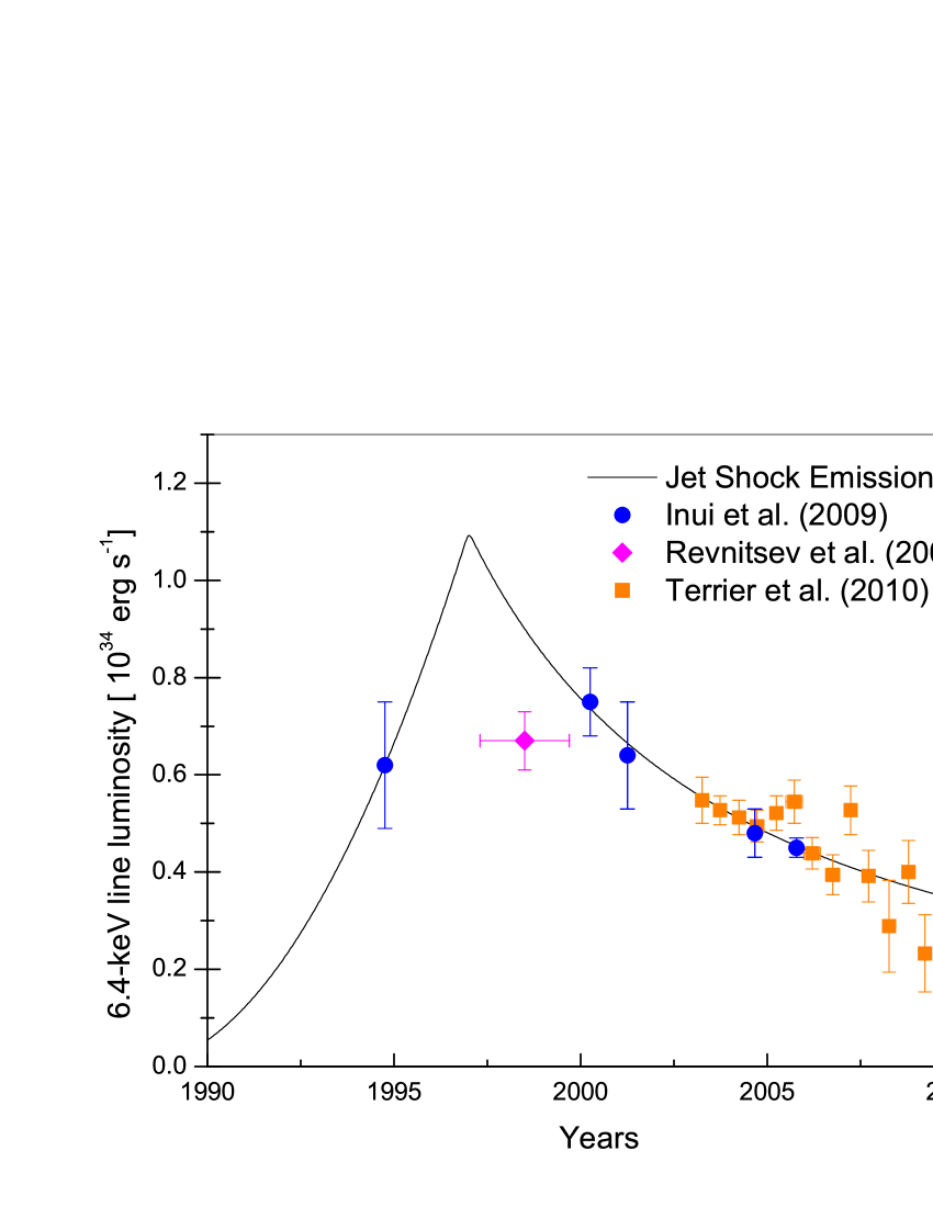
Figure 1: The observational luminosity data of the 6.4-keV line emission from Sgr B2 cloud and an illustrative fitting (solid line) by using Equation (23). The fitting parameters are $t_{0}=1988$, $T_{\rm d}=9$ yr, and $\Re\mathcal{L}_{\rm sh,X,d}=1.1\times 10^{34}\rm~{}erg~{}s^{-1}$.

There have been several deep exposure and short survey observations of the Sgr B2 cloud with different satellites or instruments, such as ASCA, XMM-Newton, BeppoSAX, Chandra, Suzaku, and INTEGRAL. Some observational fluxes of the 6.4-keV line emission can be found from the literatures (e.g., Revnivtsev et al. (2004) and Inui et al. (2009)). They are of the order of magnitude of $\sim 10^{-4}~{}\rm photons~{}s^{-1}~{}cm^{-2}$. With a distance $d_{B}\approx 7.8^{+0.8}_{-0.7}$ kpc, the luminosity $\mathcal{L}_{B,6.4}$ can be calculated to be around $\sim 10^{34}~{}\rm erg~{}s^{-1}$. The specific observational data are shown in Figure 1. Combining this result with equation Eq. (1), we can estimate the order of magnitude of the luminosity of the source as

$$\mathcal{L}_{A,X}={\mathcal{L}_{B,6.4}\over\Re}\sim 10^{39}~{}\rm erg~{}s^{-1},$$ (2)

which is much higher than the present luminosity of Sgr A*, which is of the order of $\sim 10^{33-35}\rm~{}erg~{}s^{-1}$ (Baganoff et al. 2003). Fig. 1 also shows some 6.4-keV line emission data, extrapolated from the $20-60$ keV continuum emission data from Terrier et al. (2010), by assuming that both the 6.4-keV line and the continuum emissions have the same trend, and that the different sets of 6.4-keV line emission data should be joined continuously. The apparent time variation exhibited by the data indicates that the source emission is likely to be a transient. This implies that about one hundred years ago a bright outburst had happened at Sgr A*. The moment of the outburst can be obtained from the delay in the light travel time, due to the reflection by Sgr B2, given by ${\rm\sim(0.16~{}kpc-0.13~{}kpc)}/c$ .

3 Stellar tidal capture by Sgr A*

Observations show that at the center of Sgr A* there is a supermassive BH , with a mass of $4\times 10^{6}~{}M_{\odot}$ (see the review by Genzel & Karas 2007). In the close vicinity of Sgr A* (less than 0.04 pc from it), about 35 low-mass stars ($1-3~{}M_{\odot}$) and about 10 massive stars ($3-15~{}M_{\odot}$) are present (see Alexander & Livio 2004). Hence, the past outburst probably indicates a (partial) capture of a star by Sgr A*. When a star gets very close to a supermassive BH, it will experience tidal distortions, and even disruptions. The strength of a tidal encounter can be defined by the square root of the ratio between the surface gravity and the tidal acceleration at the pericenter,

$$\eta=\left({R_{p}^{3}\over GM_{\bullet}R_{\star}}{GM_{\star}\over R_{\star}^{2}}\right)^{1/2},$$ (3)

where $G$, $R_{p}$, $M_{\star}$, $R_{\star}$, $M_{\bullet}$ are Newton’s constant, the pericentric distance, the stellar mass, the stellar radius, and the BH’s mass, respectively. If $M_{\bullet}>10^{8}~{}M_{\odot}$, and for a sufficiently small $R_{p}$, the star would directly fall into the BH’s event horizon, without emitting any significant amount of energy. However, for a BH such as Sgr A*, the star would disrupt when $\eta<1$, which corresponds to

$$R_{p} < R_{T}=R_{\star}\left({M_{\bullet}\over M_{\star}}\right)^{1/3}$$ (4)

$$= 7.0\times 10^{12}{~{}\rm cm}~{}\left({M_{\bullet}\over 10^{6}M_{\odot}}\right)^{1/3}\left({M_{\star}\over M_{\odot}}\right)^{-1/3}\left({R_{\star}\over R_{\odot}}\right),$$

where $R_{T}$ is called the tidal radius. On the other hand, for somewhat larger pericentric separations ($\eta>1$), the star avoids total disruption, but it may lose parts of its envelope, which are captured by the BH. The stripped star, having positive energy, escapes from the system. We denote the capture fraction of the total stellar mass by $\xi$.

After the disruption or stripping, the bound material follows a highly eccentric orbit, and after completing one orbit it returns to the central BH. A circular transient accretion disk forms, producing a transient black body emission. The emission reaches a peak when most of the material first returns to the pericenter, after a time $1.5~{}t_{\min}$, where (Ulmer 1999)

$$t_{\min} = {2\pi R_{p}^{3}\over(GM_{\bullet})^{1/2}(2R_{\star})^{3/2}}$$ (5)

$$= 0.1~{}{\rm yr}~{}\left({R_{p}\over R_{T}}\right)^{3}\left({M_{\rm BH}\over 10^{6}M_{\odot}}\right)^{1/2}\left({M_{\star}\over M_{\odot}}\right)^{-1}\left({R_{\star}\over R_{\odot}}\right)^{3/2}.$$

We can use this timescale to estimate the accretion rate, and the corresponding bolometric luminosity of the disk, as $\dot{M}=(2\xi M_{\star}/3t_{\min})(t/t_{\min})^{-5/3}$, and $\mathcal{L}_{\rm disk}=\epsilon\dot{M}c^{2}$, respectively, where $\epsilon$ is the radiation efficiency, which is usually taken to be $\sim$10%. However, for an accretion rate much lower than the Eddington rate, the accretion flow is likely to be radiatively inefficient (e.g., Yuan, Quataert & Narayan 2003). In this case most of the thermal energy released by viscosity, and increased by compression, will be retained in the gas, and advected to the BH. Therefore we could have a very small $\epsilon\ll$10%. Moreover, since the frequency with which a solar type star passes within a distance $R_{T}$ is about $10^{-4}-10^{-5}\rm~{}yr^{-1}$ (Rees 1988), the capture event that happened one hundred years ago is quite unlikely to be a full capture, i.e., $\xi\ll 1$.

Therefore the peak value of the disk luminosity can be estimated as (Ulmer 1999)

$$\mathcal{L}_{\rm disk,p} = 3.4\times 10^{44}~{}{\rm erg~{}s^{-1}}~{}\left({\epsilon\over 0.01}\right)\left({\xi\over 0.1}\right)\left({R_{p}\over R_{T}}\right)^{-3}$$ (6)

$$\times\left({M_{\bullet}\over 10^{6}M_{\odot}}\right)^{-1/2}\left({M_{\star}\over M_{\odot}}\right)^{2}\left({R_{\star}\over R_{\odot}}\right)^{-3/2}.$$

Since this bolometric luminosity is very high, the disk emission could be an appropriate source for the X-ray echo emission of Sgr B2. Unfortunately, most of the disk energy will be actually released into an energy band much lower than hard X-rays, as can be seen in some stellar-capture-like flares, found in UV/optical detections (e.g., Gezari et al. 2008, 2009). Moreover, a UV flare detected at the center of a mildly active elliptical galaxy, NGC 4552, even indicates a candidate for a partial capture event (Renzini et al. 1995). Theoretically, we can also give an upper limit for the disk temperature associated with an Eddington luminosity, $\mathcal{L}_{E}=1.5\times 10^{38}{\rm erg~{}s^{-1}}(M_{\bullet}/M_{\odot})$, emitted from the tidal radius (Ulmer 1999),

$$T_{\rm eff} = \left({\mathcal{L}_{E}\over 4\pi R_{T}^{2}\sigma}\right)^{1/4}$$ (7)

$$= 22~{}{\rm eV}~{}\left({M_{\bullet}\over 10^{6}M_{\odot}}\right)^{1/12}\left({M_{\star}\over M_{\odot}}\right)^{1/6}\left({R_{\star}\over R_{\odot}}\right)^{-1/2}$$

or from the Schwarzschild radius (Ulmer 1999),

$$T_{\rm eff}=\left[{\mathcal{L}_{E}\over 4\pi(5R_{s})^{2}\sigma}\right]^{1/4}=48~{}{\rm eV}~{}\left({M_{\bullet}\over 10^{6}M_{\odot}}\right)^{-1/4},$$ (8)

where we have neglected a factor of the order of unity. The above equations may underestimate the real temperature in the disk, but the luminosity in the partial capture is also lower than the Eddington luminosity. Therefore, it seems difficult for the disk emission to provide sufficient X-ray photons with energy $>7.1$ keV to excite the strong 6.4-keV line emission of the clouds.

The strong UV emission can still influence the environment of Sgr A*. Taking Sgr B2 as an example, we can estimate the mean free path of a UV photon with energy $\varepsilon_{\rm UV}\sim k_{B}T_{\rm eff}\sim 20$ eV in the cloud as $l=(\sigma_{a}n_{H})^{-1}=2.3\times 10^{13}$cm, where the number density of neutral hydrogens is $n_{H}\sim N_{H,c}/(2r_{B})=1.8\times 10^{4}~{}\rm cm^{-3}$, and the photoionization absorption cross section can be expressed as $\sigma_{a}\approx 2.5\times 10^{-18}(\varepsilon_{\rm UV}/20\rm eV)^{-3}$ (Lang 1980). This indicates that if the layer is so hot that it can be fully ionized, the UV photons can only penetrate into a very thin surface layer of the cloud. In view of the small thermal capacity of the layer, $\sim 10^{41}\rm erg~{}K^{-1}$, it is indeed very easy to heat the layer to high temperatures, as long as a small fraction of the UV energy is converted into thermal energy. For example, the ionized electrons can lose their kinetic energy to heat the plasma. After being continuously irradiated by the UV flare for a few months, the total mass of the fully ionized envelope of the cloud, exposed to Sgr A*, can be estimated as $M_{\rm ion}\sim{N_{UV}}\left({r_{B}^{2}/4d_{AB}^{2}}\right)m_{H}=25M_{\odot}$, where $N_{UV}\sim(1.5L_{\rm disk,p}t_{\rm min}/\varepsilon_{\rm UV})$ is the total number of the photons, $m_{H}$ is the mass of hydrogen atom, and we assume that each UV photon ionizes one hydrogen atom. Consequently, the width of the ionized envelope is about $\Delta\sim M_{\rm ion}/(2\pi r_{B}^{2}n_{H}m_{H})=5.2\times 10^{14}{\rm cm}=23~{}l$, which means that only an extremely small fraction $\Delta/r_{B}=2.3\times 10^{-5}$ of the cloud can be ionized by the UV flare. Finally, due to the high temperature of the ionized region, the ionized material may be able to ultimately evaporate from the cloud and mix with the surrounding plasmas.

What can be the appropriate X-ray source in this stellar-partial-capture model? Similarly to the active galactic nuclei, one may suggest that the Compton up-scattering of the soft disk photons by a hot corona can produce strong hard X-ray emission. This is a reasonable scenario, but unfortunately it is not clear when and how a hot corona can be formed, and even whether there will be a corona, since the disk is very short-lived and strongly time-dependent. Even if a corona accompanying the disk can indeed be formed, the temporal behavior of the corona emission still should basically follow the behavior of the disk emission, whose variability timescale (see Eq. 6) is however much shorter than 10 years. Alternatively, as suggested by Cheng et al. (2006), a jet could be generated during the capture event. This can be suggested from the fact that accreting BHs in microquasars sometimes are accompanied by jet emission. Although in the high/soft state of microquasars the jet formation is highly suppressed (Fender et al. 1999; Gallo et al. 2003), the evidences for jet emission are solid enough in the low state (e.g. Gallo et al. 2003) and in the “very high” state (e.g. Fender 2003; Fender & Maccarone 2004). Therefore, we suggest that the source emission could be produced by the jet.

4 Shock emission arising from the jet deceleration

If a jet was indeed ejected during the past capture event, a shock would be produced from the interaction of the jet outflow with the interstellar medium. Using such a jet shock emission, Wong et al. (2007) explained the transient X-ray and optical data from some nearby normal galactic nuclei, where a capture event may had also occurred. Due to the motion of the jet outflow, the ambient interstellar medium is gradually swept up by the shock, and simultaneously the outflow is decelerated. We denote the deceleration timescale of the outflow by $T_{\rm d}$. Before $T_{\rm d}$, the outflow coasts, and due to the accumulation of the shocked medium the emission of the shock increases. After $T_{\rm d}$, the emission is weakened due to the significant deceleration of the outflow. In other words, the shock emission would arrive at the peak at around $T_{\rm d}$, and the increasing time of the emission roughly reflects the deceleration timescale of the outflow (see Equation (23)). Therefore, according to the observational data, shown in Fig. 1, it seems acceptable to take decades as a fiducial value for $T_{\rm d}$.

Hence we can use $T_{\rm d}\sim 10$ yr to find out whether initially the outflow moves at a relativistic or non-relativistic velocity. For an outflow with an isotropically-equivalent energy $\mathcal{E}$, we first define a critical mass as $\mathcal{M}_{\rm of,c}=\mathcal{E}/c^{2}=5.6\times 10^{-5}M_{\odot}~{}\mathcal{E}_{50}$. Hereafter, the convention $Q_{x}=Q/10^{x}$ is adopted in cgs units, except for the mass that is expressed in units of $M_{\odot}$. Obviously, if the mass of the outflow $\mathcal{M}_{\rm of}<\mathcal{M}_{\rm of,c}$, the outflow has initially a relativistic velocity, with a Lorentz factor of $\Gamma_{i}=\mathcal{E}/(\mathcal{M}_{\rm of}c^{2})$. In this case, the deceleration time can be defined as $\Gamma_{i}^{2}\mathcal{M}_{\rm sw,d}c^{2}=\mathcal{E}$ with $\mathcal{M}_{\rm sw,d}={4\over 3}\pi R_{\rm d}^{3}nm_{p}$ and $R_{\rm d}=2\Gamma_{i}^{2}cT_{\rm d}$, where $n$ is the number density of the ambient medium, $\mathcal{M}_{\rm sw}$ is the total mass of the swept-up medium, $R$ is the radius of the shock, $m_{p}$ is the mass of proton, and $c$ is the speed of light. The above equations yield

$$T_{\rm d}=\left({3\mathcal{E}\over 32\pi nm_{p}c^{5}\Gamma_{i}^{8}}\right)^{1/3}=2.0\times 10^{4}{\rm~{}s}~{}\mathcal{E}_{50}^{-7/3}\mathcal{M}_{\rm of,-5}^{8/3}n_{1}^{-1/3},$$ (9)

where we take $n\sim 10~{}\rm cm^{-3}$ as a fiducial value. On the other hand, if $\mathcal{M}_{\rm of}>\mathcal{M}_{\rm of,c}$, the outflow would be non-relativistic, with a velocity of $V_{i}=(2\mathcal{E}/\mathcal{M}_{\rm of})^{1/2}$. In this case, we can obtain $T_{\rm d}$ from the equations ${1\over 2}\mathcal{M}_{\rm sw,d}V_{i}^{2}=\mathcal{E},~{}\mathcal{M}_{\rm sw,d}={4\over 3}\pi R_{\rm d}^{3}nm_{p}$, and $R_{\rm d}=V_{i}T_{\rm d}$, respectively, as

$$T_{\rm d}=\left({3\mathcal{E}\over 2\pi nm_{p}V_{i}^{5}}\right)^{1/3}=1.4\times 10^{9}{\rm~{}s}~{}\mathcal{E}_{50}^{-1/2}\mathcal{M}_{\rm of,-1}^{5/6}n_{1}^{-1/3}.$$ (10)

For $T_{\rm d}\sim 10{~{}\rm yr}$, the relativistic case requires

$$\mathcal{E}>4.3\times 10^{56}{\rm~{}erg}~{}n_{1}T_{\rm d,8.5}^{3},$$ (11)

a condition which is physically unacceptable. In contrast, the non-relativistic case yields a more reasonable result,

$$V_{i}(\mathcal{E}) = 2.5\times 10^{9}~{}{\rm cm~{}s^{-1}}~{}\mathcal{E}_{50}^{1/5}n_{1}^{-1/5}T_{\rm d,8.5}^{-3/5},$$ (12)

$$\mathcal{M}_{\rm of}(\mathcal{E}) = 1.7\times 10^{-2}~{}M_{\odot}~{}\mathcal{E}_{50}^{3/5}n_{1}^{2/5}T_{\rm d,8.5}^{6/5},$$ (13)

which is only mildly dependent on the uncertain model parameter $\mathcal{E}$.

The dynamic evolution of the non-relativistic adiabatic shock is determined by the energy conservation law ${1\over 2}\mathcal{M}_{\rm sw}V^{2}=\mathcal{E}$, which gives

$$V(t)=V_{i}\left\{\begin{array}[]{ll}\tilde{t}^{0},&\tilde{t}<1,\\ \tilde{t}^{-3/5},&\tilde{t}>1\end{array}\right.,$$ (14)

where $\tilde{t}\equiv(t-t_{0})/T_{\rm d}$, with $t_{0}$ being the initial time of the capture event. The deceleration timescale $T_{\rm d}$ is defined by Eq. (10). This is the well-known Sedov solution (Sedov 1969). When the shock propagates through the medium, the energy density behind the shock is given by (Lang 1980)

$$e={9\over 8}nm_{p}V^{2}.$$ (15)

By assuming that a fraction $\epsilon_{B}$ of the internal energy is in form of magnetic energy, the magnetic field strength can be estimated as $B=(8\pi\epsilon_{B}e)^{1/2}$. The shock-accelerated electrons are assumed to have a power-law distribution of the kinetic energy $(\gamma-1)m_{e}c^{2}$, with a minimum Lorentz factor $\gamma_{m}$ given by (Huang & Cheng 2003)

$${dN_{e}\over d\bar{\gamma}}\propto{\bar{\gamma}}^{-p}, ~{}{\rm for~{}}\bar{\gamma}\geq\bar{\gamma}_{m},$$ (16)

where for simplicity $\bar{\gamma}\equiv\gamma-1$ is defined as an effective Lorentz factor, and $p\simeq 2.2$ is the spectral index (Gallant et al. 2002). If the internal energy of the electrons is a small fraction $\epsilon_{e}\sim 0.1$ of the total internal energy (smaller than that of the protons), we can obtain the value of $\bar{\gamma}_{m}$ as (Dai & Lu 2001)

$$\bar{\gamma}_{m}={9\over 32}\epsilon_{e}{p-2\over p-1}{m_{p}\over m_{e}}\left(V\over c\right)^{2}=\bar{\gamma}_{m,\rm d}\left\{\begin{array}[]{ll}\tilde{t}^{0},&\tilde{t}<1,\\ \tilde{t}^{-6/5},&\tilde{t}>1\end{array}\right.,$$ (17)

where $\bar{\gamma}_{m,\rm d}=0.06~{}\epsilon_{e,-1}\mathcal{E}_{50}^{2/5}n_{1}^{-2/5}T_{\rm d,8.5}^{-6/5}$. Considering the synchrotron cooling of the electrons with power $P(\gamma)={4\over 3}\sigma_{T}c(\gamma^{2}-1){B^{2}\over 8\pi}$, a critical cooling Lorentz factor can be determined by $\bar{\gamma}m_{e}c^{2}=P(\gamma)t$ to be

$$\gamma_{c}={6\pi m_{e}c\over\sigma_{T}B^{2}t}=\gamma_{c,\rm d}\left\{\begin{array}[]{ll}\tilde{t}^{-1},&\tilde{t}<1,\\ \tilde{t}^{1/5},&\tilde{t}>1\end{array}\right.,$$ (18)

where $\gamma_{c,\rm d}=8.5\times 10^{3}~{}\epsilon_{B,-1}^{-1}\mathcal{E}_{50}^{-2/5}n_{1}^{-3/5}T_{\rm d,8.5}^{1/5}\gg 1$. Within the time $t$ an electron with an initial Lorentz factor $\gamma>\gamma_{c}$ would quickly cool down below $\gamma_{c}$. Therefore, the spectral index of the net electron distribution above $\gamma_{c}$ becomes $p+1$, and a radiation spectrum of the form $\nu^{-p/2}$ can be produced by these radiative electrons (Sari et al. 1998).

The peak spectral power of an electron can be obtained from the ratio of the total power and of the synchrotron characteristic frequency (Sari et al. 1998)

$$P_{\nu,\max}\approx{P(\gamma)\over\nu(\gamma)}={\sigma_{T}m_{e}c^{2}\over 3q}B\beta^{2}.$$ (19)

$P_{\nu,\max}$ is independent of $\gamma$. Then, for $\nu>\nu_{c}$, the normalized radiation spectrum can be written as

$$\mathcal{L}_{\rm sh}=\nu{N_{e,>\gamma_{c}}P_{\nu,\max}}\left({\nu\over\nu_{c}}\right)^{-p/2},$$ (20)

where the characteristic frequency, corresponding to the $\gamma_{c}$-electrons, is given by

$$\nu_{c}={q\over 2\pi m_{e}c}B\gamma_{c}^{2}=\nu_{c,\rm d}\left\{\begin{array}[]{ll}\tilde{t}^{-2},&\tilde{t}<1,\\ \tilde{t}^{-1/5},&\tilde{t}>1.\end{array}\right.$$ (21)

where $\nu_{c,\rm d}=3.5\times 10^{12}~{}{\rm Hz}~{}\epsilon_{B,-1}^{-3/2}\mathcal{E}_{50}^{-3/5}n_{1}^{-9/10}T_{\rm d,8.5}^{-1/5}\ll\nu_{X}\sim 10^{18}$ Hz. The spectral index $p/2$ is perfectly consistent with the observational index (Terrier et al. 2010). The number of the electrons above $\gamma_{c}$ can be obtained as

$$N_{e,>\gamma_{c}}={4\over 3}\pi R^{3}n\left({\bar{\gamma}_{c}\over\bar{\gamma}_{m}}\right)^{-(p-1)}.$$ (22)

For a fixed frequency $\nu_{X}\sim 10^{18}$ Hz, Eq.  (20) gives the evolution of the X-ray luminosity as

$$\mathcal{L}_{\rm sh,X}=\mathcal{L}_{\rm sh,X,d}\times\left\{\begin{array}[]{ll}\tilde{t}^{2},&\tilde{t}<1,\\ \tilde{t}^{-(3p-4)/2},&\tilde{t}>1\end{array}\right.,$$ (23)

where the peak value at $T_{\rm d}$ is

$$\mathcal{L}_{\rm sh,X,d} = 7.8\times 10^{37}{~{}\rm erg~{}s^{-1}}~{}\epsilon_{e,-1}^{p-1}\epsilon_{B,-1}^{(p-2)/4}$$ (24)

$$\times\mathcal{E}_{50}^{p/2}n_{1}^{(2-p)/4}\nu_{X,18}^{(2-p)/2}T_{\rm d,8.5}^{(4-3p)/2}.$$

The fitting to the observational data, obtained by using Eq. (23), is shown by the solid line in Fig. 1, where $\mathcal{L}_{\rm sh,X,d}=(1.1\times 10^{34}/\Re)~{}\rm erg~{}s^{-1}$. The confrontation between the model and the observations shows that most of the data can be well explained by this simple jet shock emission model. Only the BeppoSAX data (diamond) do not fit with the fitting line.

Taking into account that the jet may be concentrated within a narrow cone, we introduce a beaming factor $f_{b}$, and denote the beaming-corrected energy of the jet by $E_{\rm jet}$. Then we can solve the equation $f_{b}\mathcal{L}_{\rm sh,X,d}(\mathcal{E})=\mathcal{L}_{A,X,\rm peak}\sim 10^{39}~{}\rm erg~{}s^{-1}$ with $\mathcal{E}=E_{\rm jet}/f_{b}$ to obtain

$$E_{\rm jet} = 0.8\times 10^{51}{\rm erg}~{}f_{b,-1}^{(p-2)/p}\epsilon_{e,-1}^{2(1-p)/p}\epsilon_{B,-1}^{(2-p)/2p}$$ (25)

$$\times\mathcal{L}_{A,X,\rm peak,39}^{2/p}n_{1}^{(p-2)/2p}\nu_{18}^{(p-2)/p}T_{\rm d,8.5}^{(3p-4)/p},$$

where the emission from the beamed jet is assumed to be isotropic. Moreover, substituting $\mathcal{E}=E_{\rm jet}/f_{b}$ into Eqs.  (12) and (13), we further obtain

$$V_{i} = 6.0\times 10^{9}{\rm cm~{}s^{-1}}~{}f_{b,-1}^{-2/5p},$$ (26)

$$M_{\rm jet} = f_{b}\mathcal{M}_{\rm of}=0.02~{}M_{\odot}~{}f_{b,-1}^{(5p-6)/5p},$$ (27)

where $\epsilon_{e,-1}=\epsilon_{B,-1}=\mathcal{L}_{A,X,\rm peak,39}=n_{1}=\nu_{X,18}=T_{\rm d,8.5}=1$. By assuming that a fraction $\zeta$ (typically $1-10$%; Yuan et al. 2005) of the total accreted stellar matter can be ejected into the jet, the mass loss of the star can be estimated to be $\sim 0.2~{}M_{\odot}~{}f_{b,-1}^{(5p-6)/5p}\zeta_{-1}^{-1}$, which can be reduced if the jet emission is anisotropic. All of the above results show that one can choose the jet as the hard X-ray source.

It should be noticed that the above analytical calculations are some rough approximations. For example, the realistic transition in the light curve from the increasing phase to the decreasing phase would be much smoother. In this case the BeppoSAX data could be understood. Moreover, we do not consider the sideway expansion of the jet. If we take ${c_{s}={1\over 4}V_{i}}$ as the upper limit of the sound speed of the shocked medium, the timescale of the sideway expansion of the jet can be estimated as $2\sqrt{f_{b}}R_{d}/c_{s}\sim 2T_{d}$. This timescale indicates that about few decades later the jet will become nearly isotropic diffuse material, which will appear as a new component of the environment of Sgr A*, within a region of a few tens of arcseconds. Hence, it is nearly impossible to image the jet one hundred years after the capture event. Nevertheless, on much longer timescales, the interaction of these BH-ejected diffuse materials with the initial diffuse surrounding medium could still play an important role in the GC diffuse X-ray, gamma-ray, 511 keV annihilation line emissions, and in the heating of the surrounding plasma, which had been thoroughly studied in Cheng et al. (2006, 2007) and Dogiel et al. (2009a, b, c).

In addition to Sgr B2, the jet emission can, at least in principle, also influence the other molecular clouds around Sgr A*, but such an influence mostly depends on the distances between the clouds and Sgr A*. Consequently, some clouds reflect the increasing emission, while some others reflect the decreasing emission. More importantly, the emission from the beamed jet is probably highly anisotropic, at least during the first decades, although for simplicity the isotropic approximation is adopted in our calculations. So the reflection by different clouds could be strongly dependent on their viewing angles with respect to the direction of motion of the jet. In addition, the different properties and environments of the different clouds, can also lead to a great diversity of the reflection emission. To a certain extent, Sgr B2 could have a very particular position, just in front of the jet. The distance of the cloud to Sgr A* makes it possible to detect both the increasing and the decreasing emission phases.

5 Conclusion and discussion

In the framework of the X-ray reflection model for the 6.4-keV line emission from Sgr B, we propose that the external X-ray source could be associated with a stellar partial capture event at Sgr A*. A qualitative comparison between the observational and theoretical timescales and luminosities further shows that the source emission is likely to be produced by the shock produced by the jet deceleration (but not by the accretion disk). The inferred energy, mass, and velocity of the jet show that (i) the jet has a low-energy ($\sim 10^{51}\rm erg$), and it is non-relativistic ($\sim 0.1c$) and (ii) the star could be only partially stripped, rather than totally disrupted, corresponding to a capture fraction of $\xi\sim 0.2~{}M_{\star,0}^{-1}f_{b,-1}^{(5p-6)/5p}\zeta_{-1}^{-1}$.

It has been suggested for a long time that supermassive BHs in relatively low luminosity active galactic nuclei can be fed by the tidal capture of stars. However, direct observational evidence for such capture processes is lacking. The investigation in this paper shows that, in view of the short distance to the GC, it may be worthwhile and feasible to carefully observe the GC region to find clues to some historical capture events, even though now Sgr A* is quiescent, with an X-ray luminosity of only $\sim 10^{33-34}\rm~{}erg~{}s^{-1}$ (Baganoff et al. 2003).

Finally, we would like to point out some alternative scenarios for the X-ray source, e.g., (i) Fryer et al. (2006) suggested that the X-ray source could be due to a supernova shock hitting the $50\rm km~{}s^{-1}$ molecular cloud behind, and to the east, of Sgr A*. The last vestige of this interaction is visible now as Sgr A East; (ii) Cuadra et al. (2008) found that shocks produced by stellar winds can create cold clumps of gas, the accretion of which onto Sgr A* would produce for a decade intervals of activity with luminosity as high as $10^{39}~{}\rm erg~{}s^{-1}$. The wind-clump-capture model may have some similarities to our stellar-partial-capture model. But in the present paper we have considered a more detailed analysis of the physical processes after the matter capture by the black hole, and which could be directly responsible for the X-ray emission.

References

- [1] Alexander, T. 2005, Phys. Rept. 419, 65
- [2] Alexander, T. & Livio, M., 2001, ApJ, 560, L143
- [3] Alexander, T., & Livio, M. 2004, ApJ, 606, 21
- [4] Baganoff, F. K., Maeda, Y., Morris, M., et al. 2003, ApJ, 591, 891
- [5] Blandford, R. D., & McKee, C. F., 1976, Phys. Fluids., 19, 1130
- [6] Carr, J. S., Sellgren, K. & Balachandran, S. C., 2000, ApJ, 530, 307
- [7] Cheng, K. S., Chernyshov, D. O., & Dogiel, V. A. 2006, ApJ, 645, 1138
- [8] Cheng, K. S., Chernyshov, D. O., & Dogiel, V. A. 2007, A&A, 473, 351
- [9] Cuadra, J., Nayakshin, S., & Martins, F. 2008, MNRAS, 383, 458
- [10] Dai, Z. G., & Lu, T. 2001, A&A, 367, 501
- [11] Dahmen, G., Huttemeister, S., Wilson, T. L., & Mauersberger, R. 1998, A&A, 331, 959
- [12] de Vicente, P., Martin-Pintado, J., & Wilson, T. L. 1997, A&A, 320, 957
- [13] Dogiel, V. A., Tatischeff, V., Cheng, K. S., Chernyshov, D. O., Ko, C. M., & Ip, W. H. 2009a, A&A, 508, 1
- [14] Dogiel, V.A., Cheng, K.S., Chernyshov, D. O., Bamba, A., Ichimura, A., Inoue, H., Ko, C.M. et al. 2009b, PASJ, 61, 901
- [15] Dogiel, V. A., Chernyshov, D. O., Koyama, K. & Nobukawa, M., 2010, PASJ, submitted
- [16] Dogiel, V. A., Chernyshov, D.O., Yuasa, T., Cheng, K. S., Bamba, A., Inoue, H., Ko, C.M., Kokubun, M., et. al. 2009c, PASJ, 61, 1093
- [17] Dogiel, V. A., Chernyshov, D. O., Yuasa, T., Prokhorov, D., Cheng, K.S., Bamba, A., Inoue, H. et al. 2009d, PASJ, 61, 1099
- [18] Donley, J. L., Brandt, W. N., Eracleous, M., & Boller, T. 2002, AJ, 124, 1308
- [19] Fender, R. 2003, [arXiv:astro-ph/0303339]
- [20] Fender, R., & Maccarone, T. 2004, in Cosmic Gamma-Ray Sources, ed. K. S. Cheng & Romero G. E. (Dordrecht: Kluwer Academic Publishers), 205
- [21] Fender, R., Corbel, S., & Tzioumis, T., et al. 1999, ApJ, 519, L165
- [22] Fryer, C. L., Rockefeller, G., Hungerford, A., & Melia, F. 2006, ApJ, 638, 786
- [23] Gallant, Y. A., van der Swaluw, E., Kirk, J. G., & Achterberg, A. 2002, Neutron Stars in Supernova Remnants, ASP Conference Series, Vol. 271, held in Boston, MA, USA, 14-17 August 2001. Edited by Patrick O. Slane and Bryan M. Gaensler. San Francisco: ASP, p.99
- [24] Gallo, E., Fender, R. P., & Pooley, G. G. 2003, MNRAS, 344, 60
- [25] Genzel, R., & Karas, V. 2007, Black Holes from Stars to Galaxies — Across the Range of Masses. Edited by V. Karas and G. Matt. Proceedings of IAU Symposium #238, held 21-25 August, 2006 in Prague, Czech Republic. Cambridge, UK: Cambridge University Press, 2007., pp.173-180 [arXiv: 0704.1281]
- [26] Gezari, S., Basa, S., Martin, D. C., et al. 2008, ApJ, 676, 944
- [27] Gezari, S., Heckman, T., Cenko, S. B., et al. 2009, ApJ, 698, 1367
- [28] Huang, Y. F., & Cheng, K. S. 2003, MNRAS, 341, 263
- [29] Inui, T., Koyama, K., Matsumoto, H., Tsuru, T. G. 2009, PASJ, 61, S241
- [30] Ivanov, Yu. B., Russkikh, V. N., & Toneev, V. D. 2006, Phys. Rev. C, 73, 044904
- [31] Jean, P., Knödlseder, J., Gillard, W., Guessoum, N., Ferri re, K., Marcowith, A., Lonjou, V., & Roques, J. P. 2006, A&A, 445, 579
- [32] Koyama, K. et al. 2007a, PASJ, 59, S245
- [33] Koyama, K., Awaki, H., Kunieda, H., Takano, S., & Tawara, Y. 1989, Nature, 339, 603
- [34] Koyama, K., Maeda, Y., Sonobe, T., Takeshima, T., Tanaka, Y., & Yamauchi, S. 1996, PASJ, 48, 249
- [35] Koyama, K. et al. 2007b, PASJ, 59, S221
- [36] Lang, K. R. 1980, Astrophysical Formulae. A Compendium for the Physicist and Astrophysicist, Springer-Verlag Berlin Heidelberg New York, p302
- [37] Li, L. X., Narayan, R., & Menou, K. 2002, ApJ, 576, 753
- [38] Morris, M., & Serabyn, E. 1996, ARA&A, 34, 645
- [39] Morrison, R., & McCammon, D. 1983, ApJ, 270, 119
- [40] Murakami, H., Koyama, K., & Maeda, Y. 2001, ApJ, 558, 687
- [41] Murakami, H., Koyama, K., Sakano, M., Tsujimoto, M., Maeda, Y. 2000, ApJ, 534, 283
- [42] Nobukawa, M., et al. 2010, PASJ, arXiv: 1004.3891
- [43] Ponti, G., et al. 2010, ApJ, 714, 732
- [44] Predehl, P., Costantini, E., Hasinger, G., & Tanaka, Y. 2003, Astronomische Nachrichten, 324, 73
- [45] Rakavy, G., & Ron, A. 1967, Phys. Rev., 159, 50
- [46] Rees, M. J. 1988, Nature, 333, 532
- [47] Reid, M. J., Menten, K. M., Zheng, X. W., Brunthaler, A., & Xu, Y. 2009, ApJ, 705, 1548
- [48] Renzini, A., Greggio, L., di Serego Alighieri, S., Cappellari, M., Burstein, D., & Bertola, F. 1995, Nature, 378, 39
- [49] Revnivtsev, M. G., et al. 2004, A&A, 425, L49
- [50] Sakano, M., et al. 1997, in IAU symp. 184, The Central Regions of the Galaxy and Galaxies, ed. Y. Sofue (London: Kluwer), 21
- [51] Sari, R., & Esin, A. A, 2001, ApJ, 548, 787
- [52] Sari, R., Piran, T., & Narayan, R. 1998, ApJ, 497, L17
- [53] Sedov, L. 1969, Similarity and Dimensional Methods in Mechanics (New York: Academic), chap. 4
- [54] Sunyaev, R. A., Markevitch, M., & Pavlinsky, M. 1993, ApJ, 407, 606
- [55] Sunyaev, R. A., & Churazov, E. 1998, MNRAS, 297, 1279
- [56] Terrier, R., Ponti, G., Bélanger, G., et al. 2010, ApJ, accepted. arXiv: 1005.4807
- [57] Tsuboi, M., Handa, T., & Ukita, N. 1999, ApJS, 120, 1
- [58] Ulmer, A. 1999, ApJ, 514, 180
- [59] Wong, A. Y. L., Huang, Y. F., & Cheng, K. S. 2007, A&A, 472, 93
- [60] Yamauchi, S., Kawada, M., Koyama, K., Kunieda, H., & Tawara, Y. 1990, ApJ, 365, 532
- [61] Yuan, F., Quataert, E. & Narayan, R. 2003, ApJ, 598, 301
- [62] Yuan, F., Cui, W., & Narayan, R. 2005, ApJ, 620, 905
- [63] Yusef-Zadeh, F., Muno, M., Wardle, M., & Lis, D. C. 2007, ApJ, 656, 847