Spectrophotometric Redshifts

Abstract

Context. The measurement of redshifts for objects at the verge of feasibility is difficult and prone to errors. This is specially true in the case of almost featureless spectra, as is the case of GRB afterglows. They can be detected to the largest distances, and usually spectroscopy poses a serious problem because of their quick fading.

Aims. We have developed a new method, close in philosophy to the photometric redshift technique, which can be applied to spectral data of very low signal-to-noise ratio. Using it we intend to measure redshifts while minimising the dangers posed by the usual extraction techniques.

Methods. GRB afterglows have generally very simple optical spectra, which can be well described by a pure power law, over which the separate effects of absorption and reddening in the GRB host, the intergalactic medium, and our own Galaxy are superimposed. We model all these effects over a series of template afterglow spectra to produce a set of clean spectra that reproduce what would reach our telescope. We also model carefully the effects of the telescope-spectrograph combination and the properties of noise in the data, which are then applied on the template spectra. The final templates are compared to the two-dimensional spectral data, and the basic parameters (redshift, spectral index, Hydrogen absorption column), are estimated using statistical tools.

Results. We show how our method works by applying it to our data of the NIR afterglow of GRB090423. At $z\approx 8.2$, this was the most distant object ever observed. Our team took a spectrum using the Telescopio Nazionale Galileo, that we use in this article to derive its redshift and its intrinsic neutral Hydrogen column density. Our best fit yields $z=8.4^{+0.05}_{-0.03}$ and $\rm{N(HI)}<5\times 10^{20}\rm{cm}^{-2}$), but with a highly non-Gaussian uncertainty including the redshift range $z\in[6.7,8.5]$ at the 2-sigma confidence level.

Conclusions. Our method will be useful to maximise the recovered information from low-quality spectra, particularly when the set of possible spectra is limited or easily parameterisable (as is the case in GRB afterglows) while at the same time ensuring an adequate confidence analysis.

1 Introduction

The measurement of redshifts in astronomy is one of the most important techniques. However, it is also one that depends critically on the quality of the available data, and because of its nature it is sometimes difficult to attest the quality of the results, as no quantitative error estimates are obtained. In the optical range, the standard approach is to reduce all the available data to a one-dimensional array, which is flux- and wavelength-calibrated with the help of auxiliary data. In most cases detection of emission and/or absorption lines is necessary for a valid measurement, although in some instances only the continuum and some basic spectral features (e.g. breaks) are needed. Even the latter is sometimes difficult because of the paucity of photons. Ideally, in cases of low signal-to-noise data, one would bin the spectrum in the wavelength direction, but even this is sometimes useless. Moreover, information is often lost in the process of extracting the spectrum.

A different approach from the informational point of view would be to choose a model that represents the best possible fit to the available two-dimensional spectral data. This is actually the approach used by photometric redshift techniques, when a series of spectral energy distributions are considered at different redshifts, and converted into photometric data that can be compared with the available photometry. It is also the method that has become standard in high energy (X and gamma-ray) spectroscopy, where the models are convolved with the instrumental response and compared to the data, instead of the data being extracted and calibrated. In order for this kind of approach to work, at least three conditions need to be fulfilled:

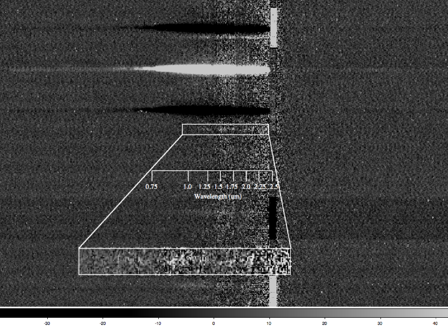
Figure 1: The combined two-dimensional spectrum used as input data. The white rectangle identifies the region of the GRB afterglow spectrum that was used for the analysis. The box height is equal to $4\times fwhm$ corresponding to 21 pixels, ensuring that we completely include both wings of the gaussian. The inset shows a magnification of the same region.

• The real spectrum must be included in the family of models under analysis. This would be relatively difficult, for instance, in the case of quasars or galaxies at moderate resolution, as the intrinsic scatter amongst different types or models is very large. However, GRB afterglows make for an excellent example, as their intrinsic optical spectrum can usually be very well approximated with a single power-law, where the effects of the GRB host gas and dust, the intergalactic medium, and our local extinction, can be superimposed.

• The technical characteristics of the instrument must be well known, in order to model their effect into the simulated data. This includes the total wavelength-dependent efficiency, any possible geometric distortions in the spectral direction, and of course the exact position of the target in the slit image.

• The characteristics of the noise in the CCD must also be modelled accurately, so that the statistical analysis will render an accurate estimate of the model parameters and also of the uncertainties associated to them.

Even though we have not mentioned it explicitly, it is of course necessary to ensure that an accurate first reduction of the data is performed, going from the raw individual images to the combined two-dimensional spectrum, which constitutes the input data for our analysis.

2 Description of the Data

In order to describe our work in detail, we concentrate in the particular case for which we developed our original idea, thus we start by describing those data.

2.1 GRB090423 Afterglow Data

GRB090423 was a gamma-ray burst detected by the Swift satellite on April 23, 2009 (Krimm et al 2009). Early observations in the optical and near infrared distinctly pointed towards the possibility of it being a high-redshift object, when it went undetected for all observers using visible bands, but showed as a relatively bright near-infrared source (Tanvir et al 2009a, Cucchiara et al 2009a). Photometric data alone indicated a very high-redshift nature, with basically zero dust absorption (Cucchiara et al 2009b, Olivares et al 2009). Our group used the Italian 3.6m Telescopio Nazionale Galileo, in the island of La Palma, to obtain a low-resolution spectrum using the Amici prism with the spectrograph NICS (Oliva 2003), and measured its redshift to be $z=8.1^{+0.1}_{-0.3}$ (Thoene et al 2009, Fernandez-Soto et al 2009, Salvaterra et al 2009). A compatible result ($z=8.23^{+0.06}_{-0.07}$) was reached independently by Tanvir et al (2009b, 2009c) using two sets of higher-quality data obtained with the VLT in Chile.

The Amici spectrum covers in a single exposure the wavelength range $0.8-2.5\mu\rm{m}$ with very low resolution ($R\approx 50$) but very high efficiency, and thus became the ideal choice for this kind of analysis. We obtained a total of 128 minutes of on-target exposure time. The exposures were dithered following the usual NIR technique, and combined into a single two-dimensional frame, which is showed in Figure 1. The slit was positioned with the help of a nearby star, whose extracted spectrum will be one of the keys in our analysis.

The position of the star along the slit (measured at the reference position X=600 in the CCD frame) is Y=765. The angular distance between the reference star and the afterglow was $\approx 30$ arcseconds, which corresponds to 120 pixels along the slit. In order to avoid possible issues caused by misalignments or the effect of distortions in the focal plane, we use this distance only as a reference, and perform a careful recentering, as described in the next Section.

3 Description of the Method

Our aim will be to reproduce as perfectly as possible the spectrum of the afterglow of GRB090423, and to reconstruct the spectral equivalent of the wavelength-dependent point spread function as generated when the light passes through the atmosphere, telescope and instrument optics, and reaches the detector. We present in this Section the different steps that we perform to reach this objective.

3.1 Model spectra

We create a library of model spectra, where the basic input parameters are three: the redshift $z$, the slope $\alpha$ in the power-law spectral model $f_{\nu}\propto\lambda^{\alpha}$, and the total neutral Hydrogen column density in the host interstellar medium N(HI), that produces a strong Damped Lyman Alpha (DLA) profile at the host redshift. It is important to include this profile in the analysis, because a dense ($\rm{N(HI)}\gtrsim 10^{21}\rm{cm}^{-2}$) DLA profile would displace the position of the break, thus mimicking a higher redshift. A fourth parameter, the apparent magnitude normalization in the observed $K$ band (at the epoch of our observations) $m_{K}$, will be left as a non-interesting parameter and directly fitted to the data during the process.

Figure 2: Some of the templates used for the analysis. Each column corresponds to a different redshift as labelled in the top panels, and each line to a different spectral slope, as labelled on the leftmost column. Within each panel, the different curves correspond to values of $\log$[N(HI)] varying from 19 to 24 in steps of one.

The effect of the Intergalactic Medium (IGM) at the redshifts of interest ($z\gtrsim 6$) is very simple to include. At such a high redshift the HI absorption is complete—within our observational capabilities—below the Lyman-$\alpha$ line, and as such we include it in the models (Yoshii & Peterson 1994). The putative effects of a significatively different neutral fraction in the IGM were deliberately neglected for two reasons: on one side, the literature on GRB090423 points to a normal environment (i.e. neutral, see Tanvir et al. 2009c); on the other side some authors have shown that those effects are difficult to model and challenging to observe even with better quality data (e.g. Patel et al. 2010).

In other cases one would of course need different parameters. It could be necessary to add dust extinction either at the host or by the Milky Way (or both), with the amount of extinction and even its grain type left as free parameters. We do not consider it here, because the available afterglow photometry indicates a blue object, with an almost complete lack of intrinsic extinction (Fernandez-Soto et al 2009 and Tanvir et al 2009c, in particular their Figure 2 where it is shown how the spectral slope is well represented by a pure power-law). Moreover, given the narrow rest-frame wavelength range that we are observing ($\lambda\approx 1200-2200\AA$), the resolution and signal-to-noise ratio of our data, there is an almost perfect degeneracy between the amount of dust extinction and a change in spectral slope.

Figure 2 shows a selection of spectral templates, sampling part of the parameter space. The full range covered by our templates is $\alpha\in[-1,3]$, $z\in[5,10]$, and N(HI)$\in[10^{20},10^{24}]\rm{cm}^{-2}$. All three ranges safely include the expected values of each variable. All models are normalised to have $AB_{K}=21.3$, a value measured by GROND (Tanvir et al 2009c) at almost exactly the same time our observations were performed. It must be remarked, however, that because of the possibility of slit losses affecting the detected flux, we leave the normalisation factor for the flux as a free parameter, as explained in the next subsection.

Table 1: Stellar data. SDSS and 2MASS photometry were taken from their respective catalogues, and is expressed in their usual reference–AB magnitudes for SDSS, Vega-based for 2MASS.

$$\begin{array}[]{p{0.5\linewidth}l}\hline\cr\vskip 3.0pt plus 1.0pt minus 1.0pt\cr Parameter&Value\\ \vskip 3.0pt plus 1.0pt minus 1.0pt\cr\hline\cr\vskip 3.0pt plus 1.0pt minus 1.0pt\cr SDSS name&J095535.28+180903.8\\ R.A. (J2000)&$09:55:35.286$\\ Dec (J2000)&$+18:09:03.88$\\ Spectral Type&M4V\\ $u_{\rm{SDSS}}$&22.17\pm 0.21\\ $g_{\rm{SDSS}}$&19.27\pm 0.01\\ $r_{\rm{SDSS}}$&17.78\pm 0.01\\ $i_{\rm{SDSS}}$&16.54\pm 0.01\\ $z_{\rm{SDSS}}$&15.91\pm 0.01\\ $J_{\rm{2MASS}}$&14.52\pm 0.03\\ $H_{\rm{2MASS}}$&13.97\pm 0.04\\ $K_{\rm{2MASS}}$&13.77\pm 0.05\\ \vskip 3.0pt plus 1.0pt minus 1.0pt\cr\hline\cr\end{array}$$

3.2 CCD and Instrumental Characteristics

Once satisfied with the set of spectral templates, we need to characterise the observations in terms of spectral resolution, efficiency of the instrument at different wavelengths, noise characterics of the detector, and position of the spectrum along both the spectral and spatial directions.

3.2.1 Instrumental Characteristics

We have used an archival solution to calibrate the Amici spectrum in wavelength. As was described in Fernandez-Soto et al (2009) we needed to add an offset of 5 pixels, determined via comparison with the observed sky absorption features.

As we mentioned in the previous Section, there is a nearby star that falls within the slit—it was in fact used to position the slit, as the afterglow was too dim to be pointed at directly. Its spectral type is M4V, as determined via available SDSS and 2MASS photometry (Adelman-McCarthy et al 2008, Skrutskie et al 2006, see Table 1 for the complete data). We have used the corresponding spectrum from the Bruzual-Persson-Gunn-Stryker library (Bruzual et al 1996) to determine the total efficiency of the instrument as a function of wavelength. In the $0.95-1.1\mu m$ region, corresponding to the Lyman break of a $z\approx 8$ source — the most prominent feature in our GRB spectrum — the spectrum of an M4V star is free from strong spectral features. This, considered together with the low resolution of the spectra and the fact that at higher wavelengths the M4V star shows even less features, allows to rely on the total instrumental efficiency as derived by us.

It must be noted that there is a free factor involved in the calculations, as we cannot ensure that the slit losses in the stellar spectrum are the same in the one corresponding to the afterglow. However, as long as the pointing was reasonably accurate—and we can assume it was from the comparison of the fluxes—at least to first order it will be a single number (i.e., not wavelength-dependent) as the slit angle is obviously the same for both objects.

The seeing at the time of the observations was $\approx 1.4$ arcseconds in the J band, as measured in the acquisition images. The slit width was 1.0 arcsecond, hence we expect some slit losses, and no degradation in resolution induced by the slit width. We show in Figure 3 the measured total efficiency, obtained as the (arbitrarily normalised) ratio of the counts to the model spectrum of the star.

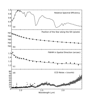
Figure 3: Total efficiency of the atmosphere, telescope, and instrument combination (a). Changes in the spectral position (b) and width (c) with wavelength, and projection of the measured CCD noise (rms counts per pixel) as a function of wavelength (d).

As is usually done when reducing spectroscopic data of very faint sources, we will assume that the shape of the afterglow spectrum in the CCD follows the trace left by the much brighter star (plotted in Figure 3, second panel from the top), which can easily be traced at all wavelengths from 0.8 to 2.5 microns. We determined the distortions along the dispersion axis of the stellar spectrum, fitted it via Legendre polynomials and used it to define the template spectrum position. We determined the vertical offset by using a zero-order solution (an $f_{\nu}$-flat spectrum at $z=8.4$ with HI absorption of $10^{20}$cm^-2) and displacing it vertically, evaluating its likelihood at different positions when compared to the CCD data. We measure an offset of 115.4 pixels (equivalent to 28.8 arcseconds).

The FWHM in the spatial direction of the stellar spectrum varies with wavelength, from $\approx 1.5$ arcseconds at $2.2\mu$m to $\approx 1.2$ arcseconds at $\approx 0.8\mu$m (corresponding to $\approx 5.8$ to $\approx 4.9$ pixels on our plate scale). We have used a smoothed fit to those values (also shown in Figure 3) to reproduce the afterglow spectrum.

3.2.2 CCD Characteristics

The CCD image we are working with is the result of a careful reduction procedure, done following the usual steps for NIR spectroscopy. We have however performed one extra check: we measured the background in detail, to ensure that it is flat in both the spectral and spatial directions, and found no evidence of any trend in any of them, with the background being flat to a fraction of the CCD noise.

We also estimated the CCD noise using different methods. This is a very important step, as we want to determine not only the basic parameters of the GRB afterglow (redshift, spectral slope, and neutral Hydrogen column density), but also to measure confidence limits on both. We decided that the best method consists in using 7 rectangular areas of equal size in the CCD, each one covering the interval $X\in[480,650]$ and 21 pixels in the Y direction. Those boxes were chosen in areas which are free of any (positive or negative) feature. Using them we estimated the noise as a function of X position (that is, wavelength) by using a 3x3 grid around each pixel and all 7 independent images. In this way we obtained a $170\times 21$ mini-CCD noise frame, that we will use for the subsequent chi-square analysis. The projection of this noise array on the Y direction is also shown at the bottom in Figure 3.

We finally computed the noise expected from an ideal $\chi^{2}\equiv 1$ relation when comparing each one of the noise regions to an empty (zero counts) one. The average of the obtained noise values differs from the RMS of our noise array by $\approx 0.3\%$.

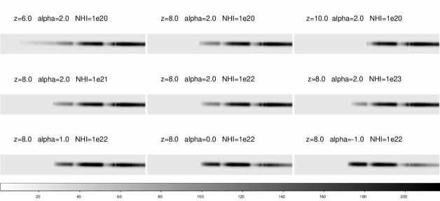
Figure 4: Some of the templates that were shown in Figure 1 are shown here as two-dimensional arrays, after application of the procedures described in Section 3.3.

3.3 Application of the method

We use all the knowledge about the instrument gathered in the previous Subsection to create replicas of the GRB afterglow spectrum, for each one of the templates described in Section 3.1.

In brief, we choose a spectrum template combination (i.e., values of $z$, $\alpha$, and N(HI)) and generate a one-dimensional spectrum using them. We redden this spectrum using the measured Galactic value E($B-V$)=0.03. Then this spectrum is converted to a two-dimensional image, using the measured efficiency, adjusting and block-averaging the wavelength axis to the known dispersion solution of the Amici prism, and convolving it in the spectral direction with a Gaussian function of the measured FWHM at each wavelength. This two-dimensional spectrum is forced to follow the trace that was measured with the stellar spectrum, and is set on a mini-CCD matrix measuring $170\times 21$ pixels, as was described above for the noise image. Figure 4 shows some of the same spectra that were presented in Figure 2, now converted to two-dimensional images with this process.

Each of them is then compared to the real data, using the section of the CCD that contains the GRB afterglow spectrum, centered to the same position of each of the template frames. We do this comparison using a $\chi^{2}$ fit, where the noise array corresponds to the one that was obtained in the previous section. Calling the template $\mathcal{T}(z,\alpha,\rm{N(HI)})$, the CCD data $\mathcal{D}$, and the noise matrix $\mathcal{S}$, and remembering each one of them represents a $170\times 21$ matrix, one obtains:

$$\chi^{2}[z,\alpha,\rm{N(HI)}]=\sum_{i=1}^{170}\sum_{j=1}^{21}\frac{[A\mathcal{T}(z,\alpha,\rm{N(HI)})_{ij}-\mathcal{D}_{ij}]^{2}}{\mathcal{S}_{ij}^{2}},$$ (1)

where $A$ represents a normalization parameter for the flux, which is actually fixed for each template by minimising $\chi^{2}$, which renders

$$A=\frac{\sum_{i=1}^{170}\sum_{j=1}^{21}\mathcal{D}_{ij}\mathcal{T}(z,\alpha,\rm{N(HI)})_{ij}/\mathcal{S}_{ij}^{2}}{\sum_{i=1}^{170}\sum_{j=1}^{21}\mathcal{T}(z,\alpha,\rm{N(HI)})_{ij}^{2}/\mathcal{S}_{ij}^{2}}.$$ (2)

Thus, once the normalisation $A$ is fixed, the calculation of $\chi^{2}$ is straightforward for each template.

4 Results

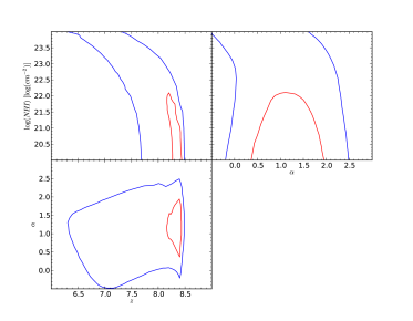
Figure 5: Results of the fitting procedure, projected on each of the two-dimensional planes of parameter space. Red (blue) contours correspond to $1\sigma$ ($2\sigma$) confidence levels.

In Figure 5 we present the result of the calculation above, projected on the different planes of parameter space. Throughout our analysis, we associated the $68.3\%$ and $95.4\%$ confidence levels to $1\sigma$ and $2\sigma$ respectively. As can be seen, the best fit corresponds to $z=8.40$ , $\alpha=1.2$, $\rm{N(HI)}=10^{20.0}\rm{cm}^{-2}$. We have calculated the confidence regions corresponding to the best fit on each of the individual parameters, reaching the results presented in Table 2. We must remark that the best-fit solution represents a value of $\chi^{2}=4019$, which indicates a good fit for our problem, which has $\approx$ 3600 degrees of freedom—albeit obviously most of them void in terms of information content.

As can be observed there is no lower limit to the neutral hydrogen column density. This is a natural observational consequence of the fact that below N(HI)$\approx 2\times 10^{20}$cm^-2 there is no damped profile, and the absorption is not significant at our resolution and signal-to-noise level. On the other end of the column density scale, we stop our analysis at N(HI)$=10^{24}$cm^-2, a value large enough to include even the densest absorbers ever observed. Even larger values could be accomodated, paired to lower redshifts $z<6.5$ and flatter spectral slopes $\alpha<0.5$.

Table 2: Results of the fitting procedure. There is no valid limit to the HI column density at the $2\sigma$ level, which also somehow influences the other parameters (see text for further details).

Parameter	Value	$1\sigma$	$2\sigma$
Redshift	8.40	(8.38,8,45)	(6.67,8.49)
Spectral Slope	1.2	(0.7,1.8)	(0.1,2.2)
$\log$[N(HI)]	20.0	($<20.7$)	—

Figure 6 shows the best-fit spectrum, seen on the two top panels both as a one-dimensional plot and as a clean two-dimensional model, and compared to the real data in the two lower panels.

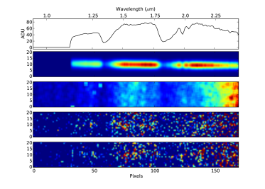
Figure 6: The best-fit spectrum, convolved with the instrument response, is shown in the top panel as a one-dimensional spectrum, and as a clean two-dimensional array in the second one. The third panel shows a $1\sigma$ noise two-dimensional array in the CCD area corresponding to the afterglow spectrum, as described in Section 3.2.2. The fourth panel shows one realization of the CCD noise plus the best-fit spectrum, which can be directly compared to the real data at the bottom panel. The contrast scale is the same in the two latter panels, but not in the previous ones.

We may also use the spectral slope of the GRB afterglow spectrum, as measured from broad-band NIR photometry, as a prior for our analysis. In this way, using the 1-sigma limit presented in Salvaterra et al (2009) for the spectral slope one would obtain a more stringent limit on the redshift, approximately $z>7.5$ at the 2-sigma confidence level.

5 Conclusions

We have presented a different method for the analysis of spectroscopic data, akin in spirit to the one used in X-Ray astronomy and also in photometric resdhift techniques. This method does not attempt to extract a one-dimensional spectrum from the CCD data. On the other hand, we generate simulated two-dimensional spectra from template spectra of known characteristics, and decide which one fits best the real data, choosing the best-fit parameters as the solutions to the problem.

We have used this method to perform a careful analysis of a very low signal-to-noise spectrum of the afterglow of the very distant GRB090423, showing that it is possible to extract information from this kind of data, further than is usually assumed. Our best result ($z=8.40^{+0.05}_{-0.02}$) is slightly higher than previous results obtained using the same data (Salvaterra et al 2009) or data from other sources (Tanvir et al 2009c), although still compatible well within the $2\sigma$ confidence level. We believe our confidence intervals to be reliable, given the full analysis of the noise characteristics performed in this work.

The same method can be applied to other cases where the source belongs to a well-defined spectral class of objects, and there is a need to extract the maximum possible information from low-quality data. This is usually the case for faint, rapidly fading GRB afterglows, and we expect this method to be used in future measurements.