Ground states of trapped spin-1 condensates in magnetic field

Abstract

We consider a spin-1 Bose-Einstein condensate trapped in a harmonic potential under the influence of a homogeneous magnetic field. We investigate spatial and spin structure of the mean-field ground states under constraints on the number of atoms and the total magnetization. We show that the trapping potential can make the antiferromagnetic condensate separate into three, and ferromagnetic condensate into two distinct phases. In the ferromagnetic case, the magnetization is located in the center of the harmonic trap, while in the antiferromagnetic case magnetized phases appear in the outer regions. We describe how the transition from the Thomas-Fermi regime to the single-mode approximation regime with decreasing number of atoms results in the disappearance of the domains. We suggest that the ground states can be created in experiment by adiabatically changing the magnetic field strength.

I Introduction

Bose-Einstein condensates with spin degrees of freedom Ho attracted in recent years great interest due to the unique possibility of exploring fundamental concepts of quantum mechanics in a remarkably controllable and tunable environment. The ability to generate spin squeezing and entanglement Entanglement makes spinor Bose gases promising candidates for applications as quantum simulators QS , in quantum information QI , and for precise measurements Measurement . Moreover, spinor condensates were successfully used to recreate many of the phenomena of condensed matter physics in experiments displaying an unprecedented level of control over the quantum system. In particular, spin domains Stenger_Nat_1998 ; Ketterle_Metastable ; Sadler_Nat_2006 , spin mixing Mixing ; Chang_PRL_2004 , and spin vortices Ketterle_Coreless were predicted and observed.

The ground states of spin-1 condensates in homogeneous magnetic field have been studied in a number of previous works Zhang_NJP_2003 ; Stenger_Nat_1998 ; Ueda_SBS ; SMA ; Zhou ; Matuszewski_PS . The typical procedure consists of minimization of the total energy under constraints on the number of atoms and the longitudinal magnetization, which is well conserved in typical experimental conditions Chang_PRL_2004 . Most of the studies, however, considered the condensate in the single-mode approximation, which assumes that the spin components share the same spatial profile SMA ; Zhang_PRA_2005 , ignoring the possibility of phase separation.

In Ref. Zhang_NJP_2003 , the breakdown of the single-mode approximation was shown numerically for a condensate confined in a harmonic potential. In a recent paper Matuszewski_PS , we studied the possibility of phase separation in the case of an untrapped condensate, and demonstrated that this phenomenon can take place in an antiferromagnetic condensate, leading to the splitting into two distinct phases. On the other hand, ferromagnetic condensates were found not to display phase separation for any values of parameters. However, the trapping potential, present in any experimental realization, can strongly influence the structure of the ground states. Indeed, in the context of binary condensates, it was previously shown that spatial separation of components can be induced by an external potential Timmermans . This phenomenon was called “potential separation” as opposed to “phase separation” which occurs spontaneously also in the untrapped case. Moreover, the external potential determines the spatial structure of phase separated states. In general, phases that are characterized by energetically unfavorable interatomic interactions are moved towards the outer, low density regions, as demonstrated in spin-imbalanced Fermi systems Hulet_ImbalancedFermions and spinful bosons Cornell_BinarySeparation ; Matuszewski_PS .

In this paper, we investigate in detail the spatial separation of spin phases in the ground states of spin-1 condensates trapped in harmonic potentials. We find that the phase diagram of a trapped condensate is substantially different from the one of an untrapped condensate. We show that the external potential can make the antiferromagnetic condensate separate into three, and ferromagnetic condensate into two distinct phases. Furthermore, we suggest an experimental method for the creation of these ground states by adiabatically changing the magnetic field strength.

The paper is organized as follows. Section II reviews the mean-field model of a spin-1 condensate in a homogeneous magnetic field and the possible spin phases. Section IV presents analytical and qualitative results describing the structure of ground states in the Thomas-Fermi approximation. In Section V we treat the problem numerically in a systematic way and demonstrate the crossover between the Thomas-Fermi and single-mode-approximation regimes. Section VI describes an experimental method of creation of the ground states. Section VII concludes the paper.

II Model

We consider a dilute spin-1 BEC in a homogeneous magnetic field pointing along the $z$ axis. We start with the mean-field Hamiltonian $H=H_{\rm S}+H_{\rm A}$,

$$H=\sum_{j=-,0,+}\int d\mathbf{r}\,\psi_{j}^{*}\left(-\frac{\hbar^{2}}{2m}\nabla^{2}+\frac{c_{0}}{2}n+V({\bf r})\right)\psi_{j}+H_{A},$$ (1)

where $\psi_{-},\psi_{0},\psi_{+}$ are the wavefunctions of atoms in magnetic sublevels $m_{\rm f}=-1,0,+1$, $M$ is the atomic mass, $V({\bf r})$ is an external potential and $n=\sum n_{j}=\sum|\psi_{j}|^{2}$ is the total atom density. The asymmetric (spin dependent) part of the Hamiltonian is given by

$$H_{\rm A}=\int d\mathbf{r}\left(\sum_{j=-,0,+}E_{j}n_{j}+\frac{c_{2}}{2}|{\bf F}|^{2}\right)$$ (2)

where $E_{j}$ is the Zeeman energy shift for state $\psi_{j}$ and the spin density is,

$${\bf F}=(F_{x},F_{y},F_{z})=(\psi^{\dagger}\hat{F}_{x}\psi,\psi^{\dagger}\hat{F}_{y}\psi,\psi^{\dagger}\hat{F}_{z}\psi)$$ (3)

where $\hat{F}_{x,y,z}$ are the spin-1 matrices Isoshima_PRA_1999 and $\psi=(\psi_{+},\psi_{0},\psi_{-})$. The spin-independent and spin-dependent interaction coefficients are given by $c_{0}=4\pi\hbar^{2}(2a_{2}+a_{0})/3m$ and $c_{2}=4\pi\hbar^{2}(a_{2}-a_{0})/3m$, where $a_{S}$ is the s-wave scattering length for colliding atoms with total spin $S$. The total number of atoms and the total magnetization in the direction of the magnetic field

$$N =\int nd\mathbf{r}\,,$$ (4)

$$\mathcal{M} =\int F_{z}d\mathbf{r}=\int\left(n_{+}-n_{-}\right)d\mathbf{r}\,,$$ (5)

are conserved quantities. The Zeeman energy shift for each of the components, $E_{j}$ can be calculated using the Breit-Rabi formula Wuster

$$E_{\pm} =-\frac{1}{8}E_{\rm HFS}\left(1+4\sqrt{1\pm\alpha+\alpha^{2}}\right)\mp g_{I}\mu_{B}B\,,$$

$$E_{0} =-\frac{1}{8}E_{\rm HFS}\left(1+4\sqrt{1+\alpha^{2}}\right)\,,$$ (6)

where $E_{\rm HFS}$ is the hyperfine energy splitting at zero magnetic field, $\alpha=(g_{I}+g_{J})\mu_{B}B/E_{\rm HFS}$, where $\mu_{B}$ is the Bohr magneton, $g_{I}$ and $g_{J}$ are the gyromagnetic ratios of nucleus and electron, and $B$ is the magnetic field strength. The linear part of the Zeeman effect gives rise to an overall shift of the energy, and so we can remove it with the transformation

$$H\rightarrow H+(N+\mathcal{M})E_{+}/2+(N-\mathcal{M})E_{-}/2\,.$$ (7)

This transformation is equivalent to the removal of the Larmor precession of the spin vector around the $z$ axis Matuszewski_PRA_2008 ; Ueda_SBS . We thus consider only the effects of the quadratic Zeeman shift. For sufficiently weak magnetic field we can approximate it by $\delta E=(E_{+}+E_{-}-2E_{0})/2\approx\alpha^{2}E_{\rm HFS}/16$, which is always positive.

The asymmetric part of the Hamiltonian (2) can now be rewritten as

$$H_{\rm A}=\int d\mathbf{r}\,\left(-\delta E\,n_{0}+\frac{c_{2}}{2}|{\bf F}|^{2}\right)=\int d\mathbf{r}\,n\,e(\mathbf{r})\,,$$ (8)

where the energy per atom $e(\mathbf{r})$ is given by Zhang_PRA_2005

$$e= -\delta E\rho_{0}+\frac{c_{2}n}{2}|\mathbf{f}|^{2}=-\delta E\rho_{0}+\frac{c_{2}n}{2}\left(|{\bf f}_{\perp}|^{2}+m^{2}\right)\,,$$

$$|{\bf f}_{\perp}|^{2}= 2\rho_{0}(1-\rho_{0})+2\rho_{0}\sqrt{(1-\rho_{0})^{2}-m^{2}}\cos(\theta)\,.$$ (9)

We express the wavefunctions as $\psi_{j}=\sqrt{n\rho_{j}}\exp(i\theta_{j})$ where the relative densities are $\rho_{j}=n_{j}/n$. We also introduced the relative phase $\theta=\theta_{+}+\theta_{-}-2\theta_{0}$, spin per atom $\mathbf{f}=\mathbf{F}/n$, and magnetization per atom $m=f_{z}=\rho_{+}-\rho_{-}$. The perpendicular spin component per atom is $|{\bf f}_{\perp}|^{2}=f_{x}^{2}+f_{y}^{2}$.

The Hamiltonian (1) gives rise to the Gross-Pitaevskii equations describing the mean-field dynamics of the system

$$i\hbar\frac{\partial\psi_{\pm}}{\partial t} =\left[\mathcal{L}+c_{2}(n_{\pm}+n_{0}-n_{\mp})\right]\psi_{\pm}+c_{2}\psi_{0}^{2}\psi_{\mp}^{*}\,,$$ (10)

$$i\hbar\frac{\partial\psi_{0}}{\partial t} =\left[\mathcal{L}-\delta E+c_{2}(n_{+}+n_{-})\right]\psi_{0}+2c_{2}\psi_{+}\psi_{-}\psi_{0}^{*}\,,$$

where $\mathcal{L}$ is given by $\mathcal{L}=-\hbar^{2}\nabla^{2}/2M+c_{0}n+V({\bf r})$.

By comparing the kinetic energy with the interaction energy, we can determine the healing length $\xi=2\pi\hbar/\sqrt{2Mc_{0}n}$ and the spin healing length $\xi_{s}=2\pi\hbar/\sqrt{2Mc_{2}n}$. These quantities give the length scales of spatial variations in the condensate profile induced by the spin-independent or spin-dependent interactions, respectively. Analogously, we define the magnetic healing length as $\xi_{B}=2\pi\hbar/\sqrt{2M\delta E}$.

In spin-1 condensates created to date, the $a_{0}$ and $a_{2}$ scattering lengths have similar magnitudes. The spin-dependent interaction coefficient $c_{2}$ is then much smaller than its spin-independent counterpart $c_{0}$. For example, this ratio is about 1:30 in a ²³Na condensate and 1:220 in a ⁸⁷Rb condensate far from Feshbach resonances Beata . Consequently, changing the total density $n$ requires much more energy than changing the relative populations of spin states $n_{j}$. In our considerations we will treat the total atom density profile $n(\mathbf{r})$ as a constant, close to the Thomas-Fermi profile for a given potential $V(\mathbf{r})$.

III Homogeneous stationary states

We recall the possible phases of spin-1 condensates in magnetic field Matuszewski_PS . The stationary solutions in the case of a vanishing potential, $V({\bf r})=0$, have the form

$$\psi_{j}(\mathbf{r},t)=\sqrt{n_{j}}{\rm e}^{-i(\mu_{j}+\mu_{S})t+i\theta_{j}}\,,$$ (11)

where $\mu_{S}=c_{0}n/\hbar$ is a constant. These solutions are stationary in the sense that the number of atoms in each magnetic sublevel $n_{j}$ is constant in time, but the relative phases may change as a result of an additional spin precession around $z$, as long as the phase matching condition

$$\mu_{+}+\mu_{-}=2\mu_{0}\,,$$ (12)

is fulfilled Isoshima_PM ; Matuszewski_PRA_2008 . Because the symmetric part of the Hamiltonian in (1) is constant, the relevant part of the Hamiltonian is given by Eq. (8).

The Hamiltonian (1) and GP equations (10) are invariant under the gauge transformation $\psi_{j}\rightarrow\psi_{j}\exp(-i\beta)$ and rotation around the $z$ axis $\psi_{j}\rightarrow\psi_{j}\exp(-iF_{z}\gamma)$, which transform the wavefunction components according to

$$\left(\begin{array}[]{c}\psi_{+}\\ \psi_{0}\\ \psi_{-}\end{array}\right)\rightarrow{\rm e}^{-i\beta}\left(\begin{array}[]{c}{\rm e}^{-i\gamma}\psi_{+}\\ \psi_{0}\\ {\rm e}^{i\gamma}\psi_{-}\end{array}\right)\,.$$ (13)

Hence the solutions can be classified using the relative densities $\rho_{j}=n_{j}/n$ and a single relative phase $\theta=\theta_{+}+\theta_{-}-2\theta_{0}$, with the chemical potentials $\mu_{j}$ given as solutions to Eqs. (10). We note that for stationary solutions with all three components populated the relative phase must take one of two values, $\theta=0$ or $\theta=\pi$. We call the former “phase-matched” states (PM) and the latter “anti-phase-matched” (APM) states. The names derive from the fact that within the continuum of states satisfying the spin rotations (13) there is a set $(\psi_{+},\psi_{0},\psi_{-})$ with all components in phase for the PM states, and a set with $\psi_{+}$ and $\psi_{0}$ in phase but with $\psi_{-}$ $\pi$ out of phase for the APM states.

In general, the possible stationary states can be classified as follows

1. Nematic state ($\rho_{0}$), with all the atoms in the $m_{f}=0$ component, $\psi=(0,\psi_{0},0)$. The chemical potential, spin density and energy per atom are equal to

   $$\hbar\mu_{0}=-\delta E,\quad|{\bf f}|=0,\quad e=-\delta E\,.$$ (14)

2. Magnetized states ($\rho_{-}$ and $\rho_{+}$), with all the atoms in the $m_{f}=-1$ or in the $m_{f}=+1$ component, $\psi=(0,0,\psi_{+})$ or $\psi=(\psi_{-},0,0)$

   $$\hbar\mu_{\pm}=c_{2}n,\quad|m|=1,\quad|{\bf f}_{\perp}|=0,\quad e=\frac{c}{2}\,.$$ (15)

3. Two-component or stretched states (2C), with $\psi=(\psi_{-},0,\psi_{+})$ and arbitrary magnetization

   $$\hbar\mu_{\pm}=\pm c_{2}nm,\quad|{\bf f}_{\perp}|=0,\quad e=\frac{c}{2}m^{2}\,.$$ (16)

4. Phase-matched states (PM), where all three sublevels are populated, $\psi=(\psi_{-},\psi_{0},\psi_{+})$, and the relative phase is equal to $\theta=0$.

5. Anti-phase-matched states (APM), similar as the PM state but with $\theta=\pi$.

The parameters of the PM and APM phases cannot be expressed by analytical formulas in the general case. Since all three components are populated in these states, the magnetization perpendicular to the magnetic field direction, $|{\bf F}_{\perp}|=\sqrt{2}|\psi_{+}\psi_{0}^{*}+\psi_{0}\psi_{-}^{*}|$, is nonzero. Hence the axial symmetry of the system is broken Ueda_SBS .

These above classification is also applicable to inhomogeneous condensates within the single-mode approximation (SMA), which assumes that the spin components share the same spatial profile SMA ; Zhang_PRA_2005 , after replacing $n$ with $\langle n\rangle$. This assumption is true eg. when the condensate size is much smaller than the spin healing length $\xi_{s}$ and the magnetic healing length $\xi_{B}$.

IV Ground states in the Thomas-Fermi approximation

In this section, we investigate the structure of the ground states in harmonic potential within the Thomas-Fermi (TF) approximation (or local density approximation), neglecting the kinetic energy in the Hamiltonian (1). This approximation is justified when the spatial variation of the condensate wavefunction gives a contribution that is relatively small, in particular when the size of the condensate is much larger than both $\xi_{s}$ and $\xi_{B}$.

Within our assumptions, the asymmetric part of the energy (2) is a small contribution to the total energy. The profile of the total density is determined by the minimization of the symmetric part of the free energy with a fixed particle number

$$K_{\rm S}=\int\left(\frac{c_{0}}{2}n+V\right)n\,d\mathbf{r}-\mu N\,,$$ (17)

where $\mu$ is the Lagrange multiplier corresponding to the chemical potential. The minimization of this functional gives the well known Thomas-Fermi profile $c_{0}n(\mathbf{r})+V(\mathbf{r})=\mu={\rm const}$.

Analogously, to determine the spin structure, we minimize the asymmetric part of the energy $E_{\rm A}$ with a fixed total magnetization $M$

$$K_{\rm A}=\int e(n,m)n\,d\mathbf{r}-pM,\,\,M=\int mn\,d\mathbf{r}.$$ (18)

The minimum of this functional requires that

$$\frac{\partial e(n,m)}{\partial m}=p=\mathrm{const},$$ (19)

when moving from one point in space to another. This condition is not applicable to the completely magnetized $\rho_{+}$, $\rho_{-}$ and the unmagnetized $\rho_{0}$ phase, for which $\partial e/\partial m$ is undefined Matuszewski_PS .

IV.1 Antiferromagnetic case ($c_{2}>0$)

Since we work within the Thomas-Fermi approximation and neglect the spatial derivatives, at each point in space the local phase corresponds to a ground state of a homogeneous condensate Matuszewski_PS . Nevertheless, the change of local parameters (density and magnetization) in space may lead to the change of the local ground state and the appearance of spatial domains.

In the case of an antiferromagnetic condensate, there are five possible local ground state phases: $\rho_{+}$, $\rho_{-}$, $\rho_{0}$, 2C and APM Matuszewski_PS . The last two of them allow for a variation of the local magnetization. In the case of the 2C phase, the condition (19) gives

$$\frac{\partial e}{\partial m}=nm=n_{+}-n_{-}=\mathrm{const},$$ (20)

hence the difference in the density of atoms in the $m=+1$ and the $m=-1$ components is constant. For the APM state, the asymmetric energy (further on we call it simply the energy) is not an analytical function of $n$ and $m$, and we approximate it with the formula $e_{\rm APM}\approx(|m|-1)\delta E+|m|c_{2}n/2$, which gives less than $10\%$ error for any $n$ and $m$. The condition (19) gives

$$\frac{\partial e}{\partial m}=\delta E+\frac{c_{2}n}{2}=\mathrm{const},$$ (21)

which obviously cannot be fulfilled if the density profile is not homogeneous. Consequently, the APM phase is unstable, because the transfer of magnetization from the central, high density area to the outer regions is always energetically favorable. Hence, the ground state can contain $\rho_{+}$, $\rho_{-}$, $\rho_{0}$, and/or 2C domains, the latter fulfilling the condition (20).

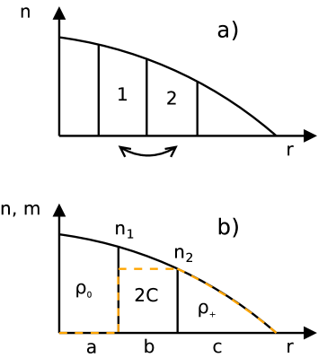
Figure 1: Schematic profiles of phase separated states. (a) The swapping of two domains can change the total energy, even if the number of atoms in each of them is kept constant. (b) The structure of the ground state of an antiferromagnetic condensate composed of three phases. The dashed line shows the local magnetization.

The other question is the placement of the domains. Since the local ground state depends on the density, the domains arrange according to the distance from the center of the trap, as in Fig. 1(a). Let us consider two domains, one of them composed of phase X placed at the area 1 and the other composed of phase Y placed at the area 2, containing equal number of atoms. If the energy per atom of the phase X is constant, (which is the case for the $\rho_{0}$ phase), then swapping of the domains as in Fig. 1(a) will not lead to the change of its energy

$$\Delta E_{X}=e_{\rm X}\left(\int_{1}n\,d\mathbf{r}-\int_{2}n\,d\mathbf{r}\right)=0\,.$$ (22)

On the other hand, if the energy per atom of the phase Y is proportional to the number of atoms, $e_{\rm Y}=an$, as for the $\rho_{\pm}$ or 2C phases, the difference in its energy is

$$\Delta E_{Y}=a\left(\int_{1}n^{2}\,d\mathbf{r}-\int_{2}n^{2}\,d\mathbf{r}\right)=aB,\,\mathrm{where}\,B>0\,.$$ (23)

In result, it is energetically favorable for the $\rho_{0}$ phase to stay in the high density area in the center of the trap. Moreover, the $\rho_{+}$ or $\rho_{-}$ phase will be moved further than the 2C phase to the outer areas, since their coefficient $a$ is larger.

We obtain the general domain structure depicted in Fig. 1(b), shown for positive $M$ (for negative $M$, the local magnetization is opposite and the $\rho_{+}$ state is replaced by $\rho_{-}$). The boundary between the phases $\rho_{0}$ and 2C corresponds to a first order phase transition, and the boundary between the phases 2C and $\rho_{+}$ to a second order phase transition Matuszewski_PS . We note that not all of the phases must be present. If all three domains are present, we can derive the relation between $n_{1}$ and $n_{2}$ by calculating the change of the total energy when changing the domain sizes $a$, $b$ and $c$. Since the magnetization is conserved, we have $\Delta M=b\Delta n_{2}-n_{2}\Delta a=0$ and consequently $\Delta n_{2}/n_{2}=\Delta a/b$. The change of energy is

$$\Delta E_{\rm A} =\left(-\delta En_{1}-\frac{c_{2}}{2}n_{2}^{2}\right)\Delta a+\frac{c_{2}}{2}\Delta\!\left(n_{2}^{2}\right)=$$

$$=\left(-\delta En_{1}+\frac{c_{2}}{2}n_{2}^{2}\right)\Delta a.$$ (24)

This gives the equilibrium condition $\delta En_{1}=c_{2}n_{2}^{2}/2$, and consequently the necessary (but not sufficient) requirement

$$\delta E<\frac{c_{2}}{2}n_{\rm max}$$ (25)

for the coexistence of all three phases, where $n_{\rm max}$ is the maximum density in the center of the trap.

IV.2 Ferromagnetic case ($c_{2}<0$)

In the case of a ferromagnetic condensate, the possible ground state phases are $\rho_{+}$, $\rho_{-}$, $\rho_{0}$, and PM Matuszewski_PS . Since it is difficult to propose a simple analytical formula for the energy of the PM phase, we resort to a qualitative analysis using the condition (19).

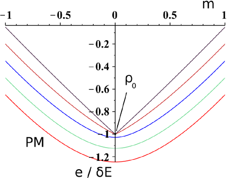
Figure 2: Normalized energy per atom versus magnetization for the possible ground states of the ferromagnetic condensate. The lines correspond to normalized densities (from top to bottom) $|c_{2}|n/\delta E=0.1,0.4,0.7,1.0,1.3$. All the paths fulfilling the condition $de/dm=\mathrm{const}$, with the exception of completely magnetized states, arrive at the central point corresponding to the $\rho_{0}$ state in the low $n$ limit.

In Fig. 2 we show the normalized energy per atom $e/\delta E$ of these states in function of the local magnetization $m$ for several values of the normalized density $c_{2}n/\delta E$. The central point corresponds to the $\rho_{0}$ phase, while the $\rho_{+}$ and $\rho_{-}$ phases correspond to the limits $m=\pm 1$. The possible Thomas-Fermi profiles correspond to sets of points in the $e,m$ plane that fulfill the condition $\partial e/\partial m={\rm const}$. At constant $\delta E$, the magnitude of this derivative generally increases with decreasing $n$ (when moving from the center of the trap to the less populated regions), which can be seen from the gradually “steeper” shape of the top curves. To keep $\partial e/\partial m$ constant, the magnitude of magnetization has to decrease, and eventually we arrive at the point $\rho_{0}$ at a low enough $n$. In this way, we obtain a phase separated state consisting of PM and $\rho_{0}$ domains. The only exceptions from this are the purely $\rho_{0}$ state for $M=0$ and high enough $\delta E$, and purely $\rho_{+}$ and $\rho_{-}$ states for $M=\pm 1$.

The placement of domains in the PM+$\rho_{0}$ state can be deduced in a similar way as in the antiferromagnetic case. The energy per atom in the $\rho_{0}$ phase is constant, while the energy in the PM phase is a decreasing function of density, due to the spin-dependent atomic interaction with a negative $c_{2}$. Hence the atoms in the PM state will reside in the trap center, where the energy is the highest.

V Numerical results

V.1 Potential induced spatial separation

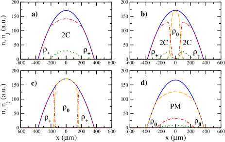
Figure 3: Examples of ground states of an antiferromagnetic (a-c) and a ferromagnetic (d) condensate in the quasi-1D case. (a) $\mathrm{2C}+\rho_{+}$ state for $m=0.8$ and $\delta E/c_{2}n_{\rm max}=0.05$, (b) $\rho_{0}+\mathrm{2C}+\rho_{+}$ state for $m=0.6$ and $\delta E/c_{2}n_{\rm max}=0.17$, (c) $\rho_{0}+\rho_{+}$ state for $m=0.4$ and $\delta E/c_{2}n_{\rm max}=0.37$, and (d) $\mathrm{PM}+\rho_{0}$ state for $m=0.1$ and $\delta E/c_{2}n_{\rm max}=-1.13$. The $n_{+}$, $n_{0}$, and $n_{-}$ components are depicted by dash-dotted, dashed, and dotted lines, respectively, and the solid lines show the total density. Here $\omega_{\perp}=2\pi\times 10^{3}\,$Hz, other parameters are $N=8.4\times 10^{3}$ ²³Na atoms, $\omega_{z}=2\pi\times 2.5\,$Hz in (a-c) and $N=8.4\times 10^{3}$ ⁸⁷Rb atoms, $\omega_{z}=2\pi\times 1.7\,$Hz in (d).

In this section we present examples of numerically determined ground state profiles for both antiferromagnetic and ferromagnetic condensates in quasi 1D and quasi 2D setups. The ground state profiles for a quasi-1D condensate were found numerically by solving the 1D version of Eqs. (10) Matuszewski_PS with rescaled interaction coefficients $c_{0}^{\rm 1D},c_{2}^{\rm 1D}=(m\omega_{\perp})/(2\pi\hbar)c_{0},c_{2}$, where $\omega_{\perp}$ is the transverse trapping frequency. The Fermi radius of the transverse trapping potential is smaller than the spin healing length, and the nonlinear energy scale is much smaller than the transverse trap energy scale, which allows us to reduce the problem to one spatial dimension Beata ; NPSE . The solutions were found numerically using the normalized gradient flow method BaoLim , which is able to find a state that minimizes the total energy $E$ for given $N$ and $M$, and fulfills the phase matching condition (12). The conventional imaginary time method is not suitable for this problem since the normalization of the wavefunction effectively imposes that the chemical potentials $\mu_{j}$ are equal, thus failing to take into account some of the ground states. We note that the direction of the magnetic field with respect to the trap orientation does not influence our results, since only the contact interactions are taken into account in our model.

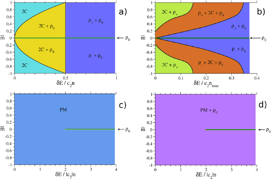
Figure 4: Diagrams of phase separation of an antiferromagnetic (a,b) and a ferromagnetic (c,d) condensate in the quasi-1D case. The left column corresponds to the untrapped case (spontaneous phase separation), while the right column corresponds to a condensate in a harmonic potential.

The setup consists of a highly elongated cigar-shaped harmonic trap, the longitudinal size of the condensate being much larger than other length scales, i.e. the spin and magnetic healing lengths $\xi_{s}$ and $\xi_{B}$. This ensures that the contribution of the kinetic energy (e.g. at the boundaries between domains) is small compared to other energy scales in the system, which is the requirement for the application of the Thomas-Fermi approximation. Figs. 3(a)-(c) show typical ground state profiles of an antiferromagnetic condensate in various regimes of parameters. In accordance with the theoretical considerations, the domain structure, in general, consists of spatially separated $\rho_{0}$, 2C, and $\rho_{+}$ phases, and the arrangement of domains is such that the more magnetized the phase, the farther it is from the trap center. In the 2C phase, the difference between the density of $m=+1$ and $m=-1$ atoms is constant, in agreement with the condition (20).

As a rule, the 2C+$\rho_{+}$ state (a) is the ground state at low magnetic fields, the three-phase state (b) occurs in the transitory regime, and the $\rho_{0}$+$\rho_{+}$ state (c) appears at stronger magnetic fields. This can be understood by noting that the Zeeman energy of the $m=0$ component is decreased with respect to the $m=\pm 1$ components when increasing the magnetic field strength. This is the reason for the appearance of the $\rho_{0}$ domain which eventually replaces the 2C phase completely, in accordance with the condition (25). Another possibility is the unmagnetized condensate ($M=0$), where the whole condensate consists of a single $\rho_{0}$ domain (not shown).

In the case of a ferromagnetic condensate, the ground state generally consists of PM and $\rho_{0}$ domains, as depicted in Fig. 3(d). The magnetized PM phase is placed at the center, again in agreement with the results of Sec. IV. At low magnetic fields the $\rho_{0}$ domains can become very small and eventually disappear when their size becomes smaller than the spin healing length. In this case, the condensate is completely composed of the PM phase. In a unmagnetized condensate ($M=0$), the phase separated PM+$\rho_{0}$ state is preferred at low magnetic fields, $\delta E<2|c_{2}|n$ Matuszewski_PS , otherwise a single $\rho_{0}$ domain is present.

In Fig. 4, we summarize the above results in a systematic way and juxtapose them with the ones obtained in the case of an untrapped condensate Matuszewski_PS . It is clear that the phase separation has a qualitatively different character in the presence of the trapping potential. Although there are similarities, in general the ground states have a different structure. In particular, the antiferromagnetic condensate can separate into three distinct phases in the presence of the trapping potential, while the maximum number of phases is two in the untrapped phase. In the case of a ferromagnetic condensate, the potential induces separation into two phases, while the untrapped condensate is always homogeneous.

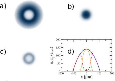
Figure 5: The $\rho_{0}+\rho_{+}$ state in a quasi-2D harmonic trap. The densities of the (a) $m=+1$, (b) $m=0$ and (c) $m=-1$ components are shown, together with the cross section of the densities along the $x$ axis (d). The parameters are $N=2.5\times 10^{6}$ ²³Na atoms, $m=0.8$, $B=0.15\,$G, $\delta E/c_{2}n_{\rm max}=0.15$, $\omega_{xy}=2\pi\times 10\,$Hz, $\omega_{z}=2\pi\times 10^{3}\,$Hz.

In Fig. 5 we present an example of a phase separated $\rho_{0}$+$\rho_{+}$ ground state of an antiferromagnetic condensate in the two dimensional geometry. The domains arrange radially, with the unmagnetized phase in the center, in agreement with the results of Sec. IV. Atoms of the $m=-1$ component are present only at the boundary between the two domains. We note that in the 2D geometry it would be difficult to obtain a clear three phase state, due to the limited number of atoms available in experiment.

V.2 Crossover between the Thomas-Fermi and the single-mode regime

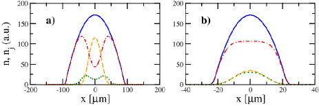
Figure 6: Crossover from the Thomas-Fermi regime to the single mode regime and the disappearance of spin domains. The parameters are the same as in Fig. 3(b), except that the number of atoms was decreased (a) $4\times$ and (b) $16\times$, while the trap frequency was increased to keep the density constant. Here the spin healing length is $\xi_{s}=17\mu$m and the magnetic healing length is $\xi_{B}=42\mu$m.

The above results, corresponding to the Thomas-Fermi (TF) regime, are characteristic for the case when the size of the condensate is much larger than the spin healing length $\xi_{s}$ and the magnetic healing length $\xi_{B}$. On the other hand, in the opposite limit of a small condensate, the ground state structure is well described by the single mode approximation (SMA) SMA , where all three magnetic components share the same spatial profile. However, typical experimental conditions may correspond to an intermediate regime, where condensate size is comparable to $\xi_{s}$ or $\xi_{B}$. An example of the crossover between TF and SMA regimes is presented in Fig. 6. The parameters correspond to the three-phase state from Fig. 3(b), but the number of atoms was decreased $4\times$ and $16\times$ in (a) and (b), while the trap frequency was increased to keep the density constant. The domain structure transforms gradually towards a single-mode ground state. The thickness of the boundaries between domains is determined by the energy difference between neighboring phases. In particular, the boundary between 2C and $\rho_{+}$ domains is of the order of $\xi_{s}$, while the boundary between $\rho_{0}$ and 2C domains is significantly larger, of the order of $\xi_{B}$. This is clearly visible in Fig. 6(b), where the size of the condensate is about two times larger than $\xi_{s}$ but already smaller than $\xi_{B}$. in this case, small $\rho_{+}$ domains can still be distinguished, but 2C and $\rho_{0}$ domains merged into a single APM phase domain, which is the ground state in the SMA limit Matuszewski_PS ; Zhang_NJP_2003 .

VI Generation of spin domains

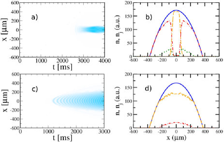
Figure 7: Generation of the ground state profiles by adiabatically changing the magnetic field. The magnetic field is gradually increased from zero to the final value $B=0.15\,$G during $t=4\,$s for sodium condensate (a,b), and decreased from $B=0.5\,$G to $B=0.35\,$G during $t=3\,$s (c,d) for rubidium. The frames (a) and (c) show the time dependence of the atom density in the $m=0$ and $m=+1$ component, respectively, and the right column shows the final domain profiles. The parameters are as in Fig. 3, except $m=0.6$ in (a,b) and $m=0$ in (c,d).

From the practical point of view, it is important to propose a reliable method for the generation of the above ground states in experiment. We show that the method of adiabatic change of the magnetic field, introduced in Matuszewski_FNT , can be used for this purpose. In the case of an antiferromagnetic condensate, we start from the initial ground state where all the atoms are in the $m=-1$ sublevel. Next, part of the atoms is transferred to the $m=+1$ sublevel Transfer , and the magnetic field is switched off. In this way, we obtain a system close to the zero-field ground state with an arbitrary magnetization, determined by the amount of atoms transferred. Next, we gradually increase the magnetic field strength in an adiabatic process according to the formula

$$B=\sqrt{\frac{t}{t_{\rm switch}}}\;B_{\rm final}$$ (26)

where $t=0$ at the beginning of the switching process, $t_{\rm switch}$ is the switching time, and $B_{\rm final}$ is the desired final value of the magnetic field. The form of Eq. (26) assures that the quadratic Zeeman splitting grows linearly in time. In Figs. 7(a,b) we present an example of the generation process simulated by numerical solution of the Gross-Pitaevskii equations (10). Fig. 7(a) shows the time dependence of the atom density in the initially unoccupied $m=0$ component, and Fig. 7(b) shows the final domain profile. This should be compared with the ground state profile in Fig. 3(b), which corresponds to the same parameter values.

In the case of a ferromagnetic condensate, the above scenario has to be slightly modified. We begin with strong magnetic field, in the regime where the quadratic Zeeman energy dominates. The initial state consists of atoms in the $m=0$ sublevel only, which is the ground state in these conditions, see Fig. 4(d). Here, we are limited to the states with the total magnetization $M=0$ only. The magnetic field is then decreased, and after crossing the point of phase transition additional PM domains appear. This scenario and the example of the final state are demonstrated in Figs. 7(c,d). Since $M=0$, the curves corresponding to densities of $m=-1$ and $m=1$ atoms are overlapping. The PM domain is located in the center of the trap, where all three components are nonzero.

VII Conclusions

We investigated spin-1 Bose-Einstein condensates trapped in a harmonic potentials under the influence of a homogeneous magnetic field. We demonstrated that the trapping potential has a strong influence on the structure of ground states in these systems, and can make the antiferromagnetic condensate separate into three, and ferromagnetic condensate into two distinct phases. We studied the crossover from the Thomas-Fermi regime to the single mode approximation regime, where the condensate size becomes smaller than the spin healing length and the spatial structure of ground states disappears. We suggested an experimental method for creation of these states by adiabatically changing the magnetic field strength.

- (1) T.-L. Ho, Phys. Rev. Lett. 81, 742 (1998); T. Ohmi and K. Machida, J. Phys. Soc. Jpn. 67, 1822 (1998).
- (2) H. Pu and P. Meystre, Phys. Rev. Lett. 85, 3987 (2000); J. Estève, C. Gross, A. Weller, S. Giovanazzi, and M. K. Oberthaler, Nature 455, 1216 (2008).
- (3) S. Lloyd, Science 273, 1073 (1996).
- (4) D. DiVincenzo, Fortschr. Phys. 48, 771 (2000).
- (5) C. Gross, T. Zibold, E. Nicklas, J. Estève, and M. K. Oberthaler, Nature 464, 1165 (2010); M. F. Riedel, P. Böhi, Y. Li, T. W. Hänsch, A. Sinatra, and P. Treutlein, Nature 464, 1170 (2010).
- (6) J. Stenger, S. Inouye, D. M. Stamper-Kurn, H.-J. Miesner, A. P. Chikkatur, and W. Ketterle, Nature (London) 396, 345 (1998).
- (7) H.-J. Miesner, D. M. Stamper-Kurn, J. Stenger, S. Inouye, A. P. Chikkatur, and W. Ketterle, Phys. Rev. Lett. 82, 2228 (1999).
- (8) L. E. Sadler, J. M. Higbie, S. R. Leslie, M. Vengalattore, and D. M. Stamper-Kurn, Nature (London) 443, 312 (2006).
- (9) H. Pu, C. K. Law, S. Raghavan, J. H. Eberly, and N. P. Bigelow, Phys. Rev. A 60, 1463 (1999); A. T. Black, E. Gomez, L. D. Turner, S. Jung, and P. D. Lett, ibid. 99, 070403 (2007).
- (10) M.-S. Chang, C. D. Hamley, M. D. Barrett, J. A. Sauer, K. M. Fortier, W. Zhang, L. You, and M. S. Chapman, Phys. Rev. Lett. 92, 140403 (2004).
- (11) A. E. Leanhardt, Y. Shin, D. Kielpinski, D. E. Pritchard, and W. Ketterle, Phys. Rev. Lett. 90, 140403 (2003).
- (12) W.X. Zhang, S. Yi, and L. You, New J. Phys. 5, 77 (2003).
- (13) K. Murata, H. Saito, and M. Ueda, Phys Rev. A 75, 013607 (2007).
- (14) S. Yi, Ö. E. Müstecaplioglu, C. P. Sun, and L. You, Phys. Rev. A 66, 011601(R) (2002).
- (15) F. Zhou, Phys. Rev. Lett. 87, 080401 (2001).
- (16) M. Matuszewski, T. J. Alexander, and Y. S. Kivshar, Phys. Rev. A 80, 023602 (2009).
- (17) W. Zhang, D. L. Zhou, M. S. Chang, M. S. Chapman, and L. You, Phys. Rev. A 72, 013602 (2005).
- (18) E. Timmermans, Phys. Rev. Lett. 81, 5718 (1998).
- (19) G. B. Partridge, W. Li, R. I. Kamar, Y. Liao, and R. G. Hulet Science 311, 503 (2006).
- (20) D. S. Hall, M. R. Matthews, J. R. Ensher, C. E. Wieman, and E. A. Cornell, Phys. Rev. Lett. 81, 1539 (1998).
- (21) T. Isoshima, K. Machida and T. Ohmi, Phys. Rev. A 60, 4857 (1999).
- (22) S. Wüster, T. E. Argue, and C. M. Savage, Phys. Rev. A 72, 043616 (2005).
- (23) M. Matuszewski, T. J. Alexander, and Y. S. Kivshar, Phys. Rev. A 78, 023632 (2008).
- (24) B.J. Da̧browska-Wüster, E. A. Ostrovskaya, T. J. Alexander, and Y. S. Kivshar, Phys. Rev. A 75, 023617 (2007).
- (25) T. Isoshima, K. Machida and T. Ohmi, J. Phys. Soc. Jpn. 70, 1604 (2001); T. Isoshima and K. Machida, Phys. Rev. A 66, 023602 (2002).
- (26) L. Salasnich, A. Parola, and L. Reatto, Phys. Rev. A 65, 043614 (2002); W. Zhang and L. You, Phys. Rev. A 71, 025603 (2005).
- (27) W. Bao and F. Y. Lim, SIAM J. Sci. Comput. 30, 1925 (2008); F. Y. Lim and W. Bao, Phys. Rev. E 78, 066704 (2008).
- (28) M. Matuszewski, T. J. Alexander, and Y. S. Kivshar, Fiz. Nizkh. Temp. (in press).
- (29) J. Kronjäger, C. Becker, M. Brinkmann, R. Walser, P. Navez, K. Bongs, and K. Sengstock, Phys. Rev. A 72, 063619 (2005).