Large-System Analysis of Multiuser Detection with an Unknown Number of Users: A High-SNR Approach

Abstract

We analyze multiuser detection under the assumption that the number of users accessing the channel is unknown by the receiver. In this environment, users’ activity must be estimated along with any other parameters such as data, power, and location. Our main goal is to determine the performance loss caused by the need for estimating the identities of active users, which are not known a priori. To prevent a loss of optimality, we assume that identities and data are estimated jointly, rather than in two separate steps. We examine the performance of multiuser detectors when the number of potential users is large. Statistical-physics methodologies are used to determine the macroscopic performance of the detector in terms of its multiuser efficiency. Special attention is paid to the fixed-point equation whose solution yields the multiuser efficiency of the optimal (maximum a posteriori) detector in the large signal-to-noise ratio regime. Our analysis yields closed-form approximate bounds to the minimum mean-squared error in this regime. These illustrate the set of solutions of the fixed-point equation, and their relationship with the maximum system load. Next, we study the maximum load that the detector can support for a given quality of service (specified by error probability).

I Introduction

In multiple-access communication, the evolution of user activity may play an important role. From one time instant to the next, some new users may become active and some existing users inactive, while parameters of the persisting users, such as power or location, may vary. Now, most of the available multiuser detection (MUD) theory is based on the assumption that the number of active users is constant, known at the receiver, and equal to the maximum number of users entitled to access the system [1]. If this assumption does not hold, the receiver may exhibit a serious performance loss [2, 6]. In [7], the more realistic scenario in which the number of active users is unknown a priori, and varies with time with known statistics, is the basis of a new approach to detector design. This work presents a large-system analysis of this new type of detectors for Code Division Multiple Access (CDMA).

Our main goal is to determine the performance loss caused by the need for estimating the identities of active users, which are not known a priori. In this paper we restrict our analysis to a worst-case scenario, where detection cannot improve the performance from past experience due to a degeneration of the activity model (for instance, assuming a Markovian evolution of the number of active users [3, 4]) into an independent process [5]. The same analysis applies to systems where the input symbols accounting for data and activity are interleaved before detection. To prevent a loss of optimality, we assume that identities and data are estimated jointly, rather than in two separate steps. Our interest is in randomly spread CDMA system in terms of multiuser efficiency, whose natural dimensions (number of users $K$, and spreading gain $N$) tend to infinity, while their ratio (the “system load”) is kept fixed. In particular, we consider the optimal maximum a posteriori (MAP) multiuser detector, and use tools recently adopted from statistical physics [8, 9, 13, 11, 12, 27]. Of special relevance in our analysis is the decoupling principle introduced in [9] for randomly spread CDMA. The general results derived from asymptotic analysis are validated by simulations run for a limited number of users [12].

The results of this paper focus on the degradation of multiuser efficiency when the uncertainty on the activity of the users grows and the SNR is sufficiently large. We go one step beyond the application of the large-system decoupling principle [8, 9] and provide a new high-SNR analysis on the space of fixed-point solutions showing explicitly its interplay with the system load for a non-uniform ternary and parameter-dependent input distribution. By expanding the minimum mean square error for large SNR, we obtain tight closed-form bounds that describe the large CDMA system as a function of the SNR, the activity factor and the system load. In addition, some trade-off results between these quantities are derived. Of special novelty here is the study of the impact of the activity factor in the CDMA performance measures (minimum mean-square error, and multiuser efficiency). In particular, we provide necessary and sufficient conditions on the existence of single or multiple fixed-point solutions as a function of the system load and SNR. Finally, we analytically identify the region of “meaningful” multiuser efficiency solutions with their associated maximum system loads, and derive consequences for engineering problems of practical interest.

This paper is organized as follows. Section II introduces the system model and the main notations used throughout. Section III derives the large-system central fixed-point equation, and analytical bounds to the MMSE. Based on these results, Section IV discusses the interplay of maximum system load and multiuser efficiency. Finally, Section V draws some concluding remarks.

II System Model

We consider a CDMA system with an unknown number of users [7], and examine the optimum user-and-data detector. In particular, we study randomly spread direct-sequence (DS) CDMA with a maximum of $K$ active users:

$${\boldsymbol{y}}_{t}={\boldsymbol{S}}{\boldsymbol{A}}\,{\boldsymbol{b}}_{t}+{\boldsymbol{z}}_{t},$$ (1)

where ${\boldsymbol{y}}_{t}\in\mathbb{R}^{N}$ is the received signal at time $t$, $N$ is the length of the spreading sequences, ${\boldsymbol{S}}\in\mathbb{R}^{N\times K}$ is the matrix of the sequences, ${\boldsymbol{A}}=\operatorname{diag}(a_{1},\dotsc,a_{K})\in\mathbb{R}^{K\times K}$ is the diagonal matrix of the users’ signal amplitudes, ${\boldsymbol{b}}_{t}=(b_{t}^{1},\dots,b_{t}^{K})\in\mathbb{R}^{K}$ is the users’ data vector, and ${\boldsymbol{z}}_{t}$ is an additive white Gaussian noise vector with i.i.d. entries $\sim\mathcal{N}(0,1)$. We define the system’s activity rate as $\alpha\triangleq\Pr\{\text{user $k$ is active}\}$, $1\leq k\leq K$. Active users employ binary phase-shift keying (BPSK) with equal probabilities. This scheme is equivalent to one where each user transmits a ternary constellation $\mathcal{X}\triangleq\{-1,0,+1\}$ with probabilities $\Pr\{b_{t}^{k}=-1\}=\Pr\{b_{t}^{k}=+1\}=\tfrac{\alpha}{2}$ and $\Pr\{b_{t}^{k}=0\}=1-\alpha$. We define the maximum system load as $\beta\triangleq\frac{K}{N}$.

In a static channel model, the detector operation remains invariant along a data frame, indexed by $t$, but we often omit this time index for the sake of simplicity. Assuming that the receiver knows ${\boldsymbol{S}}$ and ${\boldsymbol{A}}$, the a posteriori probability (APP) of the transmitted data has the form

$$p({\boldsymbol{b}}|{\boldsymbol{y}},{\boldsymbol{S}},{\boldsymbol{A}})=\frac{1}{\sqrt{2\pi}}e^{-\frac{\|{\boldsymbol{y}}-{\boldsymbol{S}}{\boldsymbol{A}}\,{\boldsymbol{b}}\|^{2}}{2}}\,\frac{p({\boldsymbol{b}})}{p({\boldsymbol{y}}|{\boldsymbol{S}},{\boldsymbol{A}})}.$$ (2)

Hence, the maximum a posteriori (MAP) joint activity-and-data multiuser detector solves

$$\hat{\boldsymbol{b}}=\arg\max_{{\boldsymbol{b}}\in\mathcal{X}^{K}}p({\boldsymbol{b}}|{\boldsymbol{y}},{\boldsymbol{S}},{\boldsymbol{A}}).$$ (3)

Similarly, optimum detection of single-user data and activity is obtained by marginalizing over the undesired users as follows:

$$\hat{b}^{k}=\arg\max_{b^{k}}\sum_{{\boldsymbol{b}}\setminus b^{k}}p({\boldsymbol{b}}|{\boldsymbol{y}},{\boldsymbol{S}},{\boldsymbol{A}}).$$ (4)

II-A The decoupling principle

In a communication scheme such as the one modeled by (2), the goal of the multiuser detector is to infer the information-bearing symbols given the received signal ${\boldsymbol{y}}$ and the knowledge about the channel state. This leads naturally to the choice of the partition function $Z({\boldsymbol{y}},{\boldsymbol{S}})=p({\boldsymbol{y}}\mid{\boldsymbol{S}})$. The corresponding free energy, normalized by the number of users becomes [8]

$$\mathcal{F}_{K}\triangleq-\frac{1}{K}\ln p({\boldsymbol{y}}\mid{\boldsymbol{S}})$$ (5)

To calculate this expression we make the self-averaging assumption, which states that the randomness of (5) vanishes as $K\to\infty$. This is tantamount to saying that the free energy per user $\mathcal{F}_{K}$ converges in probability to its expected value over the distribution of the random variables ${\boldsymbol{y}}$ and ${\boldsymbol{S}}$, denoted by

$$\mathcal{F}\triangleq\lim_{K\rightarrow\infty}\mathbb{E}\left\{-\frac{1}{K}\ln p({\boldsymbol{y}}\mid{\boldsymbol{S}})\right\}.$$ (6)

Evaluation of (6) is made possible by the replica method [11, 13], which consists of introducing $n$ independent replicas of the input variables, with corresponding density $p^{n}({\boldsymbol{y}}|{\boldsymbol{S}})$, and computing $\mathcal{F}$ as follows:

$$\mathcal{F}=-\lim_{n\to 0}{\partial\over\partial n}\left(\lim_{K\to\infty}{1\over K}\ln\mathbb{E}\{p^{n}({\boldsymbol{y}}\mid{\boldsymbol{S}})\}\right).$$ (7)

To compute (7), one of the cornerstones in large deviation theorem, the Varadhan’s theorem [20], is invoked to transform the calculation of the limiting free energy into a simplified optimization problem, whose solution is assumed to exhibit symmetry among its replicas. More specifically, in the case of a MAP individually optimum detector, the optimization yields a fixed-point equation, whose unknown is a single operational macroscopic parameter, which is claimed to be the multiuser efficiency of an equivalent Gaussian channel [9]. Due to the structure of the optimization problem, the multiuser efficiency must minimize the free energy. The above is tantamount to formulating the decoupling principle:

Claim II.1

[9, 12] Given a multiuser channel, the distribution of the output $\hat{b}^{k}$ of the individually optimum (IO) detector, conditioned on $b^{k}=b$ being transmitted with amplitude $a$, converges to the distribution of the posterior mean estimate of the single-user Gaussian channel

$$y=\sqrt{\gamma}b^{k}+\frac{1}{\sqrt{\eta}}z,$$ (8)

where $z\sim\mathcal{N}(0,1)$, and $\eta$, the multiuser efficiency, is the solution of the following fixed-point equation:

$$\eta^{-1}=1+\beta\mathbb{E}_{\gamma}\left[\gamma\textrm{MMSE}\left(\eta\gamma,\alpha\right)\right].$$ (9)

If (9) admits more than one solution, we must choose the one minimizing the free energy function

$$\mathcal{F}=-\mathbb{E}\left[\int p(y\mid b^{k})\ln p(y\mid b^{k})\textrm{d}y\right]-\frac{1}{2}\ln\frac{2\pi e}{\eta}+\frac{1}{2\beta}\left({\eta}\ln\frac{2\pi}{\eta}\right).$$ (10)

In (9), (10), $p(y|b^{k})$ is the transition probability of the large-system equivalent single-user Gaussian channel described by (8), and

$$\textrm{MMSE}(\eta\gamma,\alpha)\triangleq\mathbb{E}\left[\left(b^{k}-\hat{b}^{k}\right)^{2}\right]$$ (11)

denotes the minimum mean-square error in estimating $b^{k}$ in Gaussian noise with amplitude equal to $\sqrt{\gamma}$, where $\hat{b}^{k}=\mathbb{E}\left[b^{k}|y\right]$ is the posterior mean estimate, known to minimize the MMSE [21].

II-B A note on the validity of the replica method

The replica method is known to accurately approximate experimental data and is consistent with previous theoretical work  [18, 22, 23]. The replica method analysis relies on four unproved assumptions: i) the self-averaging property of the free energy, ii) the replica symmetry of the fixed-point solution, iii) the exchange of order of limits and iv) the analytic continuation of the replica exponent to real values. Although the validation of the mathematical rigor of these assumptions is still an unsolved problem, there has been some recent progress in this direction [24, 25, 26, 14].

III Large-system multiuser efficiency

We illustrate here the behavior of multiuser efficiency and system load in the high-SNR region corresponding to detection with an unknown number of users. We start by shaping our problem into the statistical-physics framework [8, 9]. As mentioned earlier, the multiuser detector metric is regarded as the energy of a system of particles at state ${\boldsymbol{X}}$. Therefore, the partition function $Z({\boldsymbol{X}})=\sum_{{\boldsymbol{x}}}\exp\left(-{\varepsilon({\boldsymbol{x}})/T}\right)$ corresponds to the output density given the channel information, i.e., $p({\boldsymbol{y}}|{\boldsymbol{S}})=(2\pi)^{-1/2}\sum_{{\boldsymbol{b}}}p({\boldsymbol{b}})\exp\left(-\|{\boldsymbol{y}}-{\boldsymbol{S}}{\boldsymbol{A}}\,{\boldsymbol{b}}\|^{2}/2\right)$.

The energy operator $\varepsilon(.)$, as derived from the free energy, is related to the logarithm of the joint distribution $p({\boldsymbol{y}}\mid{\boldsymbol{b}},{\boldsymbol{S}})p({\boldsymbol{b}})$:

$$\varepsilon({\boldsymbol{b}})=\|{\boldsymbol{y}}-{\boldsymbol{S}}{\boldsymbol{A}}{\boldsymbol{b}}\|^{2}-2\ln p({\boldsymbol{b}})$$ (12)

We can now invoke the decoupling principle (Claim II.1) in the multiuser system (1), so as to use its single-user characterization. By doing this, the system’s performance can be characterized by that of a bank of $K$ scalar Gaussian channels (8), where $K$ represents the maximum number of users. The input distribution for an arbitrary BPSK user $k$ takes values $\mathcal{X}=\{-1,0,+1\}$ with probabilities $\frac{\alpha}{2},1-\alpha$ and $\frac{\alpha}{2}$, respectively, the signal amplitudes from matrix ${\boldsymbol{A}}$ are assumed to be constant, i.e, $a_{k}=\sqrt{\gamma}$ $\forall k$, where $\gamma$ is the SNR per active user (referred to as SNR), and the inverse noise variance is equal to the multiuser efficiency $\eta$. Hence, $\eta$ is the solution of the fixed-point equation (9) that minimizes (10), where the MMSE is given by (11). More generally, the analysis presented in this paper can be easily extended to $a_{k}$ coefficients with different statistics, like for example those induced by Rayleigh fading.

By applying Claim II.1 [9] which holds under the assumptions of the replica method, the fixed-point equation of the user-and-data detector can be stated as follows:

Corollary III.1

Given a randomly spread DS-CDMA system with constant equal power per user, the large-system multiuser efficiency of an individually optimum detector that performs MAP estimation of users’ identities and their data under BPSK transmission is the solution of the following fixed-point equation

$$\eta=\frac{1}{1+\beta\left(\gamma\left[\alpha-\int\frac{1}{\sqrt{2\pi}}e^{\frac{-y^{2}}{2}}\frac{\alpha^{2}\sinh(\eta\gamma-y\sqrt{\eta\gamma})}{\alpha\cosh(\eta\gamma-y\sqrt{\eta\gamma})+(1-\alpha)e^{\eta\frac{\gamma}{2}}}\textrm{d}y\right]\right)}$$ (13)

that minimizes the free energy (10).

Proof:

See Appendix A. ∎

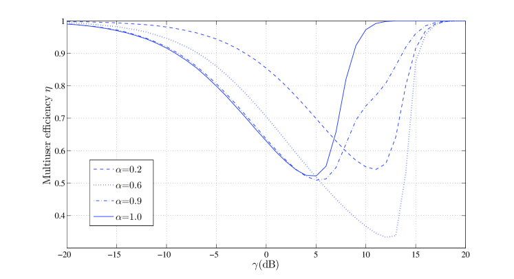
Figure 1: Large-system multiuser efficiency of the user-and-data detector under MAP with prior knowledge of $\alpha$ and $\beta$=3/7.

Our approach differs from that in [9, 19, 8], as the fixed-point equation (13) also includes the prior distribution on the users’ activity in a static channel. Under MAP estimation, detection requires the knowledge not only of the prior information of the data, but also of the activity rate $\alpha$. Thus, the fixed-point equations depend on MMSE, SNR, and system load. Numerical solutions vs. SNR at a load $\beta=3/7$ are shown in Fig. 1. Plots like this one illustrate how the multiuser efficiency is affected by the level of noise and interference, and by the uncertainty in the users’ activity rate. For low SNR, noise dominates, and the performance of the MMSE and the multiuser efficiency is degraded as $\alpha$ grows, since the presence of more active users adds more noise to the system. On the other hand, as we shall discuss later, for high SNR the MMSE strongly depends on the minimum distance between the transmitted symbols, and the activity rate here plays a secondary role. Hence, the gap between the multiuser efficiencies with $\alpha=1$ and $\alpha\neq 1$ for larger SNR is due to the fact that the former constellation has twice the minimum distance of the latter. We can observe clearly the transition behavior from low to high SNR for values of $\alpha$ approaching $1$. Moreover, when $\alpha=1$, (13) reduces to the fixed-point equation for the classical assumption, in which all users are active and transmit a binary antipodal constellation [9]:

$$\eta^{-1}=1+\beta\left(\gamma\left[1-\int\frac{1}{\sqrt{2\pi}}e^{-y^{2}/2}\tanh(\eta\gamma-y\sqrt{\eta\gamma})\textrm{d}y\right]\right).$$ (14)

In this case, it can be shown that, for high SNR, we have $\textrm{MMSE}(\eta\gamma,\alpha=1)\approx\sqrt{\frac{2\pi}{\eta\gamma}}e^{-\eta\gamma/2}$. In fact, the following general result holds:

Lemma III.2

[28] For large output SNR, the MMSE of a system transmitting an equiprobable $M$-ary normalized constellation with minimum Euclidean distance $d$ in a Gaussian channel with noise variance $1/\eta$ is

$$\textrm{MMSE}(\eta\gamma,\alpha=1)=\kappa(\eta\gamma)e^{-d^{2}\eta\gamma/8}$$ (15)

with $\kappa_{1}(\eta\gamma)\leq\kappa(\eta\gamma)\leq\kappa_{2}$, where $\kappa_{1}(\eta\gamma)=\mathcal{O}(1/\sqrt{\eta\gamma})$ and $\kappa_{2}$ is a constant, given by the maximum distance between neighboring symbols.

For the entire range of activity rates, i.e., $\alpha\in[0,1]$, we can derive lower and upper bounds illustrating analytically the transition between the classical assumption ($\alpha=1$) and the cases where the activity is also detected ($\alpha<1$) for large SNR. Our calculations bring about a new analytical framework to deal with large-system analysis, as we will see in the next section. Our bounds are consistent with Lemma III.2 and the lower bound includes the case $\alpha=1$. The general result is stated as follows.

Theorem III.3

The MMSE of joint user identification and data detection in a large system with an unknown number of users has the following behavior, valid for sufficiently large values of the product $\eta\gamma$:

$$2\sqrt{\frac{\alpha(1-\alpha)}{{\pi\eta\gamma}}}e^{-\eta\gamma/8}\leq\textrm{MMSE}(\eta\gamma,\alpha)\leq 2\alpha e^{-\eta\gamma/2}+\sqrt{\frac{\pi\alpha(1-\alpha)}{\eta\gamma}}e^{-\eta\gamma/8}$$ (16)

Proof:

See Appendix B. ∎

Bounds in (16) describe explicitly, in the high-SNR region, the relationship between the MMSE, the users’ activity rate, and the effective SNR ($\eta\gamma$). In Fig. 2 these bounds are compared to the true MMSE values as a function of $\eta\gamma$ for fixed $\alpha$. It can be seen that the uncertainty about the users’ activity modifies substantially the exponential decay of the MMSE for high SNR. In fact, a value of $\alpha$ different from $1$ causes the MMSE to decay by $\exp(-\eta\gamma/8)$, rather than by $\exp(-\eta\gamma/2)$, which would be the case when all users are active. Furthermore, we can observe that, for sufficiently large effective SNR, the behavior vs. $\alpha$ of the optimal detector is symmetric with respect to $\alpha=1/2$, which corresponds to the maximum uncertainty of the activity rate. Figure 3 shows that for large values of the product $\eta\gamma$, the MMSE essentially depends on the minimum distance between the inactivity symbol $\{0\}$ and the data symbols $\{-1,1\}$, and thus users’ identification prevails over data detection. Summarizing, the dependence of the MMSE must be symmetrical with respect to $\alpha=1/2$, since it reflects the impact of prior knowledge about the user’s activity into the estimation.

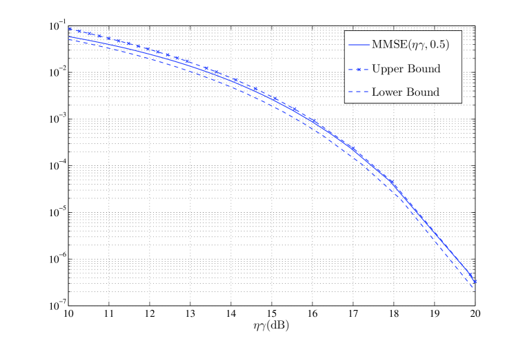
Figure 2: A comparison of the exact MMSE value with its upper and lower bounds for $\alpha=0.5$ and $\eta\gamma\in[10,20]$ dB

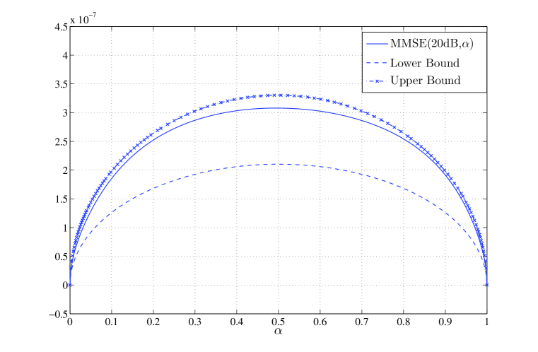
Figure 3: A comparison of the exact MMSE value with its upper and lower bounds for $\eta\gamma=20$ dB and $\alpha\in[0,1]$.

IV Maximum System Load and Related Considerations

Recall the definition of maximum system load $\beta=\frac{K}{N}$, where $K$ is the maximum number of users accessing the multiuser channel. When the number of active users is unknown, and there is a priori knowledge of the activity rate, the actual system load is $\beta^{\prime}=\alpha\beta$. In this section, we focus on $\beta$ and study some of its properties. Notice that, given an activity rate, results for the actual system load follow trivially.

IV-A Solutions to the large-system fixed-point equation

We characterize the behavior of the maximum system load subject to quality-of-service constraints. This helps shedding light into the nature of the solutions of the fixed-point equation (13). In particular, there might be cases where (13) has multiple solutions. These solutions correspond to the solutions appearing in any simple mathematical model of magnetism based on the evaluation of the free energy with the fixed-point method [11]. They represent what in the statistical physics parlance is called phase coexistence (for example, this occurs in ice or liquid phase of water at $0^{\circ}$C). In particular, at low temperatures, the magnetic system might have three solutions $0\leq\Psi_{1}<\Psi_{2}<\Psi_{3}\leq 1$. Solutions $\Psi_{1}$ and $\Psi_{3}$ are stable: one of them is globally stable (it actually minimizes the free energy), whereas the other is metastable, and a local minimum. Solution $\Psi_{2}$ is always unstable, since it is is a local maximum. The “true” solution is therefore given by $\Psi_{1}$ and $\Psi_{3}$, for which the free energy is a minimum. The same consideration applies also to our multiuser detection problem where multiuser efficiencies for the IO detector might vary significantly depending on the value of the system load and SNR. More specifically, for sufficiently large SNR, stable solutions may switch between a region that approaches the single-user performance ($\eta=1-\epsilon_{1}$) and a region approaching the worst performance ($\eta=\epsilon_{0}$), for $0<\epsilon_{1},\epsilon_{0}\ll 1$. Following previous literature [8], we shall call the former solutions good and the latter bad. When the solution is unique, due to low or high system load, the multiuser efficiency is a globally stable solution that lies in either the good or the bad solution region. Then, for given system parameters, the set of operational (or globally stable) solutions is formed by solutions that are part of these sets and minimize the free energy.

The existence of good and bad solutions are critical in our problem. From a computational perspective, we are particularly interested in single solutions, either bad or good, that surely avoid metastability and instability. These solutions belong to a specific subregion within the bad and good regions, and appear for low and high SNR, respectively. From an information-theoretic perspective, it might seem that the true solutions should capture all our attention. However, it has been shown that metastable solutions appear in suboptimal belief-propagation-based multiuser detectors, where the system is easily attracted into the bad solutions region (corresponding to low multiuser efficiency), due to initial configurations that are far from the true solution [12]. Moreover, the region of good solutions is of interest in the high-SNR analysis, because, for a given system load, it can be observed that the multiuser efficiency tends to $1$, consistently with previous theoretical results [22]. In what follows, we provide an analysis of the boundaries of the stable solution regions, as well as their computationally feasible subregions with practical interest in the low and high SNR regimes.

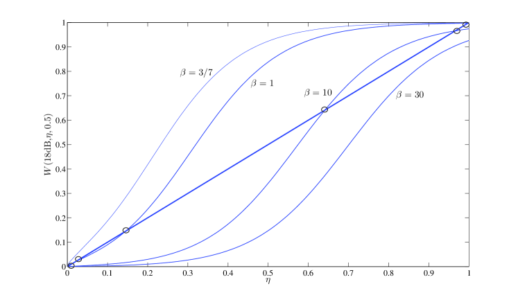
Figure 4: Fixed-point solutions (marked by circles) for different values of $\beta$ and fixed $\alpha=0.5$, and $\gamma=18$ dB.

A quantitative illustration of the above considerations is provided by plotting the left- and right-hand sides of (13) to obtain fixed points for constant values of amplitude and activity rate, and as a function of the system load. The solutions of (13) are found at the intersection of the curve corresponding to the right-hand side with the $y=\eta$ line. Fig. 4 plots different solutions of the right-hand side of (13) for increasing system load, $\alpha=0.5$ and $\gamma=18$ dB:

$$W(\gamma,\eta,\alpha)\triangleq\frac{1}{1+\beta\gamma\rm{MMSE}(\eta\gamma,\alpha)}$$

Notice first that the structure of the fixed-point equation in general does not allow the solution $\eta=0$, and for finite $\gamma$ and $\beta$, $\eta=1$ is not a solution. In fact, the latter is an asymptotic solution for large SNR and certain system loads, as the MMSE decays exponentially to $0$. From Fig. 4, one can observe the presence of phase transitions and the coexistence of multiple solutions. In particular, we observe that for $\beta=3/7$ the good solution is computationally feasible. On the other hand, for $\beta=1$ and $\beta=10$ the system has three solutions, where the true solution belongs to either the bad or the good solution region. When the system load achieves $\beta=30$, the curve only intersects the identity curve near $0$, and the operational solution is unique and lies in a subregion of bad solutions.

IV-B System load and the space of fixed-point solutions

Even in the case of good solutions, the multiuser efficiency can be greatly degraded by the joint effect of the activity rate and the maximum system load. In order to analyze the fixed-point equation (13) from a different perspective and shed light into the interplay between these parameters, we express the maximum system load as the following function, derived from (13):

$$\Upsilon_{\beta}(\gamma,\eta,\alpha)\triangleq\frac{\left(1-\eta\right)}{\eta\gamma\textrm{MMSE}(\eta\gamma,\alpha)}$$ (17)

Since MMSE is a continuous function of $\eta$ [10], then $\Upsilon_{\beta}$ is also a continuous function in any compact set over the domain $\eta\in(0,1]$ for given SNR and activity rate. It is also easy to observe that, for small values of $\eta$, $\Upsilon_{\beta}$ tends to infinity regardless of $\gamma$ and $\alpha$, whereas in the high-$\eta$ region, which is of interest here, it decays to $0$. Before analyzing the behavior of (17), we introduce a few definitions that help describe the boundaries between the regions with and without coexistence (in the statistical-physics literature, these boundaries are called spinodal lines [8]). We also define appropriately the regions of potentially stable solutions as introduced before.

Definition IV.1

The critical system load $\beta^{\star}(\gamma,\alpha)$ is the maximum load at which a stable good solution of (13) exists.

Definition IV.2

The transition system load $\beta_{\star}(\gamma,\alpha)$ is the minimum load at which the true solution of (13), $\eta_{\star}$ coexists with other solutions $\eta_{\star}^{\prime}$.

Definition IV.3

The good solution region corresponds to the domain of (17) formed by the maximum $\eta$ in every set of pre-images of $\Upsilon_{\beta}$ below the critical system load:

$$\mathcal{R}_{g}=\left\{\eta\in[0,1],\eta=\max\{\Upsilon_{\beta}^{-1}(\beta)\},\forall\beta\in[0,\beta^{\star}]\right\}$$ (18)

Similarly, the bad solution region corresponds to the domain of (17) formed by the minimum $\eta$ in every set of pre-images of $\Upsilon_{\beta}$ above the transition system load:

$$\mathcal{R}_{b}=\left\{\eta\in[0,1],\eta=\min\{\Upsilon_{\beta}^{-1}(\beta)\},\forall\beta\in[\beta_{\star},+\infty)\right\}$$ (19)

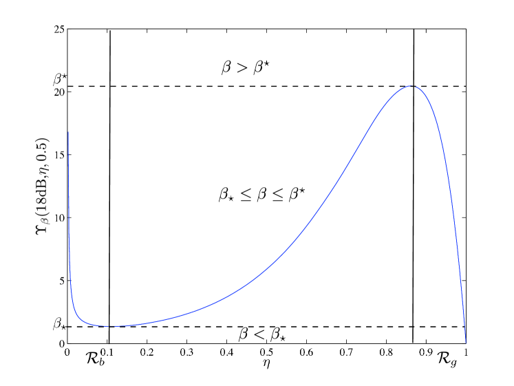
Figure 5: System load function in the multiuser efficiency domain for $\alpha=0.5$ and $\gamma=18$ dB.

Fig. 5 illustrates $\Upsilon_{\beta}$ (for fixed SNR and activity rate) and show the regions defined by the aforementioned parameters. It is important to remark that both system loads defined above delimit the regions from which there is phase coexistence ($\beta_{\star}\leq\beta\leq\beta^{\star}$) from the areas where there is one solution ($\beta>\beta^{\star}$ or $\beta<\beta_{\star}$). Additionally, Fig. 5 illustrates the set of solutions that satisfy conditions (18), (19).

Fig. 5 illustrates that it seems useful to define analytically the domain where stable solutions can be found. Beforehand, we differentiate for convenience the case with unknown number of users $\alpha\in(0,1)$, from the case where all users are active ($\alpha=1$). We do not consider the case $\alpha=0$.

IV-B1 Case $\alpha\in(0,1)$

In order to analyze the conditions on the system load, SNR, and activity rate, for which we can find a good solution, we use the asymptotic results on the MMSE (16), yielding lower and upper bounds $L(.)\leq\Upsilon_{\beta}(\gamma,\eta,\alpha)\leq U(.)$ for large enough $\eta\gamma$, where

$$L(\gamma,\eta,\alpha) \triangleq \frac{\left(1-\eta\right)}{\sqrt{\pi\eta\gamma\alpha(1-\alpha)}}e^{\eta\gamma/8}$$ (20)

$$U(\gamma,\eta,\alpha) \triangleq \frac{\left(1-\eta\right)}{2}\sqrt{\frac{\pi}{\eta\gamma\alpha(1-\alpha)}}e^{\eta\gamma/8}$$ (21)

Although not exact for low SNR, the dependence on $\eta$ of the upper and lower bound provides a good approximation for the dependence of $\Upsilon_{\beta}$ for large SNR and given $\alpha$. Hence, by using $U(.)$ and $L(.)$, we obtain necessary and sufficient conditions that determine the regions of stable solutions and provide analytical expressions for the transition and critical system loads. The main result for $\alpha\in(0,1)$ follows:

Theorem IV.4

Given the range of activity rates $\alpha\in(0,1)$, a necessary condition for phase coexistence is

$$\gamma\geq 4(3+2\sqrt{2}),\quad(\gamma\geq 13.67\;\textrm{dB})$$ (22)

Moreover, for high SNR, the condition is met and the transition system load is bounded by

$$L(\gamma,\eta_{m},\alpha)<\beta_{\star}(\gamma,\alpha)<U(\gamma,\eta_{m},\alpha)$$ (23)

while the critical system load is bounded by

$$L(\gamma,\eta_{M},\alpha)<\beta^{\star}(\gamma,\alpha)<U(\gamma,\eta_{M},\alpha)$$ (24)

and $\eta_{m}$, $\eta_{M}$ are given by

$$\eta_{m} \triangleq (\gamma/2-2-4\Delta(\gamma))/\gamma$$

$$\eta_{M} \triangleq (\gamma/2-2+4\Delta(\gamma))/\gamma$$

where $\Delta(\gamma)=\sqrt{(\gamma/8)^{2}-3\gamma/8+1/4}$.

Hence, the bad-solution region is given by $\mathcal{R}_{b}=(0,\eta_{m}]$, whereas the good-solution region is $\mathcal{R}_{g}=[\eta_{M},1]$. Similarly, the subregions of single bad solutions, that we shall denote $R_{bc}=(0,\eta_{bc})\subset\mathcal{R}_{b}$, and of single good solutions, denoted by $R_{gc}=(\eta_{gc},1]\subset\mathcal{R}_{g}$, satisfy

$$\eta_{bc} = \min\{\Upsilon_{\beta}^{-1}(\beta^{\star})\}>\eta^{\star}_{bc}$$

$$\eta_{gc} = \max\{\Upsilon_{\beta}^{-1}(\beta_{\star})\}<\eta^{\star}_{gc}$$

where $\eta^{\star}_{bc}\triangleq\min\{U^{-1}(\beta^{\star})\}$, and $\eta^{\star}_{gc}\triangleq\max\{L^{-1}(\beta^{\star})\}$ are obtained from the bounds.

Proof:

See Appendix C. ∎

The above result provides the general boundaries of the space of solutions of our problem. It is important to note that $\eta_{m}$ and $\eta_{M}$ are very good approximations for high SNR of the positions of the minimum and maximum observed in Fig. 5, which determine the transition and the critical system loads. As a consequence, remark that Theorem IV.4 analytically tells us the range of $\beta$’s for which there are either single or multiple solutions based on the up-to-a-constant approximation of $\Upsilon_{\beta}$ by (20) and (21). Similarly, $\eta^{*}_{bc}$ and $\eta^{*}_{gc}$ are tight bounds of the boundaries of the single-solution regions as $U(.)$ and $L(.)$ are of $\Upsilon_{\beta}(.)$. Note also that the activity rate affects the boundaries in the same symmetrical manner as it does the MMSE (i.e., the worst case here also corresponds to $\alpha=0.5$) but has no impact on the operational region, that is only reduced in size by increasing the SNR. In particular, these regions are characterized, in the limit of high SNR, as follows:

Corollary IV.5

In the limit of high SNR, $\mathcal{R}_{g}\to\{1\}$, $\mathcal{R}_{b}\to\{0\}$, and consequently $\mathcal{R}_{gc}\to\{1\}$, and $\mathcal{R}_{bc}\to\{0\}$ .

Proof:

The above corollary results from

$$\lim_{\gamma\to\infty}\eta_{M} = \lim_{\gamma\to\infty}\frac{(\gamma/2-2+4\sqrt{(\gamma/8)^{2}-3\gamma/8+1/4})}{\gamma}=1$$

$$\lim_{\gamma\to\infty}\eta_{m} = \lim_{\gamma\to\infty}\frac{(\gamma/2-2-4\sqrt{(\gamma/8)^{2}-3\gamma/8+1/4})}{\gamma}=0$$

∎

Note that, given a system load $\beta$ with $\beta^{\star}>\beta$, for sufficiently large SNR the unique true (large-system) solution is $\eta=1$, which corroborates the main result in [22]. Moreover, the description of the feasible good solutions by analytical means allows the computation of a sufficient condition on the system load to guarantee a given multiuser efficiency in practical implementations. More specifically, we use the aforementioned lower bound on $\Upsilon$ to state that any system load below $L(.)$ guarantees that the given multiuser efficicency is achieved. The result is stated as follows:

Corollary IV.6

The maximum system load, $\beta_{\alpha,\eta}$, for a given activity rate and multiuser efficiency requirement, $\eta=1-\epsilon$, where $0<\epsilon\ll 1$, that lies in $R_{gc}$, is lower-bounded in the high-SNR region by

$$\beta_{\alpha,\eta}>\frac{\epsilon}{\sqrt{\pi\eta\gamma\alpha(1-\alpha)}}e^{(1-\epsilon)\gamma/8}.$$ (25)

In Fig. 6 we show the numerical values of the transition and the critical system load as a function of the SNR in the $(\gamma,\beta)$ space. We also use the asymptotic expansion to derive upper and lower bounds, respectively. The plotted curves are the spinodal lines, which mark the boundary between the regions with and without solution coexistence. The $\beta_{\star}$ (lower branch) separates the region where the bad solution disappears, whereas $\beta^{\star}$ (upper branch) contains the bifurcation points at which the operational solution disappears. The intersection point between both branches corresponds to the SNR threshold (22), which provides the necessary condition for solution coexistence.

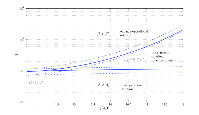
Figure 6: Upper and lower bounds on the numerical spinodal lines (thick line) for $\alpha=0.5$.

IV-B2 Case $\alpha=1$

We now apply the same reasoning for the “classical” approach to multiuser detection, corresponding to activity rate $1$. In this case, using the approximation in [28], the system load function can be lower-bounded by

$$\Upsilon_{\beta}(\gamma,\eta,1)=\frac{\left(1-\eta\right)}{\eta\gamma\textrm{MMSE}(\eta\gamma,1)}<\frac{\left(1-\eta\right)e^{\eta\gamma/2}}{\sqrt{\pi\eta\gamma}}$$ (26)

Hence, we can derive the following spinodal lines

Corollary IV.7

Given $\alpha=1$ a necessary condition for the phase coexistence is that

$$\gamma\geq 3+2\sqrt{2},\quad(\gamma\geq 7.65\textrm{dB}).$$

Moreover, for high SNR, the condition is met and the transition system load is upper-bounded by

$$\beta_{\star}<\frac{\left(1-\eta_{m^{\prime}}\right)}{2}\sqrt{\frac{\pi}{\eta_{m^{\prime}}\gamma}}e^{\frac{\eta_{m^{\prime}}\gamma}{2}}$$ (27)

and the critical system load is upper-bounded by

$$\beta^{\star}<\frac{\left(1-\eta_{M^{\prime}}\right)}{2}\sqrt{\frac{\pi}{\eta_{M^{\prime}}\gamma}}e^{\frac{\eta_{M^{\prime}}\gamma}{2}}$$ (28)

where $\eta_{m^{\prime}}$ and $\eta_{M^{\prime}}$ are given by

$$\eta_{m^{\prime}} \triangleq \frac{(\gamma/2-1/2-\Lambda(\gamma))}{\gamma}$$

$$\eta_{M^{\prime}} \triangleq \frac{(\gamma/2-1/2+\Lambda(\gamma))}{\gamma}$$

and $\Lambda(\gamma)=\sqrt{(\gamma/2)^{2}-3\gamma/2+1/4}$.

Hence, the bad solution region is given by $\mathcal{R}_{b}=(0,\eta_{m^{\prime}}]$ whereas the good solution region is $\mathcal{R}_{g}=[\eta_{M^{\prime}},1]$.

Proof:

The proof is analogous to that of Theorem IV.4. ∎

The same consequence for the asymptotic operational region holds here.

Corollary IV.8

In the limit of high SNR, $\mathcal{R}_{g}\to\{1\}$, and $\mathcal{R}_{b}\to\{0\}$.

Proof:

This corollary results from

$$\lim_{\gamma\to\infty}\eta_{M}=\lim_{\gamma\to\infty}\frac{(\gamma/2-1/2+\sqrt{(\gamma/2)^{2}-3\gamma/2+1/4})}{\gamma}=1$$

$$\lim_{\gamma\to\infty}\eta_{m}=\lim_{\gamma\to\infty}\frac{(\gamma/2-1/2-\sqrt{(\gamma/2)^{2}-3\gamma/2+1/4})}{\gamma}=0$$

∎

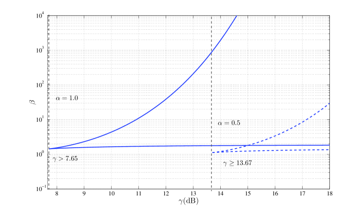
Figure 7: Comparison of upper bounds on the spinodal lines for $\alpha=1.0$ (left) and $\alpha=0.5$ (right).

In Fig. 7, one can observe a $6$ dB-difference between the spinodal lines corresponding to $\alpha=0.5$ and to $\alpha=1.0$. This is due to the minimum distance of the underlying constellations, which causes the MMSE to have different exponential decays. This can be interpreted by saying that the addition of activity detection to data detection is reflected by a $6$ dB increase of the SNR needed to achieve the same system load performance. Moreover, with $\alpha<1$, the transition system load is lower than the case where all users are active, and, therefore, computationally good solutions correspond to lower values of the maximum system load.

IV-C Maximum system load with error probability constraints

A natural application of the above results to practical designs appears when the quality-of-service requirements of the system are specified in terms of uncoded error probability. Such an application can provide some extra insight into the plausible values of $\beta$ with joint activity and data detection for efficient design of large CDMA systems. Once a multiuser-efficiency requirement is assigned, the corresponding probability of error follows naturally. Note first that, in order to detect the activity as well as the transmitted data, our model deals with a ternary constellation $\{-1,0,1\}$. When any of these symbols is transmitted by each user with constant SNR$=\gamma$ through a bank of large-system equivalent white Gaussian noise channels with variance $1/\eta$, the probability of error over $\mathcal{X}$ depends on the prior probabilities as well as the Euclidean distance between the symbols. The error probability implied by the replica analysis is

$$P_{e}(\eta,\gamma,\alpha)=2(1-\alpha)Q\left(\frac{\sqrt{\eta\gamma}}{2}+\frac{\lambda_{\alpha}}{\sqrt{\eta\gamma}}\right)+\alpha Q\left(\frac{\sqrt{\eta\gamma}}{2}-\frac{\lambda_{\alpha}}{\sqrt{\eta\gamma}}\right)$$ (29)

where $Q(x)\triangleq\frac{1}{\sqrt{2\pi}}\int_{x}^{\infty}e^{-\frac{t^{2}}{2}}dt$ is the Gaussian tail function, and $\lambda_{\alpha}\triangleq\ln\left(\frac{2(1-\alpha)}{\alpha}\right)$.

The relationship between $\eta$ and $P_{e}$ for our particular case can be used to reformulate the bounds on the function $\Upsilon_{\beta}$ in terms of error probability.

Corollary IV.9

The maximum system load, $\Upsilon_{\beta}(\eta,\gamma,\alpha)$, for a given error probability $P_{e}$, $\gamma$, and activity rate is bounded for high SNR by:

$$L(\gamma,\eta_{\textrm{max}},\alpha)<\Upsilon_{\beta}(\eta_{\textrm{max}},\gamma,\alpha)<U(\gamma,\eta_{\textrm{max}},\alpha)$$ (30)

where

$$\eta_{\textrm{max}}\triangleq\max\left\{\eta_{P},\eta_{gc}\right\},$$

and $(\eta_{P},\gamma,\alpha)$ is the pre-image of $P_{e}$.

Proof:

The result is obtained by noticing that the multiuser efficiency requirement extracted from $P_{e}$ must lie on the subregion $(\eta_{gc},1]$. ∎

Notice that, if the error probability satisfies $\eta_{p}\leq\eta_{gc}=\eta_{\textrm{max}}$, then the constraint is described by the bounds on the transition load (24). However, if $\eta_{gc}<\eta_{p}=\eta_{\textrm{max}}$, then, for Corollary IV.6, the maximum system load can be also easily bounded. Fig. 8 plots the critical system load for two different error probabilities requirements and three different activity rates.

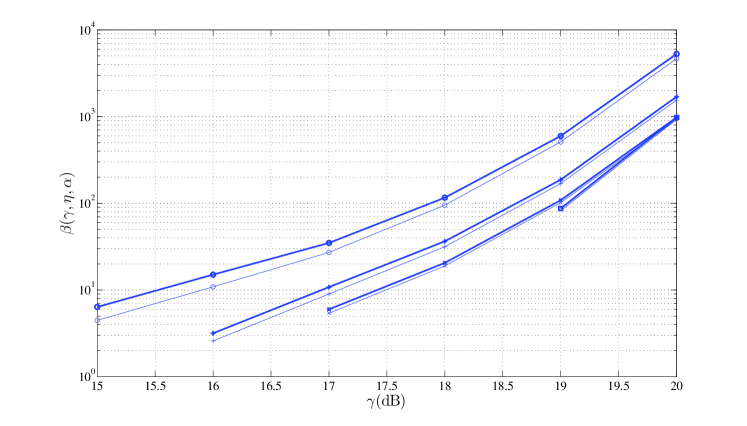
Figure 8: Critical system load for different uncoded error probabilities and activity rates. Thicker lines represent numerical results, whereas regular lines show the corresponding lower bounds. Lines with circle markers: $P_{e}=10^{-3}$ and $\alpha=0.99$. Lines with cross markers: $P_{e}=10^{-3}$ and $\alpha=0.1$. Lines with star markers: $P_{e}=10^{-3}$ and $\alpha=0.5$. Lines with square markers: error probability $10^{-5}$ and $\alpha=0.5$.

V Conclusions

We have analyzed multiuser detectors for CDMA where the fraction of active users is unknown, and must be estimated in a tracking phase. Using a large-system approach and statistical-physics tools, we have derived a fixed-point equation for the optimal user-and-data detector, and provided asymptotic bounds for the corresponding MMSE. Further, we have described the space of stable solutions of the fixed-point equation, and derived explicit bounds on the critical and transition system loads for all users’ activity rates. These are consistent with the results obtained under the classic multiuser-detection assumption ($\alpha=1.0$) made in the literature. The study of the so-called spinodal lines allowed us to determine the regions of stable good and bad solutions, including subregions of single solutions (also computationally feasible), in the system load vs. SNR parameter space of our model. Our results show that for a user-and-data detector, the boundaries of the space of solutions do depend on the activity rate, whereas the regions of stable solutions (good and bad) are only affected by the SNR. Hence, the overall system load performance keeps a symmetric behavior with respect to $\alpha$. In practical implementations with high quality-of-service demands, we are interested in maximizing the critical system load, while keeping the optimal detector in the feasible subregion of good multiuser efficiencies, such that a a wider range of potential users can successfully access the channel with a given rate. By increasing the SNR, this goal can be achieved, but for limited SNR, the certainty on the users’ activity allows allocation of more users for a given spreading length. A relevant example corresponds to a system with a given error probability requirement. For this case, we have shown that, for sufficiently large SNR, we can choose the minimum multiuser efficiency in the domain of feasible good solutions, and maximize the critical system load regardless of the error probability target.

One of the assumptions of this paper is to model the activity as an i.i.d. process. Further extensions of this work to non-i.i.d scenarios can be found in [5] where the users’ activity evolves according to a Markov process and in [29], where users transmit encoded messages and the activity is correlated over the coded blocks of each user.

Appendix A Proof of Corollary III.1

We first derive the MMSE for our particular ternary input distribution in the general fixed-point equation (9):

$$\textrm{MMSE}(\eta\gamma,\alpha) =\mathbb{E}\left[\biggl{(}{\boldsymbol{b}}^{k}-\mathbb{E}\{{\boldsymbol{b}}^{k}|{\boldsymbol{S}},y\}\biggl{)}^{2}\right]$$

$$=\alpha-\int\frac{\mathbb{E}_{{\boldsymbol{b}}^{k}}^{2}\{{\boldsymbol{b}}^{k}P(y|\eta,{\boldsymbol{b}}^{k},S)\}}{\mathbb{E}_{{\boldsymbol{b}}^{k}}\{P(y|\eta,{\boldsymbol{b}}^{k},S)\}}\textrm{d}y$$

$$=\alpha-\int\frac{\left(\sqrt{\frac{\eta}{2\pi}}\frac{\alpha}{2}\left[e^{-\frac{\eta}{2}(y-\sqrt{\gamma})^{2}}-e^{-\frac{\eta}{2}(y+\sqrt{\gamma})^{2}}\right]\right)^{2}}{\sqrt{\frac{\eta}{2\pi}}\left(\frac{\alpha}{2}\left[e^{-\frac{\eta}{2}(y-\sqrt{\gamma})^{2}}+e^{-\frac{\eta}{2}(y+\sqrt{\gamma})^{2}}\right]\right)+(1-\alpha)e^{\frac{\eta}{2}y^{2}}}\textrm{d}y$$

$$=\alpha-\frac{1}{2}\sqrt{\frac{\eta}{2\pi}}\left[\int\frac{e^{-\frac{\eta}{2}(y-\sqrt{\gamma})^{2}}\alpha^{2}\sinh(\eta y\sqrt{\gamma})}{\alpha\cosh(\eta y\sqrt{\gamma})+(1-\alpha)e^{\frac{\eta\gamma}{2}}}\textrm{d}y-\int\frac{e^{-\frac{\eta}{2}(y^{\prime}+\sqrt{\gamma})^{2}}\alpha^{2}\sinh(\eta y^{\prime}\sqrt{\gamma})}{\alpha\cosh(\eta y^{\prime}\sqrt{\gamma})+(1-\alpha)e^{\frac{\eta\gamma}{2}}}\textrm{d}y^{\prime}\right].$$

After appropriate change of variables

the MMSE is

$$\rm{MMSE}(\eta\gamma,\alpha) =\alpha-\int\frac{1}{\sqrt{2\pi}}e^{\frac{-y^{2}}{2}}\frac{\alpha^{2}\sinh[\eta\gamma-y\sqrt{\eta\gamma}]}{\alpha\cosh[\eta\gamma-y\sqrt{\eta\gamma}]+(1-\alpha)e^{\eta\gamma/2}}\textrm{d}y$$

Since the SNR is constant among users, it follows naturally that the large-system fixed-point equation is given by (13).

Appendix B Proof of Theorem III.3

From now on, we omit the explicit indication of the arguments of the MMSE function. The lower bound is obtained by noting that, for large SNR, the general MMSE, denoted $\textrm{MMSE}_{\alpha}$, is lower-bounded by $\textrm{MMSE}_{\{0,1\}}$, which describes the detection performance when the transmitted symbols are $\{0,1\}$, with probabilities $\{1-\alpha,\alpha\}$. In this case the MMSE has the following form

$$\textrm{MMSE}_{\{0,1\}} =\alpha-\int\frac{\left(\sqrt{\frac{\eta}{2\pi}}\alpha e^{-\frac{\eta}{2}(y-\sqrt{\gamma})^{2}}\right)^{2}}{\sqrt{\frac{\eta}{2\pi}}\left(\alpha e^{-\frac{\eta}{2}(y-\sqrt{\gamma})^{2}}+(1-\alpha)e^{-\frac{\eta}{2}y^{2}}\right)}\textrm{d}y$$

where $\lambda_{\alpha}\triangleq\frac{1}{2}\ln\left(\frac{1-\alpha}{\alpha}\right)$. After some manipulation and appropriate changes of variables, we obtain

$$\textrm{MMSE}_{\{0,1\}} =\alpha-\alpha e^{-\frac{3\eta\gamma}{8}-\lambda_{\alpha}}\sqrt{\frac{1}{2\pi}}\int_{-\infty}^{\infty}e^{-\frac{1}{2}(2z-\sqrt{\eta\gamma}+\frac{2\lambda_{\alpha}}{\sqrt{\eta\gamma}})^{2}}\operatorname{sech}\left(z\sqrt{\eta\gamma}\right)\textrm{d}z.$$

Use now the following asymptotic expansion for $\operatorname{sech}(z)$: $\left|z\right|\to\infty$

$$\operatorname{sech}(z)=2e^{-\left|z\right|}\left(1+\sum_{\ell=1}^{\infty}(-1)^{\ell}e^{-2\ell\left|z\right|}\right)$$

and obtain

$$\textrm{MMSE}_{\{0,1\}}=\alpha-\alpha e^{-\frac{3\eta\gamma}{8}-\lambda_{\alpha}}\sqrt{\frac{1}{2\pi}}\Biggl{[} \int_{-\infty}^{0}e^{-\frac{1}{2}(2z-\sqrt{\eta\gamma}+\frac{2\lambda_{\alpha}}{\sqrt{\eta\gamma}})^{2}}2e^{z\sqrt{\eta\gamma}}\left(1+\sum_{\ell=1}^{\infty}(-1)^{\ell}e^{2\ell z\sqrt{\eta\gamma}}\right)\textrm{d}z$$

$$+ \int_{0}^{\infty}e^{-\frac{1}{2}(2z-\sqrt{\eta\gamma}+\frac{2\lambda_{\alpha}}{\sqrt{\eta\gamma}})^{2}}2e^{-z\sqrt{\eta\gamma}}\left(1+\sum_{\ell=1}^{\infty}(-1)^{\ell}e^{-2\ell z\sqrt{\eta\gamma}}\right)\textrm{d}z\Biggl{]}.$$

We now use the expansion

$$\textrm{MMSE}_{\{0,1\}}=\alpha-\alpha e^{-\eta\gamma/8+\lambda_{\alpha}-\frac{2\lambda^{2}_{\alpha}}{\eta\gamma}}\Biggl{[} \sum_{\ell=0}^{\infty}(-1)^{\ell}\sqrt{\frac{2}{\pi}}\int_{-\infty}^{0}e^{-2z^{2}+\left((3+2\ell)\sqrt{\eta\gamma}-\frac{4\lambda_{\alpha}}{\sqrt{\eta\gamma}}\right)z}\textrm{d}z$$

$$+ \sum_{\ell=0}^{\infty}(-1)^{\ell}\sqrt{\frac{2}{\pi}}\int_{0}^{\infty}e^{-2z^{2}+\left((1-2\ell)\sqrt{\eta\gamma}-\frac{4\lambda_{\alpha}}{\sqrt{\eta\gamma}}\right)z}\textrm{d}z\Biggl{]}.$$

Express now the integrals in terms of the Q-function, $Q(x)\triangleq\frac{1}{\sqrt{2\pi}}\int_{x}^{\infty}e^{-\frac{t^{2}}{2}}dt$

$$\textrm{MMSE}_{\{0,1\}}=\alpha e^{-\eta\gamma/8+\lambda_{\alpha}-\frac{2\lambda^{2}_{\alpha}}{\eta\gamma}} \Biggl{[}e^{\frac{\left(\frac{\sqrt{\eta\gamma}}{2}-\frac{2\lambda_{\alpha}}{\sqrt{\eta\gamma}}\right)^{2}}{2}}Q\left(\frac{\sqrt{\eta\gamma}}{2}-\frac{2\lambda_{\alpha}}{\sqrt{\eta\gamma}}\right)-e^{\frac{\left(\frac{3\sqrt{\eta\gamma}}{2}-\frac{2\lambda_{\alpha}}{\sqrt{\eta\gamma}}\right)^{2}}{2}}Q\left(\frac{3\sqrt{\eta\gamma}}{2}-\frac{2\lambda_{\alpha}}{\sqrt{\eta\gamma}}\right)$$

$$-\sum_{\ell=1}^{\infty}(-1)^{\ell}\biggl{[}e^{\frac{\left(\frac{(2\ell-1)\sqrt{\eta\gamma}}{2}+\frac{2\lambda_{\alpha}}{\sqrt{\eta\gamma}}\right)^{2}}{2}}Q\left(\frac{(2\ell-1)\sqrt{\eta\gamma}}{2}+\frac{2\lambda_{\alpha}}{\sqrt{\eta\gamma}}\right)$$

$$+e^{\frac{\left(\frac{(3+2\ell)\sqrt{\eta\gamma}}{2}-\frac{2\lambda_{\alpha}}{\sqrt{\eta\gamma}}\right)^{2}}{2}}\left(Q\left(\frac{(3+2\ell)\sqrt{\eta\gamma}}{2}-\frac{2\lambda_{\alpha}}{\sqrt{\eta\gamma}}\right)\right)\biggl{]}\Biggl{]}.$$

Next, use the expansion of the Q function, [1]:

$$Q(x)=\frac{e^{-x^{2}/2}}{\sqrt{2\pi}x}\left(1+\sum_{\ell=1}^{\infty}(-1)^{\ell}\frac{\prod_{q=1}^{\ell}(2q-1)}{x^{2\ell}}\right)$$ (31)

to obtain

$$\textrm{MMSE}_{\{0,1\}}=2\sqrt{\frac{\alpha(1-\alpha)}{2\pi\eta\gamma}}e^{-\eta\gamma/8-\frac{2\lambda^{2}_{\alpha}}{\eta\gamma}}\Biggl{[} \frac{1}{\left(1-\frac{4\lambda_{\alpha}}{\eta\gamma}\right)}+\frac{1}{\left(1+\frac{4\lambda_{\alpha}}{\eta\gamma}\right)}-\frac{1}{\left(3-\frac{4\lambda_{\alpha}}{\eta\gamma}\right)}-\frac{1}{\left(3+\frac{4\lambda_{\alpha}}{\eta\gamma}\right)}$$

$$+\dots+\mathcal{O}\left(\frac{1}{\sqrt{\eta\gamma}}\right)\Biggl{]}$$

where the linear term in $\lambda_{\alpha}$ is substituted in the common factor. Assuming a large value $\eta\gamma$, and using the result

$$2\sum_{n=0}^{\infty}\frac{(-1)^{n+1}}{2n+1}=\frac{\pi}{2}$$

we obtain the following lower bound

$$\textrm{MMSE}_{\{0,1\}}>2\sqrt{\frac{\alpha(1-\alpha)}{2\pi\eta\gamma}}e^{-\eta\gamma/8} \sqrt{2}=2\sqrt{\frac{\alpha(1-\alpha)}{\pi\eta\gamma}}e^{-\eta\gamma/8}.$$

As far as the upper-bound is concerned, we derive the general MMSE, denoted $\textrm{MMSE}_{\alpha}$, and its particular case when all users are assumed to be active, denoted $\textrm{MMSE}_{1}$. Hence, we express the corresponding integrals in an analogous manner

$$\zeta_{\alpha} = \int\frac{1}{\sqrt{2\pi}}e^{\frac{-(y-\sqrt{\eta\gamma})^{2}}{2}}\frac{\alpha\sinh(y\sqrt{\eta\gamma})}{\alpha\cosh(y\sqrt{\eta\gamma})+(1-\alpha)e^{\eta\frac{\gamma}{2}}}\textrm{d}y.$$

$$\zeta_{1} = \int\frac{1}{\sqrt{2\pi}}e^{\frac{-(y-\sqrt{\eta\gamma})^{2}}{2}}\tanh(y\sqrt{\eta\gamma})\textrm{d}y.$$

We now obtain

$$\textrm{MMSE}_{\alpha} =\alpha(1-\zeta_{\alpha})=\alpha\left(1+\zeta_{1}-\zeta_{1}-\zeta_{\alpha}\right)=\alpha\left((1-\zeta_{1})+(\zeta_{1}-\zeta_{\alpha})\right)$$

$$=\alpha\left(\textrm{MMSE}_{1}+(\zeta_{1}-\zeta_{\alpha})\right)$$

Next, we expand $\alpha(\zeta_{1}-\zeta_{\alpha})$, which yields

$$\alpha(\zeta_{1}-\zeta_{\alpha}) =(1-\alpha)e^{\eta\gamma/2}\int\frac{1}{\sqrt{2\pi}}e^{\frac{-(y-\sqrt{\eta\gamma})^{2}}{2}}\frac{\alpha\sinh[y\sqrt{\eta\gamma}]}{\alpha\cosh^{2}[y\sqrt{\eta\gamma}]+(1-\alpha)e^{\eta\gamma/2}\cosh(y\sqrt{\eta\gamma})}\textrm{d}y$$

$$=(1-\alpha)e^{\eta\gamma/2}\int\frac{1}{\sqrt{2\pi}}e^{\frac{-(y-\sqrt{\eta\gamma})^{2}}{2}}\frac{\tanh[y\sqrt{\eta\gamma}]}{\cosh[y\sqrt{\eta\gamma}]+e^{\eta\gamma/2+\ln\left(\frac{1-\alpha}{\alpha}\right)}}\textrm{d}y$$ (32)

Consider now the following inequalities

$$\tanh(z)\leq 1\quad\text{and}\quad\cosh(z)\geq\frac{e^{z}}{2}$$

After substitution and manipulation of the denominator of (32), we obtain

$$\alpha\left(\zeta_{1}-\zeta_{\alpha}\right)\leq (1-\alpha)e^{\eta\gamma/2}\int_{-\infty}^{\infty}\frac{e^{\frac{-(y-\sqrt{\eta\gamma})^{2}}{2}}}{\sqrt{2\pi}}\frac{1}{\frac{e^{y\sqrt{\eta\gamma}}}{2}+e^{\eta\gamma/2+\ln\left(\frac{(1-\alpha)}{\alpha}\right)}}\textrm{d}y$$

$$= (1-\alpha)e^{\eta\gamma/2}\int_{-\infty}^{\infty}\frac{e^{\frac{-(y-\sqrt{\eta\gamma})^{2}}{2}}}{\sqrt{2\pi}}\frac{e^{-\frac{y\sqrt{\eta\gamma}}{2}-\frac{\eta\gamma}{4}-\phi_{\alpha}}}{\cosh\left(\frac{y\sqrt{\eta\gamma}}{2}-\frac{\eta\gamma}{4}-\phi_{\alpha}\right)}\textrm{d}y,$$

where $\phi_{\alpha}\triangleq\frac{1}{2}\ln\left(\frac{2(1-\alpha)}{\alpha}\right)$. We readjust terms to express the integral in a convenient form

$$\alpha\left(\zeta_{1}-\zeta_{\alpha}\right)\leq(1-\alpha)e^{-\eta\gamma/8-\phi_{\alpha}}\int_{-\infty}^{\infty}\frac{e^{\frac{-\left(y-\frac{\sqrt{\eta\gamma}}{2}\right)^{2}}{2}}}{\sqrt{2\pi}}\operatorname{sech}\left(\frac{y\sqrt{\eta\gamma}}{2}-\frac{\eta\gamma}{4}-\phi_{\alpha}\right)\textrm{d}y.$$

We now use the following transformation in the variable of integration: $y=2z+\frac{\sqrt{\eta\gamma}}{2}+\frac{2\phi_{\alpha}}{\sqrt{\eta\gamma}}$.

$$\alpha\left(\zeta_{1}-\zeta_{\alpha}\right)\leq 2(1-\alpha)e^{\frac{7\eta\gamma}{8}-\phi_{\alpha}}\int_{-\infty}^{0}\frac{e^{\frac{-\left(2\hat{z}-2\sqrt{\eta\gamma}-\frac{2\phi_{\alpha}}{\sqrt{\eta\gamma}}\right)^{2}}{2}}}{\sqrt{2\pi}}\operatorname{sech}\left(z\sqrt{\eta\gamma}\right)\textrm{d}\hat{z}$$

$$+ 2(1-\alpha)e^{-\eta\gamma/8-\phi_{\alpha}}\int_{0}^{\infty}\frac{e^{\frac{-\left(2z+\frac{2\phi_{\alpha}}{\sqrt{\eta\gamma}}\right)^{2}}{2}}}{\sqrt{2\pi}}\operatorname{sech}\left(z\sqrt{\eta\gamma}\right)\textrm{d}z$$

and the asymptotic expansion for $\operatorname{sech}(z)$ in the above derivation

$$\operatorname{sech}(z)=2e^{-\left|z\right|}\left(1+\sum_{\ell=1}^{\infty}(-1)^{\ell}e^{-2\ell\left|z\right|}\right).$$

This yields

$$\alpha\left(\zeta_{1}-\zeta_{\alpha}\right)\leq 4(1-\alpha)e^{-\eta\gamma/8-\phi_{\alpha}-\frac{2\phi^{2}_{\alpha}}{\eta\gamma}}\sum_{\ell=0}^{\infty}(-1)^{\ell}\int_{0}^{\infty}\frac{e^{-2\hat{z}^{2}+\left((1+2\ell)\sqrt{\eta\gamma}-\frac{4\phi_{\alpha}}{\sqrt{\eta\gamma}}\right)\hat{z}}}{\sqrt{2\pi}}\textrm{d}z$$

$$+4(1-\alpha)e^{-\eta\gamma/8-\phi_{\alpha}-\frac{2\phi^{2}_{\alpha}}{\eta\gamma}}\sum_{\ell=0}^{\infty}(-1)^{\ell}\int_{0}^{\infty}\frac{e^{-2\hat{z}^{2}-\left((1+2\ell)\sqrt{\eta\gamma}+\frac{4\phi_{\alpha}}{\sqrt{\eta\gamma}}\right)\hat{z}}}{\sqrt{2\pi}}\textrm{d}z$$

Finally, expressing the integrals in terms of the Q function

$$\alpha\left(\zeta_{1}-\zeta_{\alpha}\right)\leq 2(1-\alpha)e^{-\eta\gamma/8-\phi_{\alpha}-\frac{2\phi^{2}_{\alpha}}{\eta\gamma}}\Biggl{[} \sum_{\ell=0}^{\infty}(-1)^{\ell}e^{\frac{\left(\frac{(1+2\ell)\sqrt{\eta\gamma}}{2}-\frac{2\phi_{\alpha}}{\sqrt{\eta\gamma}}^{2}\right)^{2}}{2}}Q\left(\frac{\left(1+2\ell\right)\sqrt{\eta\gamma}}{2}-\frac{2\phi_{\alpha}}{\sqrt{\eta\gamma}}\right)$$

$$+ \sum_{\ell=0}^{\infty}(-1)^{\ell}e^{\frac{\left(\frac{(1+2\ell)\sqrt{\eta\gamma}}{2}+\frac{2\phi_{\alpha}}{\sqrt{\eta\gamma}}\right)^{2}}{2}}Q\left(\frac{(1+2\ell)\sqrt{\eta\gamma}}{2}+\frac{2\phi_{\alpha}}{\sqrt{\eta\gamma}}\right)\Biggl{]}$$

and manipulating the expansion

$$\alpha\left(\zeta_{1}-\zeta_{\alpha}\right)\leq 2(1-\alpha)e^{-\eta\gamma/8-\phi_{\alpha}-\frac{2\phi^{2}_{\alpha}}{\eta\gamma}}\Biggl{[}e^{\frac{\left(\frac{\sqrt{\eta\gamma}}{2}-\frac{2\phi_{\alpha}}{\sqrt{\eta\gamma}}\right)^{2}}{2}}Q\left(\frac{\sqrt{\eta\gamma}}{2}-\frac{2\phi_{\alpha}}{\sqrt{\eta\gamma}}\right)$$

$$+e^{\frac{\left(\frac{\sqrt{\eta\gamma}}{2}+\frac{2\phi_{\alpha}}{\sqrt{\eta\gamma}}\right)^{2}}{2}}Q\left(\frac{\sqrt{\eta\gamma}}{2}+\frac{2\phi_{\alpha}}{\sqrt{\eta\gamma}}\right)$$

$$+\sum_{\ell=1}^{\infty}(-1)^{\ell}e^{\frac{\left(\frac{(1+2\ell)\sqrt{\eta\gamma}}{2}-\frac{2\phi_{\alpha}}{\sqrt{\eta\gamma}}\right)^{2}}{2}}Q\left(\frac{(1+2\ell)\sqrt{\eta\gamma}}{2}-\frac{2\phi_{\alpha}}{\sqrt{\eta\gamma}}\right)$$

$$+\sum_{\ell=1}^{\infty}(-1)^{\ell}e^{\frac{\left(\frac{(1+2\ell)\sqrt{\eta\gamma}}{2}+\frac{2\phi_{\alpha}}{\sqrt{\eta\gamma}}\right)^{2}}{2}}Q\left(\frac{(1+2\ell)\sqrt{\eta\gamma}}{2}+\frac{2\phi_{\alpha}}{\sqrt{\eta\gamma}}\right)\Biggl{]},$$

we obtain, after using the series expansion (31),

$$\alpha\left(\zeta_{1}-\zeta_{\alpha}\right)\leq 2\sqrt{\frac{(1-\alpha)\alpha}{\pi\eta\gamma}}e^{-\eta\gamma/8}\Biggl{[}\frac{1}{\left(1-\frac{4\phi_{\alpha}}{\eta\gamma}\right)}+\frac{1}{\left(1+\frac{4\phi_{\alpha}}{\eta\gamma}\right)}-\frac{1}{\left(3-\frac{4\phi_{\alpha}}{\eta\gamma}\right)}-\frac{1}{\left(3+\frac{4\phi_{\alpha}}{\eta\gamma}\right)}$$

$$+\dots+\mathcal{O}\left(\frac{1}{\sqrt{\eta\gamma}}\right)\Biggl{]},$$

where the linear term in $\phi_{\alpha}=\frac{1}{2}\ln\left(\frac{2(1-\alpha)}{\alpha}\right)$ is substituted in the common factor, and quadratic terms are neglected.

Using the same result as before on the series $2\sum_{n=0}^{\infty}\frac{(-1)^{n+1}}{2n+1}$, we obtain the upper bound:

$$\alpha\left(\zeta_{1}-\zeta_{\alpha}\right)<\sqrt{\frac{\pi\alpha(1-\alpha)}{\eta\gamma}}e^{-\eta\gamma/8}.$$

Finally, using the upper bound given in Lemma III.2 for BPSK, the overall MMSE can be upper-bounded by

$$\textrm{MMSE}_{\alpha}\leq 2\alpha e^{-\eta\gamma/2}+\sqrt{\frac{\pi\alpha(1-\alpha)}{\eta\gamma}}e^{-\eta\gamma/8}.$$

Appendix C Proof of Theorem IV.4

We analyze the function

$$G(\eta)=(1-\eta)e^{u\eta}/\sqrt{\eta}$$ (33)

where $u$ is a constant, which entirely describes the dependence of $\Upsilon_{\beta}$ on $\eta$ for sufficiently large $\eta\gamma$. By simple derivation of (33), it is easy to observe that the solution has critical points in the domain $(0,1]$ if and only if $u\geq(3+\sqrt{8})/2$. These points are

$$\eta_{m} = \frac{u-1/2-\sqrt{u^{2}-3u+1/4}}{2u}$$

$$\eta_{M} = \frac{u-1/2+\sqrt{u^{2}-3u+1/4}}{2u}$$

and lie in the domain $(0,1]$. In fact, note that $u^{2}-3u+1/4<(u-3/2)^{2}$, and thus it can be verified that $0<1/2u<\eta_{m}<\eta_{M}<1-1/u<1$. By using the second derivative of (33) we observe that these solutions correspond to a local minimum and a local maximum, respectively. Let us now study the function (33) to justify the range of values of the critical system load. $G(\eta)$ is a continuous function in $(0,1]$ that takes positive values. Since $G(\eta)$ tends to 0 as $\eta$ approaches 1, and tends to infinity as $\eta$ approaches 0, it can be concluded that the range for which $G(\eta)$ has only one pre-image is $(0,G(\eta_{m}))\cup(G(\eta_{M}),\infty)$. Hence, there are single pre-images in the ranges $(0,\min\{G^{-1}(G(\eta_{M}))\})$ and $(\max\{G^{-1}(G(\eta_{m}))\},1]$. For $G(\eta_{m})<G(.)<G(\eta_{M})$, there are three pre-images and for $G(\eta_{m})$ and $G(\eta_{M})$ there are exactly two due to the local minimum and maximum (See Fig. 5). Then, the smallest pre-image among them lies on $[\min\{G^{-1}(G(\eta_{M}))\},\eta_{m}]$ whereas the largest lies on $[\eta_{M},\max\{G^{-1}(G(\eta_{m}))\}]$. In conclusion, the overall smallest pre-images belong to

$$\mathcal{R}_{1}=(0,\min\{G^{-1}(G(\eta_{M}))\})\cup[\min\{G^{-1}(G(\eta_{M}))\},\eta_{m}]=(0,\eta_{m}],$$ (34)

whereas the largest pre-images belong to

$$\mathcal{R}_{2}=[\eta_{M},\max\{G^{-1}(G(\eta_{m}))\}]\cup[\max\{G^{-1}(G(\eta_{m}))\},1]=[\eta_{M},1].$$

In particular, $\mathcal{R}_{12}\triangleq(0,\min\{G^{-1}(G(\eta_{M})\})\subset\mathcal{R}_{1}$ and $\mathcal{R}_{22}\triangleq(\max\{G^{-1}(G(\eta_{m}))\},1]\subset\mathcal{R}_{2}$. By bounding the MMSE using (16) and replacing $u=\gamma/8$, we obtain the desired results.

References

- [1] S. Verdú, Multiuser Detection. Cambridge University Press, UK, 1998.
- [2] K. Halford and M. Brandt-Pearce, “New-user identification in a CDMA system,” IEEE Trans. Commun., vol. 46, no. 1, pp. 144–155, Jan. 1998.
- [3] T. Oskiper and H. V. Poor, “Online Activity Detection in a Multiuser Environment Using the Matrix CUSUM Algorithm,” IEEE Trans. Inform. Theory, vol. 48, no. 2, pp. 477–493, Feb. 2002.
- [4] B. Chen and L. Tong, “Traffic-Aided Multiuser Detection for Random-Access CDMA Networks,” IEEE Trans. Sig. Process., vol. 49, no. 7, pp. 1570–1580, July 2001.
- [5] E. Biglieri, E. Grossi, M. Lops, and A. Tauste Campo, “Large-system analysis of a dynamic CDMA system under a Markovian input process,” in Proc. IEEE Int. Symp. Inform. Theory, Toronto, Canada, July 2008.
- [6] M. L. Honig and H. V. Poor, “Adaptive interference suppression in wireless communication systems,” in Wireless Communications: Signal Processing Perspectives. 1998, H.V. Poor and G.W. Wornell, Eds Englewood Cliffs, NJ: Prentice Hall.
- [7] E. Biglieri and M. Lops, “Multiuser detection in a dynamic environment- Part I: User identification and data detection,” IEEE Trans. Inform. Theory, vol. 53, no. 9, pp. 3158–3170, Sept. 2007.
- [8] T. Tanaka, “A statistical-mechanics approach to large-system analysis of CDMA multiuser detectors,” IEEE Trans. Inform. Theory, vol. 48, no. 11, pp. 2888–2910, Nov. 2002.
- [9] D. Guo and S. Verdú, “Randomly spread CDMA: Asymptotics via statistical physics,” IEEE Trans. Inform. Theory, vol. 51, no. 6, pp. 1983–2007, June 2005.
- [10] D. Guo, Y. Wu, S. Shamai (Shitz) and S. Verdú, “Estimation in Gaussian noise: Properties of the minimum mean-square error,” Submitted to IEEE Trans. Inform. Theory, http://arxiv.org/abs/1004.3332.
- [11] H. Nishimori, Statistical Physics of Spin Glasses and Information Processing: An Introduction, Oxford Univ. Press, Oxford, UK, 2001.
- [12] D. Guo and T. Tanaka, “Generic multiuser detection and statistical physics,” in Advances in Multiuser Detection. M. L. Honig (Ed.). John Wiley & Sons, 2009.
- [13] M. Mézard and A. Montanari, Information, Physics and Computation, Oxford Univ. Press, 2009.
- [14] S. B. Korada and N. Macris, “Tight bounds on the capacity of binary input random CDMA,” Accepted for publication in IEEE Trans. Inform. Theory, http://people.epfl.ch/satish.korada.
- [15] A. Tauste Campo and E. Biglieri, “Large-system analysis of static multiuser detection with an unknown number of users,” in Proc. of IEEE Int. Workshop on Comp. Advances in Multi-Sensor Adapt. Process. (CAMSAP’07), Saint Thomas, US, Dec. 2007.
- [16] A. Tauste Campo and E. Biglieri, “Asymptotic capacity of a static multiuser channel with an unknown number of users,” in Proc. IEEE Int. Symp. on Wir. Per. Mult. Comms. (WPMC’08), Sept. 2008.
- [17] E. Biglieri and M. Lops, “A new approach to multiuser detection in mobile transmission systems,” in Proc. IEEE Int. Symp. on Wir. Per. Mult. Comms. (WPMC’06), San Diego, CA, Sept. 2006.
- [18] D. Tse and S. Hanly, “Linear multiuser receivers: effective interference, effective bandwidth, and user capacity,” IEEE Trans. Inform. Theory, vol. 45, no. 2, pp. 641–657, Mar. 1999.
- [19] R. R. Mller, “Channel capacity and minimum probability of error in large dual antenna array systems with binary modulation,” IEEE Trans. Sig. Process., vol. 51, no. 11, pp. 2821–2828, Nov. 2003.
- [20] R. S. Ellis, Entropy, Large Deviations, and Statistical Mechanics, vol. 271, A series of comprehensive studies in mathematics. Springer-Verlag, 1985.
- [21] V. Poor, An introduction to Signal Detection and Estimation, Springer-Verlag, New York, 1988.
- [22] D. Tse and S. Verdú, “Optimum asymptotic multiuser efficiency of randomly spread CDMA,” IEEE Trans. Inform. Theory, vol. 46, no. 11, pp. 2718–2722, Nov. 2000.
- [23] S. Verdú and S. Shamai (Shitz), “Spectral efficiency of CDMA with random spreading,” IEEE Trans. Inform. Theory, vol. 45, no. 2, pp. 622–640, Mar. 1999.
- [24] M. Talagrand, Spin Glasses: A Challenge for Mathematicians, Springer, 2003.
- [25] A. Montanari and D. Tse, “Analysis of belief propagation for non-linear problems: The example of CDMA (or: How to prove Tanaka’s formula),” in Proc. IEEE Inform. Theory Workshop, Punta del Este, Uruguay, Mar. 2006.
- [26] D. Guo and C.-C. Wang, “Random sparse linear systems observed via arbitrary channels: A decoupling principle,” in Proc. IEEE Int. Symp. Inform. Theory, Nice, France, June 2007.
- [27] D. Guo, D. Baron and S. Shamai (Shitz), “A single-letter characterization of optimal noisy compressed sensing,” in Proc. Allerton Conf. Commun. Control, and Computing, Oct 2009.
- [28] A. Lozano, A. M. Tulino, and S. Verdú, “Optimum power allocation for parallel gaussian channels with arbitrary input distributions,” IEEE Trans. Inform. Theory, vol. 52, no. 7, pp. 3033–3051, July 2006.
- [29] A. Tauste Campo and A. Guillén i Fàbregas, “Large System Analysis of Iterative Multiuser Joint Decoding with an Uncertain Number of Users,” in Proc. IEEE Int. Symp. on Inform. Theory, Austin, Texas, June 2010.