Phase field model for coupled displacive and diffusive microstructural processes under thermal loading

Abstract

A non-isothermal phase field model that captures both displacive and diffusive phase transformations in a unified framework is presented. The model is developed in a formal thermodynamic setting, which provides guidance on admissible constitutive relationships and on the coupling of the numerous physical processes that are active. Phase changes are driven by temperature-dependent free-energy functions that become non-convex below a transition temperature. Higher-order spatial gradients are present in the model to account for phase boundary energy, and these terms necessitate the introduction of non-standard terms in the energy balance equation in order to satisfy the classical entropy inequality point-wise. To solve the resulting balance equations, a Galerkin finite element scheme is elaborated. To deal rigorously with the presence of high-order spatial derivatives associated with surface energies at phase boundaries in both the momentum and mass balance equations, some novel numerical approaches are used. Numerical examples are presented that consider boundary cooling of a domain at different rates, and these results demonstrate that the model can qualitatively reproduce the evolution of microstructural features that are observed in some alloys, especially steels. The proposed model opens a number of interesting possibilities for simulating and controlling microstructure pattern development under combinations of thermal and mechanical loading.

1 Introduction

Displacive and diffusive phase transformations in solids, driven by temperature changes or mechanical loading, occur in many industrial and natural processes. In particular, careful temperature control is used extensively to architect microstructural features of alloys and thereby tailor their mechanical properties. We present in this work a non-isothermal phase field model for simulating the development of microstructure due to both displacive and diffusive processes under thermal and mechanical loading. Continuum-level order parameters are defined that indicate the presence of various phases, and coupled evolution equations for these parameters are developed. The model is framed in a thermodynamic setting which provides guidance on the coupling of various processes.

Displacive phase transitions have been extensively studied over a long period. Wechsler et al. (1953) and Bowles and McKenzie (1954) proposed theories of cubic-to-tetragonal martensitic phase transitions in which the key feature is the description of the ‘Bain distortion’ (Bhadeshia, 1987; Wayman, 1990). The formation of martensite twins has also been studied in the context of energy minimisers (Ball and James, 1987; Kohn, 1991; Bhattacharya, 1991). Falk (1980) proposed a model based on a single order parameter, with a free-energy that is a non-convex sextic polynomial in the order parameter, although the model did not include evolution equations for the order parameter or surface (phase boundary) energy contributions to the free-energy. It is not uncommon that such singular models are studied, see for example Ball (2004). However, models that do not account for surface energy cannot predict the detail of the microstructure, which is determined by the relative balance between bulk and interface energy, and such models will generally lead to an ill-posed problem when inserted into a differential balance equation. The above references do not consider evolution equations, in which case kinetic aspects of a transition are ignored. Barsch and Krumhansl (1984) and Jacobs (1985) proposed models featuring both bulk and interfacial contributions to the free-energy, together with balance of linear momentum, thereby addressing the evolution of transitions. Our treatment of the displacive transformations is in the same spirit as Barsch and Krumhansl (1984) and Jacobs (1985). There exist other phase field approaches to martensitic transformations that include bulk and surface energy, but that do not invoke balance of momentum (Wang and Khachaturyan, 1997; Shenoy et al., 1999; Onuki, 1999). These models involve the solution of a diffusion-type problem.

For diffusive transformations, the phase field approach has been used extensively to model microstructure evolution. The best known model for conserved order parameters is the Cahn-Hilliard equation (Cahn and Hilliard, 1958), in which surface energy is introduced via spatial gradients of the order parameter in the free-energy. Of relevance to the problems that we will consider, the Cahn-Hilliard equations was extended to include non-isothermal effects in Alt and Pawlow (1992).

In the heat treatment of steel alloys, both displacive and diffusive transformation are important. Displacive transformations (martensite formation) occur rapidly compared to diffusive transformations (pearlite formation), with the speed of latter being limited by the rate at which carbon atoms can diffuse. There have been many studies into models for displacive or diffusive phase transitions, but fewer into models that can capture both displacive and diffusive transformations, and interactions between the resulting phases. Wang et al. (1993) presented an isothermal model Ginzburg-Landau type model for simulating both displacive and diffusive transformations via coupled Cahn-Allen and Cahn-Hilliard type equations. Consistent with the Ginzburg-Landau framework, the model of Wang et al. (1993) does not invoke balance of momentum. Bouville and Ahluwalia (2006) presented an isothermal model for coupled displacive/diffusive processes (see also Bouville and Ahluwalia (2007)), in which the treatment of displacive processes resembles that of Barsch and Krumhansl (1984), and diffusive processes are modelled by a Cahn-Hilliard type equation. Interactions between processes was accounted for via coupling terms in the free-energy, and the impact of various coupling terms was studied numerically.

While the heat treatment of steel is perhaps the most technologically relevant, diffusive and displacive transformations driven by mechanical and/or temperature loading are relevant for a variety of materials. For example, experimental observations of martensitic twinning in perovskites are presented by Harrison et al. (2004). Our intention in this work is to present a generic framework and to demonstrate that the development of key microstructural features can be modelled. Because of the degree to which heat treatment is used for steels, we will at times use steel-specific terminology and refer to a high temperature stable phase as austenite and a diffusive phase as ‘pearlite’, despite the generic nature of the formulation.

A focus of this work is the formulation of a non-isothermal model in a thermodynamic setting. Free-energy expressions that involve non-standard higher-order gradient terms to model surface energies are postulated, and a model that satisfies the first and second laws of thermodynamics is formulated. Dealing with the higher-order gradients in a classical thermodynamic setting is not trivial, so in formulating our model we adopt an approach with parallels to that advocated by Gurtin (1996), and we show that the concept of ‘work done’ by higher-order (nonlocal) terms on the boundary of a domain is necessary to formulate a model that satisfies the entropy inequality point-wise. Many of the aforementioned works on phase field models invoke thermodynamic arguments, but usually premised on the a priori postulation of a chemical potential and proportionality between a mass flux and the chemical potential. Following ad-hoc arguments Maraldi et al. (2010) include the heat equation in their phase field model, following the usual methodology of assuming a structure for the stress tensors and the chemical potential. A distinguishing feature of our formulation is that it follows from an energy balance that is posed in terms of the work done on the boundary of a domain, in the spirit of Gurtin (1996). The equations that result from our derivation are not trivial to solve. In particular, the incorporation of surface energies via higher-order spatial gradients leads to coupled fourth-order hyperbolic and parabolic equations. We therefore pay attention to the development of a Galerkin finite element formulation of the equations, which we then use to compute a number of example problems. The presented formulation is novel in the coupling of displacive, diffusive and thermal processes. Moreover it is distinguished from other works by the formal thermodynamic framework in which the model is developed, and the sophistication of the numerical method formulated for solving the resulting equations.

The rest of this work is structured as follows. The scale of the problem that we consider is discussed and order parameters that are relevant at the considered scale are defined. This is followed by the formulation of thermodynamic balance laws and formalisation of the restrictions imposed by the entropy inequality. Balance laws and constitutive models are then synthesised to yield governing equations, which is followed by the development of a suitable Galerkin finite element method. A number of simulations that qualitatively illustrate features of non-isothermal coupled phase transformations are presented. The computer code used to produce all numerical examples is freely available and distributed under a GNU public license. It can be found in the supporting material (Wells and Maraldi, 2011). Following the numerical examples, some conclusions are drawn.

2 Order parameters and scale of the problem

We define now order parameters whose values will be used to identify phases. The choice of order parameters depends on the scale of observation. We consider the level of a single grain, at which scale the lattice orientation can be inferred, but at which the continuum hypothesis remains valid. The domain of interest will be denoted by $\Omega\subset\mathbb{R}^{d}$, where $d$ is the spatial dimension.

Diffusive-type transformations will be characterised by a conserved scalar order parameter $c$. The parameter $c$ typically represents the relative concentration of an alloying element, such as carbon, and can act as an indicator of phase. In steels, for example, if $c$ represents the deviation in the carbon concentration away the equilibrium concentration in austenite, then the presence of pearlite is indicated by regions in which $c$ alternates spatially about zero. The carbon-rich cementite phase can be identified by positive $c$, and the ferrite phase can be identified by negative $c$.

To characterise displacive transformations, deformation-related order parameters are considered. In particular, we will use scalar order parameters $e_{i}$ that are functions of the linearised strain tensor $\boldsymbol{\varepsilon}=\left({\nabla\boldsymbol{u}+\left({\nabla\boldsymbol{u}}\right)^{T}}\right)/2$, where $\boldsymbol{u}$ is the displacement vector. The formation of phases driven by displacive effects at the scale of observation that we have chosen is dependent on the lattice orientation. We restrict ourselves to two spatial dimensions ($d=2$) and an initially square lattice aligned with the Cartesian $x_{1}$ and $x_{2}$ axes, in which case we consider a volumetric order parameter $e_{1}$,

$$e_{1}=\varepsilon_{11}+\varepsilon_{22},$$ (1)

an order parameter $e_{2}$,

$$e_{2}=\varepsilon_{11}-\varepsilon_{22},$$ (2)

and the shear strain $e_{3}$,

$$e_{3}=\varepsilon_{12}.$$ (3)

The order parameter $e_{2}$ acts as an indicator of a martensitic phase, with a significant variation away from zero indicating a square-to-rectangle type transition (Jacobs, 1985). Martensite twins will be evident when $e_{2}$ alternates spatially about zero.

3 Thermodynamic balance laws and restrictions

To formulate thermodynamic restrictions on constitutive equations, it is sufficient at this stage to postulate the existence of a suitably smooth Helmholtz free-energy density functional $f$ of the form

$$f=f\left({\boldsymbol{\varepsilon},\nabla\boldsymbol{\varepsilon},c,\nabla c,T}\right),$$ (4)

where $T$ is the temperature. A dependency of the free-energy on the gradient terms $\nabla\boldsymbol{\varepsilon}$ and $\nabla c$ is included with a view to the inclusion of surface energies in the context of a diffuse interface model. A precise form of the free-energy as a function of the order parameters introduced in Section 2 will be presented in Section 5.

Special care is required in constructing the energy balance in order to properly account for mass diffusion and the presence of higher-order spatial gradients in the free-energy. We adopt an approach to the energy balance that shares features with the approach of Gurtin (1996) for the Cahn-Hilliard equation, in which non-standard force-like terms associated with higher order terms are identified and accounted for in the energy balance equation. Unlike in the work of Gurtin (1996), we do not specify a priori any new balance laws for these extra terms, but we will show that balance laws for these terms are implied by insisting upon satisfaction of the classical entropy inequality.

We will consider linearised kinematics throughout. The open domain $R\subseteq\Omega$ is used to denote an arbitrary sub-region of $\Omega$, hence integral balance laws posed on $R$ can be localised. The outward unit normal vector to $R$ (on $\partial R$) is denoted by $\boldsymbol{n}$. Since $c$ is assumed to be a conserved order parameter it must satisfy

$$\frac{d}{dt}\int_{R}c\,dx=-\int_{R}\nabla\cdot\boldsymbol{j}_{c}\,dx,$$ (5)

where $\boldsymbol{j}_{c}$ is the mass flux of $c$. The classical linear momentum balance equation reads:

$$\frac{d}{dt}\int_{R}\rho\boldsymbol{v}\,dx=\int_{R}\nabla\cdot\boldsymbol{\sigma}\,dx+\int_{R}\boldsymbol{b}\,dx,$$ (6)

where $\rho$ is the mass density, assumed to be constant, $\boldsymbol{v}$ is the velocity, $\boldsymbol{\sigma}=\boldsymbol{\sigma}^{T}$ is the stress and $\boldsymbol{b}$ is a body force. Localising equation (6),

$$\rho\frac{d\boldsymbol{v}}{dt}=\nabla\cdot\boldsymbol{\sigma}+\boldsymbol{b}.$$ (7)

Multiplying the balance of linear momentum equation (7) by $\boldsymbol{v}$, and then integrating over $R$ and applying integration by parts leads to the mechanical energy balance:

$$\frac{1}{2}\frac{d}{dt}\int_{R}\rho\|\boldsymbol{v}\|^{2}\,dx=-\int_{R}\boldsymbol{\sigma}:\nabla\boldsymbol{v}\,dx+\int_{\partial R}\boldsymbol{t}\cdot\boldsymbol{v}\,ds+\int_{R}\boldsymbol{b}\cdot\boldsymbol{v}\,dx,$$ (8)

where $\boldsymbol{t}=\boldsymbol{\sigma}\boldsymbol{n}$ is the traction.

We now consider an energy balance equation of the form

$$\frac{d}{dt}\int_{R}\frac{1}{2}\rho\|\boldsymbol{v}\|^{2}+u\,dx=-\int_{\partial R}\boldsymbol{q}\cdot\boldsymbol{n}\,ds+\int_{\partial R}\boldsymbol{t}\cdot\boldsymbol{v}\,ds+\int_{R}\boldsymbol{b}\cdot\boldsymbol{v}\,dx\\ +\int_{\partial R}\boldsymbol{\Sigma}\boldsymbol{n}:\dot{\boldsymbol{\varepsilon}}\,ds+\int_{\partial R}\boldsymbol{\xi}\cdot\boldsymbol{n}\dot{c}\,ds-\int_{\partial R}\mu\boldsymbol{j}_{c}\cdot\boldsymbol{n}\,ds,$$ (9)

where $u$ is the specific internal energy density (per unit volume), $\boldsymbol{q}$ is the heat flux, the third-order tensor $\boldsymbol{\Sigma}$ and the vector $\boldsymbol{\xi}$ are stress-like terms, and $\mu\boldsymbol{j}_{c}$ is related to the energy transported into the domain by the mass flux of $c$. The terms $\boldsymbol{\Sigma}$ and $\boldsymbol{\xi}$ are not standard, and their presence is a consequence of the nonlocality implied by the dependency of the free-energy on $\nabla\boldsymbol{\varepsilon}$ and $\nabla c$. The ‘fluxes’ $\boldsymbol{\Sigma}\boldsymbol{n}:\dot{\boldsymbol{\varepsilon}}$ and $\boldsymbol{\xi}\cdot\boldsymbol{n}\dot{c}$, evaluated on $\partial R$, can be interpreted as the power expended across the boundary of $R$ by a material particle just outside $R$. This concept is used by Gurtin (1996) for the Cahn-Hilliard equation, and less explicitly by Polizzotto (2003) for gradient elasticity problems. Polizzotto (2003) introduces the concept of a ‘nonlocal’ residual in the energy balance equation to account the non-standard terms that arise in gradient elasticity. The precise role of $\boldsymbol{\Sigma}$ and $\boldsymbol{\xi}$ will become more evident when considering admissible constitutive equations. Inserting the mechanical energy balance (8) into the energy balance (9) and applying the divergence the theorem leads to a local internal energy balance equation:

$$\dot{u}=-\nabla\cdot\boldsymbol{q}+\boldsymbol{\sigma}:\nabla\boldsymbol{v}+(\nabla\cdot\boldsymbol{\Sigma}):\nabla\boldsymbol{v}+\boldsymbol{\Sigma}:\nabla\dot{\boldsymbol{\varepsilon}}\\ +(\nabla\cdot\boldsymbol{\xi})\dot{c}+\boldsymbol{\xi}\cdot\nabla\dot{c}-\mu\nabla\cdot\boldsymbol{j}_{c}-\nabla\mu\cdot\boldsymbol{j}_{c}.$$ (10)

We will insist upon the satisfaction of a local entropy inequality of the form

$$\dot{s}\geq-\nabla\cdot\left({\frac{\boldsymbol{q}}{T}}\right),$$ (11)

where $s$ is the entropy density per unit volume. Using the definition of the Helmholtz free-energy ($f=u-Ts$) in the entropy inequality (11) leads to

$$\dot{u}-\dot{f}-\dot{T}s+T\nabla\cdot\left({\frac{\boldsymbol{q}}{T}}\right)\geq 0.$$ (12)

Inserting the internal energy balance (10) into the above inequality yields

$$-\nabla\cdot\boldsymbol{q}+\boldsymbol{\sigma}:\nabla\boldsymbol{v}+\nabla\cdot\boldsymbol{\Sigma}:\dot{\boldsymbol{\varepsilon}}+\boldsymbol{\xi}:\nabla\dot{\boldsymbol{\varepsilon}}+\nabla\cdot\boldsymbol{\xi}\dot{c}+\boldsymbol{\xi}\cdot\nabla\dot{c}\\ +\mu\dot{c}-\nabla\mu\cdot\boldsymbol{j}_{c}-\dot{f}-\dot{T}s+T\nabla\cdot\left({\frac{\boldsymbol{q}}{T}}\right)\geq 0,$$ (13)

which can be manipulated into the form

$$\boldsymbol{\sigma}:\nabla\boldsymbol{v}+\nabla\cdot\boldsymbol{\Sigma}:\dot{\boldsymbol{\varepsilon}}+\boldsymbol{\xi}:\nabla\dot{\boldsymbol{\varepsilon}}+\nabla\cdot\boldsymbol{\xi}\dot{c}+\boldsymbol{\xi}\cdot\nabla\dot{c}+\mu\dot{c}\\ -\nabla\mu\cdot\boldsymbol{j}_{c}-\dot{f}-\dot{T}s-\nabla T\cdot\left({\frac{\boldsymbol{q}}{T}}\right)\geq 0.$$ (14)

We will insist upon satisfaction of this inequality in our model.

4 Admissible constitutive equations

By insisting upon satisfaction of the entropy inequality (14), the precise form of some constitutive models will follow directly from the definition of the free-energy, while for the others it will simply imply a restriction. To start, for a Helmholtz free-energy that has the functional form of equation (4), its time derivative reads:

$$\dot{f}=\frac{\partial f}{\partial T}\dot{T}+\frac{\partial f}{\partial\boldsymbol{\varepsilon}}:\dot{\boldsymbol{\varepsilon}}+\frac{\partial f}{\partial\nabla\boldsymbol{\varepsilon}}\vdots\nabla\dot{\boldsymbol{\varepsilon}}+\frac{\partial f}{\partial c}\dot{c}+\frac{\partial f}{\partial\nabla c}\cdot\nabla\dot{c}.$$ (15)

Inserting the above expansion of $\dot{f}$ into the entropy inequality (14),

$$\left({\boldsymbol{\sigma}_{e}+\nabla\cdot\boldsymbol{\Sigma}-\frac{\partial f}{\partial\boldsymbol{\varepsilon}}}\right):\dot{\boldsymbol{\varepsilon}}+\boldsymbol{\sigma}_{v}:\dot{\boldsymbol{\varepsilon}}+\left({\boldsymbol{\Sigma}-\frac{\partial f}{\partial\nabla\boldsymbol{\varepsilon}}}\right):\nabla\dot{\boldsymbol{\varepsilon}}-\left({s+\frac{\partial f}{\partial T}}\right)\dot{T}\\ +\left({\nabla\cdot\boldsymbol{\xi}+\mu-\frac{\partial f}{\partial c}}\right)\dot{c}+\left({\boldsymbol{\xi}-\frac{\partial f}{\partial\nabla c}}\right)\cdot\nabla\dot{c}-\nabla\mu\cdot\boldsymbol{j}_{c}-\nabla T\cdot\left({\frac{\boldsymbol{q}}{T}}\right)\geq 0,$$ (16)

where is has been assumed that the stress tensor can can be decomposed additively into inviscid ($\boldsymbol{\sigma}_{e}$) and viscous ($\boldsymbol{\sigma}_{v}$) parts,

$$\boldsymbol{\sigma}=\boldsymbol{\sigma}_{e}+\boldsymbol{\sigma}_{v}.$$ (17)

From the arbitrariness of $\boldsymbol{v}$, $c$ and $T$, and the insistence upon satisfaction of equation (16), we can infer various admissible constitutive relationships. Equation (16) implies for the ‘higher-order’ stress $\boldsymbol{\Sigma}$ that

$$\boldsymbol{\Sigma}=\frac{\partial f}{\partial\nabla\boldsymbol{\varepsilon}},$$ (18)

for the inviscid component of the stress that

$$\boldsymbol{\sigma}_{e}=\frac{\partial f}{\partial\boldsymbol{\varepsilon}}-\nabla\cdot\boldsymbol{\Sigma}=\frac{\partial f}{\partial\boldsymbol{\varepsilon}}-\nabla\cdot\frac{\partial f}{\partial\nabla\boldsymbol{\varepsilon}},$$ (19)

and that a constitutive model for the viscous stress must satisfy

$$\boldsymbol{\sigma}_{v}:\nabla\boldsymbol{v}\geq 0.$$ (20)

Satisfaction of equation (16) also requires that the ‘chemical higher-order stress’ be given by

$$\boldsymbol{\xi}=\frac{\partial f}{\partial\nabla c},$$ (21)

that the ‘chemical potential’ is given by

$$\mu=\frac{\partial f}{\partial c}-\nabla\cdot\boldsymbol{\xi}=\frac{\partial f}{\partial c}-\nabla\cdot\frac{\partial f}{\partial\nabla c},$$ (22)

and that a constitutive model for the mass flux vector must satisfy

$$\nabla\mu\cdot\boldsymbol{j}_{c}\leq 0.$$ (23)

The entropy density is given by

$$s=-\dfrac{\partial f}{\partial T}.$$ (24)

For the heat flux, the entropy inequality requires that

$$\nabla T\cdot\left({\frac{\boldsymbol{q}}{T}}\right)\leq 0.$$ (25)

Without the inclusion of the non-standard terms $\boldsymbol{\Sigma}$ and $\boldsymbol{\xi}$ in the energy balance, the classical entropy inequality could not be satisfied point-wise, as shown in Gurtin (1965) for elasticity. This is evident in equation (16), which in the absence of $\boldsymbol{\Sigma}$ and $\boldsymbol{\xi}$ could not be guaranteed to hold since the terms $\partial f/\partial\nabla\boldsymbol{\varepsilon}$ and $\partial f/\partial\nabla c$ would be without a ‘partner’ stress term.

5 Specific form of the Helmholtz free-energy and constitutive equations

Before presenting the boundary value problems that define the complete model, it is useful to specify more precisely the functional form of a Helmholtz free-energy density in terms of the order parameters that is suitable for modelling phase transformations. It also useful to define the adopted constitutive models that do not follow as a direct consequence of the chosen free-energy expression. While the governing equations will be presented in a format that is largely independent of the details of the free-energy function, some poignant features of the governing equations only become apparent after the introduction of particular constitutive equations, especially those related to the surface energy. Where convenient, we will express constitutive models in terms of derivatives of the free-energy. This is because the presented numerical simulations employ novel techniques for the automated generation of computer code from a domain-specific language that can compute the necessary derivatives automatically. The computer code therefore requires expressions for the free-energy only.

5.1 Helmholtz free-energy

We consider a Helmholtz free-energy density that can be additively composed according to

$$f=f_{\rm diff}\left({T,c,\nabla c}\right)+f_{\rm disp}\left({T,e_{1},e_{2},e_{3},\nabla e_{2},c}\right)+f_{\rm cpl}\left({c,e_{2}}\right)+f_{\rm therm}\left({T}\right),$$ (26)

where $f_{\rm diff}$ is the free-energy associated with diffusive processes, $f_{\rm disp}$ is the free-energy associated with displacive transformations and mechanical deformation, $f_{\rm cpl}$ is the free-energy associated with the interaction of phases and $f_{\rm therm}$ is a part of the free-energy which is dependent on the temperature only. The strain-related order parameters $e_{i}$ and the mass concentration order parameter $c$ were defined in Section 2. The functional forms of $f_{\rm diff}$, $f_{\rm disp}$ and $f_{\rm cpl}$ that we adopt come from Bouville and Ahluwalia (2006), with some minor modifications.

5.1.1 Diffusive part of the free-energy

We postulate a diffusive free-energy function of the form

$$f_{\rm diff}=\dfrac{A_{4}}{4}c^{4}+\dfrac{A_{2}}{2}\dfrac{T-T_{P}}{T_{P}}c^{2}+\frac{\lambda_{c}}{2}\|\nabla c\|^{2},$$ (27)

where $A_{4}$, $A_{2}$ and $\lambda_{c}$ are positive constants, and $T_{P}$ is the non-dimensional temperature above which $f_{\rm diff}$ is convex in $c$. In the context of steel, $T_{P}$ is the temperature above which austenite is the stable phase. For $T<T_{P}$, $f_{\rm diff}$ becomes a double-well function. This can be seen in Figure 1, in which the diffusive free-energy as a function of $c$ is plotted for various temperatures.

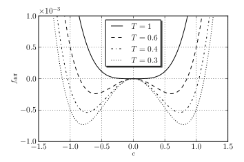
Figure 1: Diffusive free-energy density as a function of $c$ at various temperatures $T$ ($A_{4}=7.31\times 10^{-3}$, $A_{2}=6.62\times 10^{-3}$, $T_{P}=1$).

The further the temperature drops below $T_{P}$, the deeper the energy wells. The existence of two wells is what can lead to regions with layers alternating values of $c$, which is typical of a pearlitic structure. The presence of the term $\nabla c$ in the free-energy accounts for the energy associated with the formation a phase boundaries. In the context of pearlite, it reflects the surface energy associated with the boundaries between cementite and ferrite. Mathematically, it provides a regularising effect when the free-energy is non-convex with respect to $c$. Note that below $T_{P}$ there is no stable local minimum at $c=0$ for the chosen free-energy function.

5.1.2 Displacive part of the free-energy

The displacive part of the free-energy is postulated as follows:

$$f_{\rm disp}=\dfrac{B_{62}}{6}e_{2}^{6}-\dfrac{B_{42}}{4}e_{2}^{4}+\dfrac{B_{22}}{2}\dfrac{T-T_{M}}{T_{M}}e_{2}^{2}+\dfrac{B_{1}}{2}e_{1}\left[{e_{1}-\left({\alpha\left({T-T_{\rm ref}}\right)+x_{1c}c+x_{12}e_{2}^{2}}\right)}\right]\\ +\dfrac{B_{3}}{2}e_{3}^{2}+\frac{\lambda_{e}}{2}\|\nabla e_{2}\|^{2},$$ (28)

where $B_{62}$, $B_{42}$, $B_{22}$, $B_{1}$, $B_{3}$ and $\lambda_{e}$ are positive constants, $T_{M}$ is the non-dimensional temperature below which $f_{\rm disp}$ is non-convex in $e_{2}$, $x_{1c}$ and $x_{12}$ are constant coupling parameters that induce volumetric changes as a consequence of diffusive and displacive phase changes, respectively, and $\alpha>0$ is the thermoelastic coefficient which determines volumetric changes as a consequence of temperature deviations away from a reference temperature $T_{\rm ref}$. The volumetric term in the displacive free-energy is chosen such that the model will coincide with classical thermoelasticity. The displacive contribution to the free-energy as a function of $e_{2}$ at various temperatures is illustrated in Figure 2.

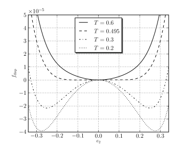
Figure 2: Displacive free-energy density as a function of $e_{2}$ at various temperatures $T$ and $e_{1}=e_{3}=0$ ($B_{62}=3.69$, $B_{42}=1.24\times 10^{-1}$, $B_{22}=4.97\times 10^{-3}$, $T_{M}=0.495$).

Physically, $T_{M}$ is the temperature below which martensite can form. The further the temperature drops below $T_{M}$, the deeper the double-wells in $f_{\rm disp}$ as a function of $e_{2}$. This is what leads to formation of martensite, with spatially alternating values of $e_{2}$ indicating twinning. Analogous to the diffusive contribution to the free-energy, the gradient term $\nabla e_{2}$ accounts for the energy associated with twin boundaries, and provides a regularising effect at temperatures below $T_{M}$. Similar to the diffusive free-energy contribution, below $T_{M}$ there is no stable local minimum at $e_{2}=0$ for the chosen free-energy function.

5.1.3 Thermal part of the free-energy

The thermal part of the free-energy is postulated to be of the classical form

$$f_{\rm therm}=-s_{0}\left({T-T_{\rm ref}}\right)-\frac{c_{v}}{2T_{\rm ref}}\left({T-T_{\rm ref}}\right)^{2},$$ (29)

where $s_{0}$ is the reference entropy density and $c_{v}$ is the heat capacity, both of which are assumed to be positive and constant, and $T_{\rm ref}$ is the aforementioned constant reference temperature.

5.1.4 Phase coupling contribution

Displacive and diffusive phases do not generally co-exists at a given point. To model this, we include in the free-energy a contribution of the form

$$f_{\rm cpl}=x_{2c}c^{2}e_{2}^{2},$$ (30)

where $x_{2c}>0$ is a constant. The task of this term is to penalise energetically concurrent variations away from zero of $e_{2}$ and $c$. That is, it penalises the co-existence of pearlitic ($c\neq 0$) and martensitic phases ($e_{2}\neq 0$).

5.2 Constitutive models as a consequence of the free-energy

The thermodynamic restrictions in Section 4, together with the Helmholtz free-energy defined in this section, provide constitutive models for the stress, the chemical potential and the entropy. We provide now some expansions for these constitutive models in terms of the order parameters for the particular free-energy that we consider.

Introducing the notation $\bar{\boldsymbol{\sigma}}=\partial f/\partial\boldsymbol{\varepsilon}$, for the ‘local’ part of the inviscid stress tensor (see equation (19)), $\bar{\boldsymbol{\sigma}}$ in terms of derivatives of $f$ with respect to the order parameters reads:

$$\bar{\boldsymbol{\sigma}}=\frac{\partial f}{\partial e_{1}}\left({\boldsymbol{e}_{1}\otimes\boldsymbol{e}_{1}+\boldsymbol{e}_{2}\otimes\boldsymbol{e}_{2}}\right)+\frac{\partial f}{\partial e_{2}}\left({\boldsymbol{e}_{1}\otimes\boldsymbol{e}_{1}-\boldsymbol{e}_{2}\otimes\boldsymbol{e}_{2}}\right)+\frac{\partial f}{\partial e_{3}}e_{3}\left({\boldsymbol{e}_{1}\otimes\boldsymbol{e}_{2}+\boldsymbol{e}_{2}\otimes\boldsymbol{e}_{1}}\right),$$ (31)

where $\boldsymbol{e}_{i}$ is a canonical unit basis vector. The divergence of the higher-order stress term $\boldsymbol{\Sigma}=\partial f/\partial\nabla\boldsymbol{\varepsilon}$ (see equation (18)) in terms of the order parameters reads:

$$\nabla\cdot\boldsymbol{\Sigma}=\nabla\cdot\left({\frac{\partial f}{\partial\nabla e_{2}}}\right)\left({\boldsymbol{e}_{1}\otimes\boldsymbol{e}_{1}-\boldsymbol{e}_{2}\otimes\boldsymbol{e}_{2}}\right)=\lambda_{e}\nabla^{2}e_{2}\left({\boldsymbol{e}_{1}\otimes\boldsymbol{e}_{1}-\boldsymbol{e}_{2}\otimes\boldsymbol{e}_{2}}\right).$$ (32)

The chemical potential $\mu$ is of the form (see equation (22)):

$$\mu=\frac{\partial f}{\partial c}-\lambda_{c}\nabla^{2}c,$$ (33)

where $\partial f/\partial c$ is the ‘local’ part of the chemical potential. The time derivative of the entropy density, which will play a role in formulating the heat transport equation, reads:

$$\begin{split}\dot{s}&=-\frac{\partial^{2}f}{\partial T^{2}}\dot{T}-\frac{\partial^{2}f}{\partial T\partial\boldsymbol{\varepsilon}}:\dot{\boldsymbol{\varepsilon}}-\frac{\partial^{2}f}{\partial T\partial\nabla\boldsymbol{\varepsilon}}\vdots\nabla\dot{\boldsymbol{\varepsilon}}-\frac{\partial^{2}f}{\partial T\partial c}\dot{c}-\frac{\partial^{2}f}{\partial T\partial\nabla c}\cdot\nabla\dot{c}\\ &=\frac{c_{v}}{T_{\rm ref}}\dot{T}-\frac{\partial^{2}f}{\partial T\partial e_{1}}\dot{e}_{1}-\frac{\partial^{2}f}{\partial T\partial e_{2}}\dot{e}_{2}-\frac{\partial^{2}f}{\partial T\partial c}\dot{c},\end{split}$$ (34)

where in the last line we have taken into account that temperature does not affect the phase boundary energy.

5.3 Constitutive models for the dissipative terms

Constitutive models for the mass flux, the heat flux and the viscous stress do not follow as a direct consequence of the chosen of the free-energy, but must be chosen such that the restrictions in Section 4 are satisfied. As is usual, the definition of a free-energy does not provide information on the kinetics (rate) of phase transformation processes.

We opt for a viscous stress that depends on the rate of $e_{2}$ only,

$$\boldsymbol{\sigma}_{v}=\nu\dot{e}_{2}\left({\boldsymbol{e}_{1}\otimes\boldsymbol{e}_{1}-\boldsymbol{e}_{2}\otimes\boldsymbol{e}_{2}}\right),$$ (35)

where $\nu\geq 0$, in which case equation (20) is satisfied. The mass flux $\boldsymbol{j}_{c}$ is assumed to be proportional to the chemical potential,

$$\boldsymbol{j}_{c}=-M\nabla\mu,$$ (36)

where $M$ is known as the ‘mobility’. The expression

$$M=M_{0}\exp\left({-\frac{Q}{T}}\right),$$ (37)

where $M_{0}\geq 0$ and $Q\geq 0$ are constants, will be used in the simulations. The thermodynamic restriction in equation (23) is satisfied if $M\geq 0$. For the heat flux, the Fourier model is assumed:

$$\boldsymbol{q}=-k\nabla T,$$ (38)

where $k$ is the thermal conductivity. The thermodynamic restriction in equation (25) is satisfied if $k\geq 0$.

6 Governing initial boundary value problems

A complete set of governing equations for the considered model can now be defined. The model is based on momentum balance, mass balance for the solute phase and an energy balance for heat transport. The primal unknowns to be solved for are the displacement, the solute concentration and the temperature.

The boundary $\partial\Omega$ is assumed to be partitioned into subsets such that $\overline{\partial\Gamma_{h}\cup\partial\Gamma_{g}}=\overline{\partial\Gamma_{q}\cup\partial\Gamma_{T}}=\partial\Omega$ and $\partial\Gamma_{h}\cap\partial\Gamma_{g}=\partial\Gamma_{q}\cap\partial\Gamma_{T}=\emptyset$. The balance of momentum equation follows directly from equation (7). Neglecting differences in mass density between phases, the balance of momentum equation and the associated boundary and initial conditions read:

$$\rho\ddot{\boldsymbol{u}}-\nabla\cdot\boldsymbol{\sigma} =\boldsymbol{b}\quad\ \ {\rm in}\ \Omega\times\left[{0,t_{\rm f}}\right]$$ (39)

$$\boldsymbol{\sigma}\boldsymbol{n} =\boldsymbol{h}_{s}\quad{\rm on}\ \Gamma_{h}\times\left[{0,t_{\rm f}}\right]$$ (40)

$$\boldsymbol{u} =\boldsymbol{g}_{u}\quad{\rm on}\ \Gamma_{g}\times\left[{0,t_{\rm f}}\right]$$ (41)

$$\lambda_{e}\nabla e_{2}\cdot\boldsymbol{n} =0\quad\ \ {\rm on}\ \partial\Omega\times\left[{0,t_{\rm f}}\right]$$ (42)

$$\boldsymbol{u}\left({\boldsymbol{x},0}\right) =\boldsymbol{u}_{0}\quad{\rm on}\ \Omega$$ (43)

$$\dot{\boldsymbol{u}}\left({\boldsymbol{x},0}\right) =\boldsymbol{v}_{0}\quad\,{\rm on}\ \Omega.$$ (44)

The boundary condition $\nabla e_{2}\cdot\boldsymbol{n}=0$ is motivated by the interpretation that the gradient terms provide a nonlocal effect, and in the absence of neighbouring material particles on the boundary no nonlocal work can be done on $\partial\Omega$. This coined the ‘insulation condition’ by Polizzotto (2003).

Inserting the expression for the mass flux in equation (36) into the differential expression of mass conservation (5) leads to an equation governing the transport of the solute. For the form of the free-energy given in Section 5.1 and the definition of $\mu$ in equation (22) in terms of the free-energy, the mass diffusion equation and associated boundary and initial conditions read:

$$\dot{c}-\nabla\cdot M\nabla\left({\frac{\partial f}{\partial c}-\lambda\nabla^{2}c}\right) =0\quad{\rm on}\ \Omega\times\left[{0,t_{\rm f}}\right]$$ (45)

$$M\nabla\left({\frac{\partial f}{\partial c}-\lambda\nabla^{2}c}\right)\cdot\boldsymbol{n} =0\quad{\rm on}\ \partial\Omega\times\left[{0,t_{\rm f}}\right]$$ (46)

$$\lambda_{c}\nabla c\cdot\boldsymbol{n} =0\quad{\rm on}\ \partial\Omega\times\left[{0,t_{\rm f}}\right]$$ (47)

$$c\left({\boldsymbol{x},0}\right) =c_{0}\ \ {\rm on}\ \Omega.$$ (48)

The above equation is known as the Cahn-Hilliard equation. A consequence of the manner in which the surface energy is included in the model is the presence of fourth-order derivatives. The boundary condition in (46) implies that there is no mass flux across $\partial\Omega$ (see (22) and (36)), and (47) is interpreted in the same fashion as the condition on $\nabla e_{2}\cdot\boldsymbol{n}$ in the momentum balance. A more general form of the boundary conditions for the Cahn-Hilliard equation can be found in Wells et al. (2006).

The final governing equation is the energy balance. Using the definition of the Helmholtz free-energy, $\dot{u}$ can be replaced by $\dot{f}+\dot{T}s+T\dot{s}$ in the energy balance (10), yielding

$$\dot{f}+\dot{T}s+T\dot{s}=-\nabla\cdot\boldsymbol{q}+\boldsymbol{\sigma}:\nabla\boldsymbol{v}+(\nabla\cdot\boldsymbol{\Sigma}):\dot{\boldsymbol{\varepsilon}}+\boldsymbol{\Sigma}:\nabla\dot{\boldsymbol{\varepsilon}}\\ +(\nabla\cdot\boldsymbol{\xi})\dot{c}+\boldsymbol{\xi}\cdot\nabla\dot{c}-\mu\nabla\cdot\boldsymbol{j}_{c}-\nabla\mu\cdot\boldsymbol{j}_{c}.$$ (49)

By considering the expansion of $\dot{f}$ in (15) and the constitutive models for $\boldsymbol{\sigma}_{e}$, $\mu$ and $s$ in equations (19), (22) and (24), respectively, the energy balance reduces to

$$T\dot{s}=-\nabla\cdot\boldsymbol{q}+\boldsymbol{\sigma}_{v}:\dot{\boldsymbol{\varepsilon}}-\nabla\mu\cdot\boldsymbol{j}_{c}.$$ (50)

Using the expression of $\dot{s}$ in equation (34), the heat equation, together with suitable boundary and initial conditions reads:

$$\frac{Tc_{v}}{T_{\rm ref}}\dot{T}-T\left({\frac{\partial\boldsymbol{\sigma}}{\partial T}:\dot{\boldsymbol{\varepsilon}}+\frac{\partial\mu}{\partial T}\dot{c}}\right) ‍+\nabla\mu\cdot\boldsymbol{j}_{c} ‍-\boldsymbol{\sigma}_{v}:\dot{\boldsymbol{\varepsilon}}+\nabla\cdot\boldsymbol{q} =0\quad\ \ {\rm on}\ \Omega\times\left[{0,t_{\rm f}}\right]$$ (51)

$$\boldsymbol{q}\cdot\boldsymbol{n} =h_{T}\quad{\rm on}\ \Gamma_{q}\times\left[{0,t_{\rm f}}\right]$$ (52)

$$T =g_{T}\quad{\rm on}\ \Gamma_{T}\times\left[{0,t_{\rm f}}\right]$$ (53)

$$T\left({\boldsymbol{x},0}\right) =T_{0}\quad\,{\rm on}\ \Omega.$$ (54)

The complete model involves the solution of all three coupled equations.

7 Fully-discrete Galerkin formulation

A Galerkin finite element formulation of the governing equations is now developed which will be used in computing numerical examples. A feature of the governing equations is the presence of fourth-order derivatives of the concentration and displacement fields. Ordinarily, this would require finding approximate solutions in a subspace of $H^{2}\left({\Omega}\right)$, but such finite element element spaces are troublesome to construct. We will exploit two different strategies to avoid this difficulty. For the mass diffusion equation it is convenient to adopt a mixed formulation, which is essentially an operating-splitting approach and is not encumbered with the difficulties that plague mixed formulations that result in saddle-point problems. For the momentum balance, mixed schemes are difficult to analyse and in some cases stable schemes may not be known. To circumvent this difficulty, techniques for fourth-order elliptic equations that are inspired by discontinuous Galerkin methods will be used (see Engel et al. (2002); Wells and Dung (2007)). These methods permit the rigorous solution of fourth-order problems using a primal formulation and $H^{1}\left({\Omega}\right)$-conforming finite element spaces.

To formulate a finite element problem, let $\mathcal{T}$ be a triangulation of $\Omega$ into finite element cells such that $\mathcal{T}=\left\{{K}\right\}$. We will work with the usual Lagrange finite element basis

$$V_{k}=\left\{{v\in H^{1}\left({\Omega}\right),v\in P_{k}\left({K}\right)\forall K\in\mathcal{T}}\right\},$$ (55)

where $P_{k}$ denotes the space of Lagrange polynomials of order $k$ on a finite element cell. The numerical formulation that we propose involves solving the following problem: given the data at time $t_{n}$, find $\boldsymbol{u}_{h},c_{h},\tau_{h},T_{h}\in(V_{k_{2}})^{d}\times V_{k_{1}}\times V_{k_{1}}\times V_{k_{1}}$ at time $t_{n+1}$ such that

$$L(\boldsymbol{w},q,r,z;\boldsymbol{u}_{h},c_{h},\tau_{h},T_{h})=0\quad\forall\left({\boldsymbol{w},q,r,z}\right)\in(V_{k_{2}})^{d}\times V_{k_{1}}\times V_{k_{1}}\times V_{k_{1}},$$ (56)

where $k_{2}>1$ and $k_{1}>0$. The functional $L$ is linear in each of $\left({\boldsymbol{v},q,r,w}\right)$ and therefore can be split additively into four contributions:

$$L(\boldsymbol{w},q,r,z;\boldsymbol{u}_{h},c_{h},\tau_{h},T_{h})=L_{u}(\boldsymbol{w};\boldsymbol{u}_{h},c_{h},\tau_{h},T_{h})+L_{c}(q;\boldsymbol{u}_{h},c_{h},\tau_{h},T_{h})\\ +L_{\tau}(r;\boldsymbol{u}_{h},c_{h},\tau_{h},T_{h})+L_{T}(z;\boldsymbol{u}_{h},c_{h},\tau_{h},T_{h}),$$ (57)

where $L_{u}$, $L_{c}$, $L_{\tau}$ and $L_{T}$ will represent the contributions of linear momentum, mass diffusion, the chemical potential and heat transport, respectively. Each of these terms will be defined in this section.

Implicit time integrators will be used for all equations. We believe this to be the only feasible approach owing to the parabolic nature of the mass and heat transport equations, and the presence of fourth-order terms in the momentum balance and mass diffusion equations.

It is particularly convenient to express the problem using the format of equation (56) since we use high-level tools to generate computer code automatically for this problem, and these tools inherit this mathematical expressiveness. Furthermore, the tools perform automatic differentiation (both regular and directional derivatives) so there is no need to compute by hand a linearisation of the problem. The functional $L$ will be the input to the code, and the directional derivative (the linearisation) is computed using automatic differentiation, yielding the Jacobian for use in a Newton solver. This will be expanded upon in the following section.

The subscript ‘$h$’ will be used in this section to denote an approximate quantity, for example $f_{h}=f(\boldsymbol{u}_{h})$, where $\boldsymbol{u}_{h}$ is the approximate displacement field.

7.1 Balance of momentum

Multiplying the balance of momentum equation (39) by a function $\boldsymbol{w}$ and applying integration by parts to various terms,

$$\int_{\Omega}\rho\boldsymbol{w}\cdot\ddot{\boldsymbol{u}}_{h}\,dx+\int_{\Omega}\nabla\boldsymbol{w}:\bar{\boldsymbol{\sigma}}_{h}\,dx+\int_{\Omega}\nabla\boldsymbol{w}:\nabla\cdot\boldsymbol{\Sigma}_{h}\,dx+\int_{\Omega}\nabla\boldsymbol{w}:\boldsymbol{\sigma}_{v,h}\,dx\\ -\int_{\Omega}\boldsymbol{w}\cdot\boldsymbol{b}\,dx-\int_{\partial\Omega}\boldsymbol{w}\cdot\boldsymbol{h}_{s}\,ds=0,$$ (58)

where the decomposition of the stress into ‘local’ and ‘gradient’ contributions has been used, $\boldsymbol{\sigma}_{h,e}=\bar{\boldsymbol{\sigma}}_{h}-\nabla\cdot\boldsymbol{\Sigma}_{h}$, and the Neumann boundary condition $\boldsymbol{\sigma}\boldsymbol{n}=\boldsymbol{h}_{s}$ has been inserted. Addressing now the term involving $\boldsymbol{\Sigma}_{h}$ and considering the precise form of $\boldsymbol{\Sigma}_{h}$ in (32), we have

$$\int_{\Omega}\nabla\boldsymbol{w}:\nabla\cdot\boldsymbol{\Sigma}_{h}\,dx=-\int_{\Omega}\left({w_{1,1}-w_{2,2}}\right)\lambda_{e}\nabla^{2}e_{2,h}\,dx.$$ (59)

This term is problematic since after the application of integration by parts, second-order spatial derivatives of $\boldsymbol{w}$ and $\boldsymbol{u}_{h}$ are present, which classically would require searching for approximate solutions using $H^{2}$-conforming functions, thereby precluding the use of standard Lagrange finite element basis functions. To circumvent this difficulty while still using $H^{1}$-conforming element and without abandoning a primal approach, we introduce integrals over finite element cell facets to impose weak continuity of the normal derivative while preserving consistency and stability, as formulated for the biharmonic equation in Engel et al. (2002) and the Cahn-Hilliard equation in Wells et al. (2006). This then permits the use of standard $H^{1}$-conforming finite element basis functions. The modified variational form, using $\partial f/\partial e_{i}$ in place of $\bar{\boldsymbol{\sigma}}$, reads:

$$L_{u}=\int_{\Omega}\rho\boldsymbol{w}\cdot\ddot{\boldsymbol{u}}_{h,n+1-\alpha_{m}}\,dx+\int_{\Omega}(w_{1,1}+w_{2,2})\frac{\partial f_{h,n+1-\alpha_{f}}}{\partial e_{1}}\,dx+\int_{\Omega}(w_{1,1}-w_{2,2})\frac{\partial f_{h,n+1-\alpha_{f}}}{\partial e_{2}}\,dx\\ +\int_{\Omega}(w_{1,2}+w_{2,1})\frac{\partial f_{h,n+1-\alpha_{f}}}{\partial e_{3}}\,dx+\sum_{K}\int_{K}\nabla\left({w_{1,1}-w_{2,2}}\right)\cdot\lambda_{e}\nabla e_{2,h,n+1-\alpha_{f}}\,dx\\ -\int_{\tilde{\Gamma}}\llbracket{w_{1,1}-w_{2,2}}\rrbracket\cdot\langle{\lambda_{e}\nabla e_{2,h,n+1-\alpha_{f}}}\rangle\,ds-\int_{\tilde{\Gamma}}\langle{\lambda_{e}\nabla\left({w_{1,1}-w_{2,2}}\right)}\rangle\cdot\llbracket{e_{2,h,n+1-\alpha_{f}}}\rrbracket\,ds\\ +\int_{\tilde{\Gamma}}\frac{\eta\lambda_{e}}{h_{K}}\llbracket{w_{1,1}-w_{2,2}}\rrbracket\cdot\llbracket{e_{2,h,n+1-\alpha_{f}}}\rrbracket\,d\Gamma+\int_{\Omega}(w_{1,1}-w_{2,2})\nu e_{2,h,n+1-\alpha_{f}}\,dx\\ -\int_{\Omega}\boldsymbol{w}\cdot\boldsymbol{b}_{n+1-\alpha_{f}}\,dx-\int_{\partial\Omega}\boldsymbol{w}\cdot\boldsymbol{h}_{s,{n+1-\alpha_{f}}}\,ds,$$ (60)

where $\tilde{\Gamma}$ denotes the set of all interior facets, $\llbracket{a}\rrbracket=a_{+}\boldsymbol{n}_{+}+a_{-}\boldsymbol{n}_{-}$ and $\langle{b}\rangle=\left({\boldsymbol{b}_{+}+\boldsymbol{b}_{-}}\right)/2$, ‘$+$’ and ‘$-$’ denote opposite sides of a cell facet, $\eta$ is a dimensionless penalty parameter and $h_{K}$ is a measure of the local element size. The penalty parameter is required for stability of the formulation and is of order one. Time derivatives are dealt with using a generalised-$\alpha$ scheme (see, for example, Chung and Hulbert (1993)). The acceleration, velocity and displacement at the end of a time step are related via

$$\boldsymbol{u}_{n+1} =\boldsymbol{u}_{n}+\Delta t\dot{\boldsymbol{u}}_{n}+\Delta t^{2}\left({\left({\frac{1}{2}-\beta}\right)\ddot{\boldsymbol{u}}_{n}+\beta\ddot{\boldsymbol{u}}_{n+1}}\right),$$ (61)

$$\dot{\boldsymbol{u}}_{n+1} =\dot{\boldsymbol{u}}_{n}+\Delta t\left({\left({1-\gamma}\right)\ddot{\boldsymbol{u}}_{n}+\gamma\ddot{\boldsymbol{u}}_{n+1}}\right),$$ (62)

where $\Delta t=t_{n+1}-t_{n}$, $\beta$ and $\gamma$ are parameters, and mid-point values of primal fields are computed according to

$$y_{n+1-\alpha}=\left({1-\alpha}\right)y_{n+1}+\alpha y_{n}.$$ (63)

where $\alpha$ is a parameter. The parameters $\alpha_{m}$, $\alpha_{f}$, $\gamma$ and $\beta$ determine properties of the time stepping scheme and will be reported with other problem data for the numerical examples in the following section. Nonlinear functions are evaluated at a mid-point, for example

$$f_{n+\alpha}=f(T_{n+\alpha},e_{i,n+\alpha},\nabla e_{2,n+\alpha},c_{n+\alpha},\nabla c_{n+\alpha}).$$ (64)

The discontinuous Galerkin-type approach is consistent for $k>1$, and analysis of the biharmonic equation has shown that the method is stable for sufficiently large $\alpha$ (typically $\alpha$ is of order $1$). It has been proven that the method converges in the $L^{2}$ for the biharmonic equation at a rate of $k+1$ for $k>2$ (Engel et al., 2002) and at a rate of $k$ for $k=2$ (Wells and Dung, 2007).

7.2 Mixed form of the Cahn-Hilliard equation

For the Cahn-Hilliard equation we adopt an operator splitting approach to deal with the fourth-order spatial derivative and split equation (45) into two second-order equations:

$$\dot{c}-\nabla\cdot M\nabla\tau =0,$$ (65)

$$\tau-\frac{\partial f}{\partial c}+\lambda_{c}\nabla^{2}c =0,$$ (66)

where $c$ and $\tau$ are the independent unknowns that will be solved for. If the above problem is solved exactly, then $\tau$ and $\mu$ will coincide (see equation (22)). It will be important to distinguish between $\tau$ and $\mu$ when finding approximate solutions. Note that through $\partial f/\partial c$ there is a dependency on the strain and the temperature.

Casting the above set of equations into a weak form, using the Crank-Nicolson method for the time derivative, and applying the boundary conditions from equations (47) and (46), the functionals $L_{c}$ and $L_{\tau}$ read:

$$L_{c} =\int_{\Omega}q\frac{c_{h,n+1}-c_{h,n}}{\Delta t}\,dx+\int_{\Omega}\nabla q\cdot M\nabla\tau_{h,n+1/2}\,dx,$$ (67)

$$L_{\mu} =\int_{\Omega}r\tau_{h,n+1}\,dx-\int_{\Omega}r\frac{\partial f_{h,n+1}}{\partial c}\,dx-\int_{\Omega}\nabla r\cdot\lambda_{c}\nabla c_{h,n+1}\,dx.$$ (68)

This operator splitting approach to the Cahn-Hilliard equation was presented and analysed by Elliott et al. (1989), and for the form of the free-energy and mobility considered by Elliott et al. (1989) it was shown to be stable. A discontinuous Galerkin type approach, similar to that used for the momentum equation, can also be used to solve the Cahn-Hilliard equation in its primal form (Wells et al., 2006).

7.3 Heat transport equation

The heat equation (51) can be cast into a weak form via the usual process. Using the Crank-Nicolson method to deal with time derivatives, the functional $L_{T}$ reads:

$$L_{T}=\int_{\Omega}z\frac{T_{h,n+1/2}}{T_{\rm ref}}c_{v}\frac{T_{h,n+1}-T_{h,n}}{\Delta t}\,dx\\ -\int_{\Omega}zT_{h,n+1/2}\left({\frac{\partial\boldsymbol{\sigma}_{e,h,{n+1/2}}}{\partial T}:\frac{\boldsymbol{\varepsilon}_{h,n+1}-\boldsymbol{\varepsilon}_{h,n}}{\Delta t}+\frac{\partial\mu_{n+1/2}}{\partial T}\frac{c_{h,n+1}-c_{h,n}}{\Delta t}}\right)\,dx\\ ‍+\int_{\Omega}z\left({\nabla\tau_{h,n+1/2}\cdot\boldsymbol{j}_{n+1/2}-\boldsymbol{\sigma}_{v,{n+1/2}}:\frac{\boldsymbol{\varepsilon}_{n+1}-\boldsymbol{\varepsilon}_{n}}{\Delta t}}\right)\,dx\\ -\int_{\Omega}\nabla z\cdot\boldsymbol{q}_{h,n+1/2}\,dx-\int_{\Gamma_{q}}zh_{q,_{n+1/2}}\,ds.$$ (69)

Taking into account details of the constitutive models,

$$L_{T}=\int_{\Omega}z\left({\frac{T_{h,n+1/2}}{T_{\rm ref}}c_{v}\frac{T_{h,n+1}-T_{h,n}}{\Delta t}\,dx-\sum_{i=1}^{3}T_{h,n+1/2}\left({\frac{\partial^{2}f}{\partial e_{i}\partial T}\frac{e_{i,h,n+1}-e_{i,h,n}}{\Delta t}}\right)}\right)\,dx\\ -\int_{\Omega}z\left({T_{h,n+1/2}\frac{\partial^{2}f}{\partial c\partial T}\frac{c_{i,h,n+1}-c_{i,h,n}}{\Delta t}+\nabla\tau_{h,n+1/2}\cdot M_{h}\nabla\tau_{h,n+1/2}}\right)\,dx\\ ‍-\int_{\Omega}z\nu e_{2,h,n+1/2}\frac{e_{2,h,n+1}-e_{2,h,n}}{\Delta t}\,dx+\int_{\Omega}\nabla z\cdot k_{T}\nabla T_{h,n+1/2}\,dx-\int_{\Gamma_{q}}zh_{q,_{n+1/2}}\,ds.$$ (70)

8 Numerical examples

A number of numerical examples are now presented to demonstrate that the model can qualitatively capture classical processes observed in the heat treatment of steels. It is not the intention to consider realistic material parameters at this stage. The determination of physical parameters, and computing with these, is a substantial undertaking and is the subject of ongoing work.

The model includes a number of coupled processes, which permits considerable freedom in how transformations are induced, and a variety of parameters play a role in the development of microstructure. The presented examples involve varying the heat flux across the boundary of the domain for a fixed set of model parameters. For the parameters appearing in the free-energy, the following values are used: $A_{4}=7.3\times 10^{-3}$; $A_{2}=6.6\times 10^{-3}$; $T_{P}=1$; $\lambda_{c}=1\times 10^{-7}$; $B_{62}=0.3$; $B_{42}=3.1\times 10^{-3}$; $B_{22}=2.5\times 10^{-3}$; $B_{3}=5\times 10^{-2}$; $\lambda_{e}=1\times 10^{-8}$; $T_{M}=0.495$; $\alpha=1\times 10^{-2}$; $x_{1c}=5\times 10^{-3}$; $x_{12}=1\times 10^{-1}$; $c_{T}=3.5\times 10^{-8}$; and $x_{2c}=8\times 10^{-2}$. For model parameters that do not appear in the free-energy, the following values are used: $\rho=5\times 10^{-7}$; $\nu=5\times 10^{-8}$; $k_{T}=2\times 10^{-2}$; $M_{0}=1\times 10^{4}$; and $Q=5$. The adopted time stepping parameters are $\rho_{\infty}=0.7$; $\alpha_{m}=(2\rho_{\infty}-1)/(\rho_{\infty}+1)$; $\alpha_{f}=\rho_{\infty}/(\rho_{\infty}+1)$; $\beta=(1-\alpha_{m}+\alpha_{f})^{2}/4$; and $\gamma=1/2-\alpha_{m}+\alpha_{f}$. The time stepping parameters are chosen such that the momentum balance scheme is second-order accurate and strongly stable (at least for linear problems). The mobility $M$ as a function of temperature for the adopted parameters is plotted in Figure 3. There is considerable scope for a extensive computational studies into the impact of various parameters on different microstructural processes.

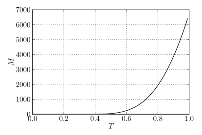
Figure 3: Mobility as a function of temperature.

All simulations are performed on a unit domain $\Omega=(0,1)\times(0,1)$ using triangular finite element cells in a regular diagonal pattern and with 128 vertices in each direction. For the displacement field, $\Gamma_{g}={(x,0)\cup(0,y)\in\partial\Omega}$ with $\boldsymbol{u}=\boldsymbol{0}$ on $\Gamma_{g}$ and $\boldsymbol{h}_{s}=\boldsymbol{0}$ on $\Gamma_{h}=\partial\Omega\backslash\Gamma_{g}$. With this boundary condition, any effect of a displacement constraint on microstructure evolution will be evident. The heat flux across $\partial\Omega$, which we denoted by $h_{q}$, is set proportional to the difference between the temperature $T$ on the boundary and a prescribed ‘external’ temperature $T_{\rm ext}$:

$$h_{q}=-\delta\left({T-T_{\rm ext}}\right),$$ (71)

where $\delta\geq 0$ is a parameter. The larger the value of $\delta$, the more rapid the cooling. Other boundary conditions were defined in Section 6. The impact of the cooling rate on the microstructure development will be examined by varying $\delta$ and $T_{\rm ext}$. The initial conditions for the displacement and concentration are fields that are perturbed randomly about zero. In the case of the concentration field, $c_{0}\in\left[{-10^{-4},10^{-4}}\right]$ is a random number with a uniform distribution, and for the initial displacement, $\boldsymbol{u}_{0}\in\left[{-10^{-4}h_{K},10^{-4}h_{K}}\right]^{2}$ is a random vector with a uniform distribution and $h_{K}$ is a measure of the finite element cell size. The dependency on the cell size is introduced so that the magnitude of the initial strains is roughly equal on different meshes. In all simulations $T_{\rm ref}=T_{0}=1.2$.

Quadratic Lagrange functions are used for the displacement field and linear Lagrange functions are used for all other fields ($k_{2}=2$ and $k_{1}=1$ in equation (56)). A fully-coupled solution strategy is used and a Newton-Krylov method is employed to solve the nonlinear equations in each time step. For the stabilising penalty term, $\eta=8$. The problem-specific parts of the computer code used to perform the simulations have been generated automatically from a high-level description that resembles closely the notation used in this work by using a number of tools from the FEniCS Project (Logg and Wells, 2010; Ølgaard and Wells, 2010; Ølgaard et al., 2008). The complete computer code used to perform all simulations reported in this work consists of one file only and is freely available under a GNU public license for both scrutiny and use (Wells and Maraldi, 2011).

8.1 Rapid boundary cooling to $T_{\rm ext}=0.1$

We first consider rapid cooling from an initial uniform temperature of $T=1.2$, at which temperature austenite is the stable phase, down to $T_{\rm ext}=0.1$, which is well-below the martensitic transition temperature of $T_{M}=0.495$. At $T=0.1$, the mobility of the diffusive phase is negligible, hence for this rapid cooling case the formation of a diffusive phase is not anticipated; the resulting structure will therefore be martensite. To simulate rapid cooling, the boundary heat flux parameter $\delta=5\times 10^{-2}$ is used. For this case, simulations were performed with an initial time step of $\Delta t=1\times 10^{-4}$, which was increased to $\Delta t=2\times 10^{-3}$ at $t=0.266$. The computed order parameter $e_{2}$ at various times during the cooling process is shown in Figure 4. The diffusive variable $c$ (not shown) is very close to zero everywhere in the domain. The rapid formation of fine martensite twins can be observed in Figure 4. Note that the martensite twins are slightly less developed at the left-hand and lower edges of the domain, due to the constraint $\boldsymbol{u}=\boldsymbol{0}$, which inhibits lattice distortion on these constrained boundaries. This is also what induces the bottom left-hand corner to top right-hand corner orientation of the twins, rather than at 90^∘ to this orientation.

$t=0.01$	$t=0.015$	$t=0.025$	$t=0.3$

Figure 4: Contours of the displacive order parameter $e_{2}$ for the rapid cooling case to $T_{\rm ext}=0.1$. The approximate range of temperatures in the domain at the snapshots are: at $t=0.01$, $T\approx 0.27-0.61$; at $t=0.015$, $T\approx 0.17-0.31$; at $t=0.025$, $T\approx 0.1$; and at $t=0.3$, $T\approx 0.1$.

8.2 Boundary cooling to $T_{\rm ext}=0.3$ at different rates

We now consider a less deep quench to $T_{\rm ext}=0.3$, which is still below the martensitic transition temperature, with the same boundary heat flux parameter of $\delta=5\times 10^{-2}$. At $T=0.3$, the mobility of the diffusive phase is still negligible. For this case, simulations were performed with a time step of $\Delta t=2.5\times 10^{-4}$. The order parameter $e_{2}$ at various times during the cooling process is shown in Figure 5. For this case, the field $c$ (not shown) is close to zero throughout the simulation, despite the diffusive phase being energetically favourable over the displacive phase, because diffusive processes are unable to develop due to the brief length of time over which the temperature, and hence the mobility, is sufficiently high. As with the $T_{\rm ext}=0.1$ case, martensite forms quickly, although it is now slightly coarser in the early stages. On a slightly longer time scale, there is some limited twin boundary motion as part of a minimal coarsening process. Such coarsening is not observed at lower temperatures, and can be attributed to the different balance between bulk and surface energy (in the model, the surface energy is unaffected by temperature while the bulk energy is). Noteworthy is that the microstructure that forms in this case is more affected by the displacement constraint on the two sides of the domain. This can be explained by the smaller thermodynamic force driving the $e_{2}$ patterning compared to the $T_{\rm ext}=0.1$ case.

For this cooling case, the temperature contours are shown at two snapshots in Figure 6. In the absence of thermal coupling effects, the temperature contours would be symmetric about the $x$- and $y$-axes. Figure 6 shows a subtle breaking of symmetry. In particular, at $t=0.02$ an alignment of contours with the direction of the martensite twins can be detected. The presented simulations are driven by large changes in the boundary heat flux, which makes it difficult to detect local temperature changes due to phase changes since these are relatively small, but also with possibly high gradients that are smoothed rapidly by conduction. The heat capacity plays a large role in temperature changes since it determines the change in temperature associated with a given energy release during a transformation.

$t=0.0175$	$t=0.02$	$t=0.05$	$t=0.5$

Figure 5: Contours of the displacive order parameter $e_{2}$ for the rapid cooling case ($\delta=5\times 10^{-2}$) to $T_{\rm ext}=0.3$. The approximate range of temperatures in the domain at the snapshots are: at $t=0.0175$, $T\approx 0.35-0.45$; at $t=0.02$, $T\approx 0.32-0.41$; at $t=0.05$, $T\approx 0.3$; and at $t=0.5$, $T\approx 0.3$.

$t=0.0175$	$t=0.02$

Figure 6: Temperature contours for the rapid cooling case ($\delta=5\times 10^{-2}$) to $T_{\rm ext}=0.3$. Thermal coupling effects lead to the subtle breaking of symmetry in the temperature contours. Symmetry is restored at later times via heat conduction.

An intermediate cooling rate case with $\delta=1.5\times 10^{-3}$ and a time step of $\Delta t=2\times 10^{-3}$ is now considered. For this case, the order parameters $e_{2}$ and $c$ are shown in Figure 7 at a number if time steps. At this cooling rate, the impact of non-isothermal effects are clear. There is sufficient time for a diffusive phase to develop in three of the corners. The formation of a diffusive phase in the corners is accelerated by the combination thermoelastic effects and the boundary constraints and the temperature changes. Upon cooling, regions of volumetric straining with opposite signs develop in three of the corners which, due to the $x_{1c}\neq 0$, encourages diffusion of $c$. However, before a diffusive phase can form in the entire domain, the temperature drops to a level at which the mobility is too low for diffusion to continue, and martensite twins form in the regions in which the diffusive phase has not yet developed. For $t>1$, the phase configuration is essentially stable and no further changes could be detected. Figure 8 shows the temperature contours for this case at four time instants. Initially a bias can be detected with the warmest region running between the two regions with the most developed diffusive phases (at $t=0.25$). As time progresses, a subtle alignment of the temperature contours can be detected. At long times, the temperature field is smoothed by conduction, but at $t=0.2$ very subtle temperature variations can be detected, with the temperature contours aligned with the martensite twins. This can be attributed to very slow twin coarsening effects.

$e_{2}$
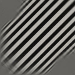
$c$
	$t=0.25$	$t=0.4$	$t=0.5$	$t=2$

Figure 7: The displacive order parameter $e_{2}$ and the diffusive order parameter $c$ for the moderate cooling rate case to $T_{\rm ext}=0.3$. The approximate temperature in the domain at the snapshots is: at $t=0.25$, $T\approx 0.62$; at $t=0.4$, $T\approx 0.45$; at $t=0.5$, $T\approx 0.38$; and at $t=2$, $T\approx 0.3$.

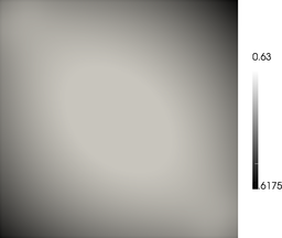
$t=0.25$	$t=0.4$
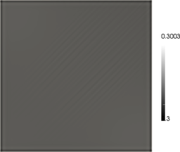
$t=0.5$	$t=2$

Figure 8: Temperature contours for the moderate cooling rate case to $T_{\rm ext}=0.3$. Variations of the temperature contours away from a symmetric pattern are attributable to thermal coupling effects. At $t=2$, very subtle temperature contours aligned with the martensite twins can be detected.

Even slower cooling rate cases are now considered, from which the impact of the cooling rate on the structure of the diffusive phase can be observed. For $\delta=1\times 10^{-3}$ and $\Delta t=2\times 10^{-3}$, the evolution of the diffusive phase is shown in Figure 9.

$t=0.3$	$t=0.4$	$t=0.6$	$t=4$

Figure 9: Contours of the diffusive order parameter $c$ for the slow cooling case ($\delta=1\times 10^{-3}$) to $T_{\rm ext}=0.3$. The approximate temperature in the domain at the snapshots is: at $t=0.3$, $T\approx 0.72$; at $t=0.4$, $T\approx 0.76$; at $t=0.6$, $T\approx 0.66$; and at $t=4$, $T\approx 0.3$.

At this cooling rate, a reasonably fine microstructure develops, with considerable domain boundary coherence. That is, the lamella near the boundaries are aligned with the boundary. Between $t=0.3$ and $t=0.4$ the temperature in the domain increases due to the energy released during the transformation, and the time is insufficient for conduction to transport the heat across the boundary of the domain. The microstructural features change if the cooling rate is slowed further, as shown in Figure 10, where $\delta=1\times 10^{-4}$ and $\Delta t=1\times 10^{-2}$.

$t=1.75$	$t=2.5$	$t=4$	$t=8$

Figure 10: Contours of the diffusive order parameter $c$ for the very slow cooling case ($\delta=1\times 10^{-4}$) to $T_{\rm ext}=0.3$. The approximate temperature in the domain at the snapshots is: at $t=1.75$, $T\approx 0.91$; at $t=2.5$, $T\approx 0.89$; at $t=4$, $T\approx 0.8$; and at $t=8$, $T\approx 0.6$.

The microstructure is clearly coarser, and the boundary coherence is reduced. Beyond $t=8$, further microstructural changes could not be perceived.

8.3 Rapid boundary cooling to $T_{\rm ext}=0.4$

The domain is now cooled to $T=0.4$ with $\delta=5\times 10^{-2}$. The time step was changed during the simulation, and ranged between $\Delta t=2.5\times 10^{-4}$ and $\Delta t=5\times 10^{-2}$. At $T=0.4$, diffusive processes are very slow, but not yet negligible. For this case, the computed contours of $e_{2}$ and $c$ are presented in Figure 11.

$e_{2}$
$c$
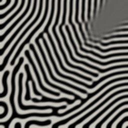
	$t=0.1$	$t=6$	$t=9$	$t=15$	$t=24$

Figure 11: The displacive order parameter $e_{2}$ and the diffusive order parameter $c$ for the rapid cooling case to $T_{\rm ext}=0.4$. At all snapshots, the temperature in the domain is approximately $0.4$.

It is clear that martensite twins form initially. The thermodynamic driving force for the development of a diffusive phase is greater than for the displacive phase, although it is inhibited by the low mobility, but eventually diffusive process can be detected and the diffusive phase slowly replaces the displacive phase. At this external temperature, the structure of the diffusive phase is quite fine.

An extremely challenging aspect of computations at this temperature is reconciling the dramatic time scale differences for the different processes, especially during the latter stages. The diffusive phase develops very slowly, but the evolution of the diffusive phase can induce sporadic changes in the martensitic phase. Using a time step that is suitable for diffusive processes can lead to a loss of solution stability when sporadic displacive changes take place. There is considerable scope for developing efficient, robust and accurate methods for spanning the large difference in time scales.

8.4 Rapid boundary cooling to $T_{\rm ext}=0.45$

The final example is rapid cooling with $\delta=5\times 10^{-2}$ to $T_{\rm ext}=0.45$. The time step was changed during the simulation, and ranged between $\Delta t=5\times 10^{-4}$ and $\Delta t=2\times 10^{-1}$. Snapshots of the order parameters $e_{2}$ and $c$ are presented in Figure 12.

$e_{2}$
$c$
	$t=0.04$	$t=0.1$	$t=0.4$	$t=2$	$t=7$

Figure 12: The displacive order parameter $e_{2}$ and the diffusive order parameter $c$ for the rapid cooling case ($\delta=5\times 10^{-2}$) to $T_{\rm ext}=0.45$. At all snapshots, the temperature in the domain is approximately $0.45$.

As expected, martensite develops quickly. Interestingly, the domain then undergoes a rearrangement between $t=0.1$ and $t=0.4$, in which $e_{2}$ goes from an alternating pattern to a value close to zero in the bottom left-hand region of the domain. It is likely that this is due to the boundary constraint resisting deformation, and the driving force for the square-to-rectangular transition being too small to overcome this constraint. In the top right-hand triangle, $e_{2}$ is approximately constant at $t=0.4$. At $T=0.45$, the driving force behind the development of the alternating $e_{2}$ pattern is relatively weak, whereas the energy associated with phase boundaries does not have a direct temperature dependency. The system undergoes another change between $t=0.4$ and $t=2$, with the sign of $e_{2}$ in the upper right-hand region changing. On a longer time scale, diffusive processes develop, first in the region where $e_{2}\approx 0$ and then progressing in into the region where $e_{2}$ is not equal to zero, eventually replacing the martensite phase. Noteworthy is the lack of structure in the diffusive phase in the bottom left-hand triangular region, and the more coherent lamella structure in the upper right-hand region.

As for the previous example, computing solutions to this problem robustly and on a reasonable computational time scale is extremely challenging.

9 Conclusions

A phase field model that can simulate both diffusive and displacive phase transitions has been presented. The model is developed in a formal thermodynamic setting, with free-energy expressions associated with distinct microstructural processes, the postulation of an energy balance and demonstration that the classical entropy inequality is satisfied. Various couplings terms introduce dependencies between different processes. The model includes both bulk energy and phase boundary energy, which impacts on the fineness of the computed microstructures. Surface energies have been introduced via higher-order spatial gradients of the relevant order parameters, and this demands special care in the formulation of the thermodynamic balance laws. To satisfy the classical point-wise form of the entropy inequality, non-standard stress-like terms have been introduced to the energy balance equation. These non-local terms are related to phase boundary surface energy, and represent the work done by particles that neighbour an arbitrary subdomain.

The differential equations that follow from the fundamental balance laws involve the displacement field, the solute concentration and the temperature field, with significant couplings between all equations. The presence of surface energies in the model leads to a momentum balance and mass balance (diffusion) equations that involve fourth-order spatial derivatives. The presence of the higher-order derivatives is problematic when developing a Galerkin finite element method for solving the problem. To counter this, a sophisticated Galerkin method has been formulated for the problem that imposes the classically required solution regularity in a weak sense. The computer model has been generated for a large part automatically from a high-level specification, and is published as supporting material.

It has been demonstrated through numerical simulations that the proposed model can capture qualitatively a variety of observed phenomena, including the formation of martensite twins, the development of pearlitic structures and pearlite replacing martensite when a specimen is held at a sufficiently high temperature for an extended period. Phase transitions have been triggered via control of heat flux across the boundary, but transformations can also be induced by mechanical loading. The application of the model with physically determined parameters requires further investigation. Such an investigation will also necessitate further development of numerical solution strategies to enable simulations on large domains and appropriate time scales to be performed both accurately and within a tolerable simulation time.

References

- Alt and Pawlow (1992) Alt, H. W., Pawlow, I., 1992. A mathematical model of dynamics of non-isothermal phase separation. Physica D: Nonlinear Phenomena 59, 389–416.
- Ball (2004) Ball, J. M., 2004. Mathematical models of martensitic microstructure. Materials Science and Engineering A 278, 61–69.
- Ball and James (1987) Ball, J. M., James, R. D., 1987. Fine phase mixtures as minimizers of energy. Archive for Rational Mechanics and Analysis 100 (1), 13–52.
- Barsch and Krumhansl (1984) Barsch, G. R., Krumhansl, J. A., 1984. Twin boundaries in ferroelastic media without interface dislocations. Physical Review Letters 53 (11), 1069–1072.
- Bhadeshia (1987) Bhadeshia, H. K. D. H., 1987. Worked examples in the geometry of crystals. The Institute of Metals, London.
- Bhattacharya (1991) Bhattacharya, K. V., 1991. Wedge-like microstructure in martensites. Acta Metallurgica et Materialia 39, 2431–2444.
- Bouville and Ahluwalia (2006) Bouville, M., Ahluwalia, R., 2006. Interplay between diffusive and displacive phase transformations: Time-temperature-transformation diagrams and microstructures. Physical Review Letters 97 (5), 055701.
- Bouville and Ahluwalia (2007) Bouville, M., Ahluwalia, R., 2007. Effect of lattice-mismatch-induced strains on coupled diffusive and displacive phase transformations. Physical Review B 75 (5), 054110.
- Bowles and McKenzie (1954) Bowles, J. S., McKenzie, J. K., 1954. The crystallography of martensite transformations I. Acta Metallurgica 2 (1), 129–137.
- Cahn and Hilliard (1958) Cahn, J. W., Hilliard, J. E., 1958. Free energy of a nonuniform system. I. Interfacial free energy. The Journal of Chemical Physics 28, 258–267.
- Chung and Hulbert (1993) Chung, J., Hulbert, G. M., 1993. A time integration algorithm for structural dynamics with improved numerical dissipation: The generalized- method. Journal of Applied Mechanics 60 (2), 371–375.
- Elliott et al. (1989) Elliott, C. M., French, D. A., Milner, F. A., 1989. A 2nd-order splitting method for the Cahn-Hilliard equation. Numerische Mathematiek 54 (5), 575–590.
- Engel et al. (2002) Engel, G., Garikipati, K., Hughes, T. J. R., Larson, M. G., Taylor, R. L., 2002. Continuous/discontinuous finite element approximations of fourth-order elliptic problems in structural and continuum mechanics with applications to thin beams and plates, and strain gradient elasticity. Computer Methods in Applied Mechanics and Engineering 191 (34), 3669–3750.
- Falk (1980) Falk, F., 1980. Model free energy, mechanics, and thermodynamics of shape memory alloys. Acta Metallurgica 28 (12), 1773–1780.
- Gurtin (1965) Gurtin, M. E., 1965. Thermodynamics and the possibility of spatial interaction in elastic materials. Archive for Rational Mechanics and Analysis 19 (5), 339–352.
- Gurtin (1996) Gurtin, M. E., 1996. Generalized Ginzburg-Landau and Cahn-Hilliard equations based on a microforce balance. Physica D 92, 178–192.
- Harrison et al. (2004) Harrison, R. J., Redfern, S. A. T., Buckley, A., Salje, E. K. H., 2004. Application of real-time, stroboscopic x-ray diffraction with dynamical mechanical analysis to characterize the motion of ferroelastic domain walls. Journal of Applied Physics 95 (4), 1706–1717.
- Jacobs (1985) Jacobs, A. E., 1985. Solitons of the square-rectangular martensitic transformation. Physical Review B 31 (9), 5984–5989.
- Kohn (1991) Kohn, R. V., 1991. Relaxation of a double-well energy. Continuum Mechanics and Thermodynamics 3 (3), 193–236.
- Logg and Wells (2010) Logg, A., Wells, G. N., 2010. DOLFIN: Automated finite element computing. ACM Transactions on Mathematical Software 37 (2), 20:1–20:28.
-
Maraldi et al. (2010)
Maraldi, M., Molari, L., Grandi, D., 2010. A thermodynamical model for
concurrent diffusive and displacive phase transitions.
URL http://arxiv.org/abs/1012.2994 - Ølgaard et al. (2008) Ølgaard, K. B., Logg, A., Wells, G. N., 2008. Automated code generation for discontinuous Galerkin methods. SIAM Journal on Scientific Computing 31 (2), 849–864.
- Ølgaard and Wells (2010) Ølgaard, K. B., Wells, G. N., 2010. Optimisations for quadrature representations of finite element tensors through automated code generation. ACM Transactions on Mathematical Software 37 (1), 8:1–8:23.
- Onuki (1999) Onuki, A., 1999. Pretransitional effects at structural phase transitions. Journal of the Physical Society of Japan 68 (1), 5–8.
- Polizzotto (2003) Polizzotto, C., 2003. Gradient elasticity and nonstandard boundary conditions. International Journal of Solids and Structures 40 (26), 7399–7423.
- Shenoy et al. (1999) Shenoy, S. R., Lookman, T., Saxena, A., Bishop, A. R., 1999. Martensitic textures: multiscale consequences of elastic compatibility. Physical Review B 60 (18), R12 537–R12 541.
- Wang and Khachaturyan (1997) Wang, Y., Khachaturyan, A. G., 1997. Three-dimensional field model and computer modeling of martensitic transformations. Acta Materialia 45 (2), 759–773.
- Wang et al. (1993) Wang, Y., Wang, H., Chen, L. Q., Khachaturyan, A. G., 1993. Shape evolution of a coherent tetragonal precipitate in partially stabilized cubic ZrO2: A computer simulation. Journal of the American Ceramic Society 76 (12), 3029–3033.
- Wayman (1990) Wayman, C. M., 1990. The growth of martensite since E. C. Bain (1924) – some milestones. Materials Science Forum 56–58, 1–32.
- Wechsler et al. (1953) Wechsler, M. S., Lieberman, D. S., Read, T. A., 1953. On the theory of the formation of martensite. Journal of Metals 197, 1503–1515.
- Wells and Dung (2007) Wells, G. N., Dung, N. T., 2007. A discontinuous Galerkin formulation for Kirchhoff plates. Computer Methods in Applied Mechanics and Engineering 196 (35–36), 3370–3380.
- Wells et al. (2006) Wells, G. N., Kuhl, E., Garikipati, K., 2006. A discontinuous Galerkin formulation for the Cahn-Hilliard equation. Journal of Computational Physics 218 (2), 860–877.
-
Wells and Maraldi (2011)
Wells, G. N., Maraldi, M., 2011. Supporting material.
URL http://www.dspace.cam.ac.uk/handle/1810/236975