Xingbo Yuan1, Yang Hao1 and Ya-Dong Yang1,2 1Institute of Particle Physics, Huazhong Normal University, Wuhan, Hubei 430079, P. R. China
2Key Laboratory of Quark & Lepton Physics, Ministry of Education, Huazhong Normal University,
Wuhan, Hubei, 430079, P. R. China
Abstract
Observation of top quark flavor changing neutral process at the LHC would be the signal of physics beyond the Standard Model. If anomalous coupling exists, it will affect the precisely measured . In this paper, we study the effects of a dimension 5 anomalous operator in decay to derive constraints on its possible strength. It is found that, for real anomalous coupling , the constraints correspond to the upper bounds (for ) and (for ), respectively, which are about the same order as the discovery potential of ATLAS () and slightly lower than that of CMS () with integrated luminosity operating at TeV.
I Introduction
In the Standard Model (SM), top quark lifetime is dominated by the process, and its flavor changing neutral current (FCNC) processes are extremely suppressed by GIM mechanism. It is known that the SM predicts very tiny top FCNC branching ratio , less than gadi , which would be inaccessible at the CERN Large Hadron Collider(LHC). In the literature gadicp ; Beneke , however, a number of interesting questions have been intrigued by the large top quark mass which is close to the scale of electroweak symmetry breaking. For example, one may raise the question whether new physics (NP) beyond the SM could manifest itself in nonstandard couplings of top quark which would show up as anomalies in the top quark productions and decays.
At present, the direct constraints on are still very weak. For its radiative decay, the available experimental bounds are from ZEUS ZEUS and
from CDF CDF at C.L., respectively. These constraints will be improved greatly by the large top quark sample to be available at the LHC, which is expected to produce top quark pairs and another few million single top quarks per year at low luminosity (/year). Both ATLAS
ATLAS and CMS CMS have got analyses ready for hunting out top quark FCNC processes as powerful probes for NP. With data, it is expected that both ATLAS and CMS could observe decays if their branching ratios are enhanced to by anomalous top quark couplings ATLAS ; CMS . However, if the top quark anomalous couplings present, they will affect some precisely measured qualities with virtual top quark contribution. Inversely, these qualities can also restrict the possible number of top quark FCNC decay signals at the LHC. The precisely measured inclusive decay is one of the well known sensitive probes for extensions of the SM, especially the NPs which alter the strength of FCNCs top . Thus, when performing the study of the possible strength of decays at the LHC, one should take into account the constraints from wtb ; Fox .
In this paper, we will study the contribution of anomalous operators to the
branching ratio and derive constraints on its strength. In the next section, after a brief discussion of a set of model-independent dimension 5 effective operators relevant to decay, we calculate the effects of operator in decay, which result in a modification to . In Sec. III we present our numerical results of the constraints on its strength and the corresponding upper limits on branching ratio of decays. Finally, conclusions are made in Sec. IV. Calculation details are presented in Appendix A, and input parameters are collected in Appendix B.
II Top quark anomalous couplings and their effects in decay
Without resorting to the detailed flavor structure of a specific NP model, the Lagrangian describing the top quark anomalous couplings can be written in a model independent way with dimension 5 operators lag1
(1)
where is the complex coupling of its corresponding operator, is the weak angle, and is the Gell-Mann matrix. is the possible new physics scale, which is unknown but may be much larger than the electroweak scale. There are also Lagrangian describing the top quark anomalous interactions with dimension 4 and 6 operators, and the dimension 4 and 5 terms can be traced back to dimension 6 operators wyler ; list . In fact top quark anomalous interactions can be generally described by the gauge-invariant effective Lagrangian with dimension 6 operators in a form without redundant operators and parameters Fox ; Saavedra . A recent full list of dimension 6 operators could be found in Ref. SM6 . But for on-shell gauge bosons, the Lagrangian in Eq. (1) works and is commonly employed in high energy phenomenology analysis Beneke ; ATLAS ; Li .
It is understood that the Dirac matrix connects left-handed fields to right-handed
fields, the transition will involve two independent operators
and ,
where the mass factors must appear whenever a chirality flip or
occurs. Due to the mass hierarchy , the effect of can be neglected unless is enhanced to be comparable to by unknown mechanism.
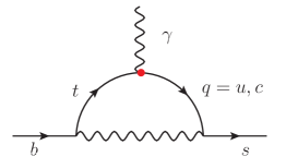
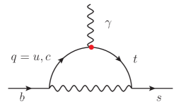
The anomalous coupling affects decays through the two Feynman diagrams depicted in Figs. 1 and 1. It is interesting to note that the CKM factors in Fig. 1 and Fig. 1 are and , respectively. Since for , the contribution of Fig. 1 would be much stronger than that of Fig. 1. Furthermore, given the strengths of and comparable, the contribution of Fig. 1 to is still dominated by because of . Hence we will only consider Fig. 1 with anomalous
coupling.
From the Feynman diagram of Fig. 1, it is easy to observe that the large CKM factor makes very sensitive to the strength of anomalous coupling.
The calculation of Fig. 1 can be carried out straightforwardly. The calculation details are presented in Appendix A, and the final result reads
(3)
Usually term can be neglected, and the function is calculated to be
(4)
with . Now we are ready to incorporate the NP contribution into its SM counterpart for decay.
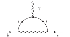
Figure 1: Feynman diagrams for . (a) and (b) are the penguin diagrams with the anomalous
couplings. (c) Sample LO penguin diagram in the SM.
In the SM, it is known that decay is governed by the effective Hamiltonian at scale
Buras1
(5)
where are the Wilsion coefficients, are the effective four quark operators and
(6)
For calculating , instead of the original Wision coefficients , it is convenient to
use the so called “effective coefficients” Buras94
(7)
where and
(8)
(9)
To the leading order approximation, the is proportional to
Buras .
In terms of the operator basis in Eq. (5), the contribution of the anomalous couplings
in Eq. (3) would result in the deviation of
From this equation, one can see that the NP contribution is suppressed by a factor of but enhanced by .
Since NP contribution does not bring about any new operator, the renormalization group evolution of from to scale is just the same as the SM one in Eq. (7). For GeV, GeV, and TeV, we have
(12)
In principle, will receive corrections from anomalous couplings
in Eq. (1) which will cause a deviation to . However, as shown by Eq. (12), the coefficient of is about one order larger than of .
Given the relative strength of to
at level, will be shifted by only few percentage. For simplifying the numerical analysis, we would neglect the contribution of the anomalous couplings. We also find that the operator
contributes to
only through the term as shown by Eq. (3) and Eq. (7).
Combined with the previous remarks on this operator, the effects of
could be safely neglected.
III Numerical results and discussions
The current average of experimental results of by Heavy Flavor Average Group is HFAG
(13)
On the theoretical side, the NLO calculation has been completed Misiak ; Buras , and gives
(14)
The recent estimation at NNLO Misiak1 gives
,
which is about lower than the experimental average in Eq. (13). Thus the experimental measurement of is in good agreement with the SM predictions with roughly errors on each side. The agreement would provide strong constraints on the top quark anomalous interactions beyond the SM wtb ; Fox .
The decay amplitude of has been calculated up to NLO Li . For a consistent treatment of the constraints from and decays, we use the NLO formulas in Ref. Misiak to calculate . The experimental inputs and main formulas are collected in Appendix B.
For numerical analysis, we will use the notation
and set TeV.
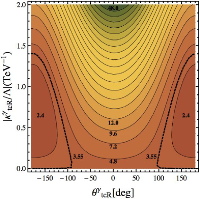
Figure 2: The contour-plot describes the dependence of
on
and . The dashed lines correspond to the experimental center
value of .
At first, we analyze the dependence of on the new physics parameters
and , which is shown in Fig. 2.
From the figure, one can find that the contribution of anomalous
coupling is constructive to the SM one for ,
thus is very sensitive to .
However, when ,
the sensitivity of to becomes weak.
For , the contribution of anomalous coupling is destructive to the SM one and there are two separated possible strengths for .
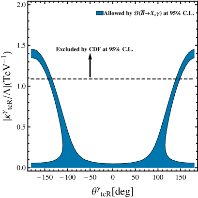
Figure 3: The C.L. upper bounds on anomalous coupling as a function of .
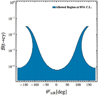
The shadowed region is allowed by and the dash-line is the CDF CDF upper limit.Figure 4: as a function of . The shadowed region is allowed by the combined constraints of
and CDF searching at 95% C.L.
The allowed region for the parameters and under the constraints from at C.L. is shown in Fig. 3. The corresponding C.L. upper bound on is shown in Fig. 4.
Now we turn to discuss the our numerical results. From Eq. (12), the explicit relation
between the SM and the coupling contributions is
(15)
Obviously, when , the interference between them is constructive,
and it turns to be destructive when . Thus the features of these constraints shown in Figs. 3 and 4 for different
are
(i)
the bound on is very strong for
. For , as shown in Fig. 3, we obtain the most restrictive upper bound , which implies ;
(ii)
the bound on is rather weak for around
. For such a case, is destructive to the SM contribution as shown by
Eq. (15), so, the allowed strength for the anomalous coupling is much larger than the one for real . When and , is almost imaginary since
.
Then the restriction on is provided by the CDF search for CDF ;
(iii)
as shown in Fig. 3, when , there are two solutions for .
The larger one (S2 column in Table 1) corresponds to the situation that the sign of is flipped. However, it has been excluded by
the CDF upper bound of CDF .
The another solution (S1 column in Table 1) will result in the upper limit .
Taking and as benchmarks, we summarize
our numerical constraints on and their corresponding upper limits on in Table 1. From the table, we can find that our indirect bound on real is much stronger than the CDF direct bound. The corresponding upper limits on are about the same order as the ATLAS sensitivity ATLAS and CMS sensitivity
CMS with an integrated luminosity of of the LHC operating at TeV ATLAS .
Table 1: The 95% C.L. constraints on the anomalous coupling by and for some specific values.
In this paper, starting with model independent dimension five anomalous operators, we have studied
their contributions to . It is noted that
the transition will involve two independent operators
and . The first operator will produce a left-handed photon in decay, while the second one will produce a right-handed photon.
It is found that is sensitive to the first operator, but not to the second one.
For real , the constraint on the presence of
is very strong, which corresponds to the indirect upper limits
(for positive ) and
(for negative ), respectively.
These upper limits for are close to the discovery sensitivities of ATLAS ATLAS and slightly lower than that of CMS CMS with integrated luminosity operating
at TeV.
For nearly imaginary , the constraints are rather weak since in the SM is
a real number. If were found to be of the order of
at the LHC in the future, it would imply the weak phase of
to be around . However, such a coupling might be ruled out by the other observable in B meson decays xqli .
In summary, we have studied the interesting interplay between the precise measurement of decay at B factories and the possible decay at the LHC. For real anomalous coupling, it is shown that has been restricted to be blow at C.L. by decay, which is already two order lower than the direct upper bound from CDF CDF . The result also implies that one may need data sample much larger than to hunt out signals at the LHC.
ACKNOWLEDGMENTS
The work is supported by National Natural Science Foundation under contract
Nos.11075059 and 10735080. We thank Xinqiang Li for many helpful discussions and cross-checking calculations.
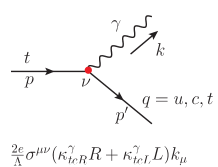
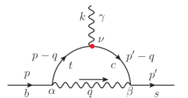
Figure 5: (a) the Feynman rules of interactions in the Lagrangian of Eq. 1. (b) penguin diagram contribution to with top quark anomalous interactions.
Appendix A The calculation of
Using the Feynman rules in Fig 5, the amplitude of penguin diagram in Fig 5 can be written as,
(1)
(2)
(3)
with and . By Dirac algebra
(4)
the terms with in vanishes and N becomes
(5)
Thus, there is no divergence in . After integrating out in the and using on-shell condition, can be written in the following form,
The experimental inputs are collected in Table. 2, in which the CKM factors are derived from the Wolfenstein parameters A, , and .
References
(1)
G. Eilam, J.L. Hewett and A.Soni,
Phys. Rev. D44, 1473(1991), Erratum-ibid D59, 039901(1999).
(2)
D. Atwood, S. Bar-Shalom, G. Eilam and A. Soni,
Phys. Rept. 347, 1(2001), arXiv: hep-ph/0006032.
(3)
There are many papers on top quark rare decays.
For a review, we refer to M. Beneke et al.,
arXiv:hep-ph/0003033 and references therein.
(4)
S. Chekanov et al. [ZEUS Collaboration],
Phys. Lett. B 559, 153 (2003)
[arXiv:hep-ex/0302010].
(5)
F. Abe et al. [CDF Collaboration],
Phys. Rev. Lett. 80, 2525 (1998).
(6)
J. Carvalho et al. [ATLAS Collaboration],
Eur. Phys. J. C 52, 999 (2007)
[arXiv:0712.1127 [hep-ex]].
F. Veloso, et al. CERN-THESIS-2008-106.
(7)
L. Benucci and A. Kyriakis,
Nucl. Phys. Proc. Suppl. 177-178, 258 (2008).
(8)
M. Antonelli et al., Phys. Rept.494, 197(2010),
arXiv:0907.5386 [hep-ph].
(9)
B. Grzadkowski and M. Misiak, Phys. Rev. D 78, 077501(2008).
(10)
P. J. Fox, Z. Ligeti, M. Papucci, G. Perez, and M. D. Schwartz,
Phys. Rev. D 78, 054008(2008).
(11)
W. Hollik, J. I. Illana, S. Rigolin, C. Schappacher and D. Stockinger,
Nucl. Phys. B 551, 3 (1999)
[Erratum-ibid. B 557, 407 (1999)]
[arXiv:hep-ph/9812298].
(12)
W. Buchmuller and D. Wyler,
Nucl. Phys. B 268, 621 (1986).
(13)
K. Hagiwara, S. Ishihara, R. Szalapski and D. Zeppenfeld,
Phys. Rev. D 48, 2182 (1993).
G. J. Gounaris, F. M. Renard and C. Verzegnassi,
Phys. Rev. D 52, 451 (1995)
[arXiv:hep-ph/9501362].
G. J. Gounaris, F. M. Renard and N. D. Vlachos,
Nucl. Phys. B 459, 51 (1996)
[arXiv:hep-ph/9509316].
K. Whisnant, J. M. Yang, B. L. Young and X. Zhang,
Phys. Rev. D 56, 467 (1997)
[arXiv:hep-ph/9702305].
J. M. Yang and B. L. Young,
Phys. Rev. D 56, 5907 (1997)
[arXiv:hep-ph/9703463].
(14)
J. A. Aguilar-Saavedra,
Nucl. Phys. B 812, 181 (2009)
[arXiv:0811.3842 [hep-ph]].
(15)
B. Grzadkowski, M. Iskrzyński, M. Misiak, and J. Rosiek, arXiv: 1008.4884 [hep-ph].
(16)
J. J. Zhang, C. S. Li, J. Gao, H. Zhang, Z. Li, C. P. Yuan and T. C. Yuan,
Phys. Rev. Lett. 102, 072001 (2009)
[arXiv:0810.3889 [hep-ph]].
J. Drobnak, S. Fajfer, and Jernej F. Kamenik, Phys.Rev.Lett. 104, 252001(2010)
[arXiv:1004.0620 [hep-ph]]
(17)
A. J. Buras,
arXiv:hep-ph/9806471.
G. Buchalla, A. J. Buras. and M.E. Lautenbacher, Rev. Mod. Phys. 68, 1125(1996).
(18)
A.J. Buras, M. Misiak, M. Münz, and S. Pokorski, Nucl. Phys. 424, 374(1994)
(19)
E. Barberio et al. [Heavy Flavor Averaging Group],
arXiv:0808.1297 [hep-ex].
(20)
P. Gambino and M. Misiak,
Nucl. Phys. B 611, 338 (2001)
[arXiv:hep-ph/0104034].
(21)
A. J. Buras, A. Czarnecki, M. Misiak and J. Urban,
Nucl. Phys. B 631, 219 (2002)
[arXiv:hep-ph/0203135].
(22)
M. Misiak et al.,
Phys. Rev. Lett. 98, 022002 (2007)
[arXiv:hep-ph/0609232].
(23)
C. W. Bauer, Z. Ligeti, M. Luke, A. V. Manohar and M. Trott,
Phys. Rev. D 70, 094017 (2004)
[arXiv:hep-ph/0408002].
(24)
C. S. Li, R. J. Oakes and T. C. Yuan,
Phys. Rev. D 43, 3759 (1991).
(25)
K. Nakamura et al. (Particle Data Group), J. Phys. G 37, 075021 (2010)
Cut-off date for this update was January 15, 2010.
(26)
J. Charles et al. [CKMfitter Group],
Eur. Phys. J. C 41, 1 (2005)
[arXiv:hep-ph/0406184].
(27)
A. H. Hoang and A. V. Manohar,
Phys. Lett. B 633, 526 (2006)
[arXiv:hep-ph/0509195].
(28)
B. Aubert et al. [BABAR Collaboration],
Phys. Rev. D 81, 032003 (2010)
[arXiv:0908.0415 [hep-ex]].
(29)
P. Gambino and U. Haisch,
JHEP 0110, 020 (2001)
[arXiv:hep-ph/0109058].