Coxeter Groups and
Asynchronous Cellular Automata

Abstract

The dynamics group of an asynchronous cellular automaton (ACA) relates properties of its long term dynamics to the structure of Coxeter groups. The key mathematical feature connecting these diverse fields is involutions. Group-theoretic results in the latter domain may lead to insight about the dynamics in the former, and vice-versa. In this article, we highlight some central themes and common structures, and discuss novel approaches to some open and open-ended problems. We introduce the state automaton of an ACA, and show how the root automaton of a Coxeter group is essentially part of the state automaton of a related ACA.

1 Introduction

An asynchronous cellular automaton (ACA) is defined in the same manner as a classical cellular automaton (CA) in all aspects except the evaluation mechanism. As the name suggests, the maps associated to the vertices (or nodes) are applied synchronously for a CA, and asynchronously for an ACA. In general, there are many ways that one can apply maps asynchronously. For example, one may select a vertex at random according to some probability distribution, apply the corresponding map, and repeat this procedure. Alternatively, one may select a fixed permutation over the vertices and apply the maps in the sequence specified by this permutation. This permutation evaluation process would correspond to increasing the time by one unit, and would be applied repeatedly to generate the system dynamics. An important aspect of having a fixed permutation update sequence is that one obtains a dynamical system. This is not necessarily the case in the more general situation, such as when the individual states are updated at random.

The analysis of CAs and ACAs does not have the support that the study of ODEs has from established fields such as analysis and differential geometry. As such, a key goal of CA/ACA research is to make connections to existing mathematical theory. We will consider the class of $\pi$-independent ACAs – those whose periodic points (as a set) are independent of the permutation update sequence. While this may seem to be a rather exotic property, we have shown that roughly 40% of the elementary CA rules give rise to $\pi$-independent ACAs [8]. Given a $\pi$-independent ACA, one can define its dynamics group. This permutation group on the set of periodic points is a quotient of a Coxeter group, and it captures the possible long-term dynamics that one can generate by suitable choices of update sequence. Its structure can answer questions about the existence and non-existence of periodic orbits of given sizes.

In this paper, we will revisit the notions of Coxeter systems and sequential dynamical systems (SDSs). An SDS is a generalization of an ACA (assuming a fixed update sequence) where the underlying graph is arbitrary, and is not limited to being a regular lattice or circle (i.e., a one-dimensional torus). We will show how the word problem for Coxeter groups is related to functional equivalence of SDS maps. This forms the basis for our next result, on how conjugation of Coxeter elements corresponds to cycle equivalence of SDS maps, and additionally, how this extends from conjugacy classes to spectral classes. After defining dynamics groups and showing how they arise as quotients of Coxeter groups, we show how key features of mathematical objects in both the fields of SDSs and Coxeter groups are encoded by finite (or infinite) state automata. We illustrate this by explicit examples, and then close with a table summarizing these connections.

2 Background

A Coxeter system is a pair $(W,S)$ consisting of a group $W$ generated by a set $S=\{s_{1},\dots,s_{n}\}$ of involutions given by the following presentation

$$W=\langle s_{1},\dots,s_{n}\mid s_{i}^{2}=1,\;\;(s_{i}s_{j})^{m(s_{i},s_{j})}=1\rangle\,,$$

where $m(s_{i},s_{j})\geq 2$ for $i\neq j$. Let $S^{*}$ be the free monoid over $S$, and for each integer $m\geq 0$ and distinct generators $s,t\in S$, define

$$\langle s,t\rangle_{m}=\underbrace{stst\cdots}_{m}\in S^{*}\,.$$

The relation $\langle s,t\rangle_{m(s,t)}=\langle t,s\rangle_{m(s,t)}$ is called a braid relation, and is additionally called a short braid relation if $m(s,t)=2$. Note that $s$ and $t$ commute if and only if $m(s,t)=2$. A Coxeter system can be described uniquely by its Coxeter graph $\Gamma$, which has vertex set $V=\{1,\dots,n\}$ and an edge $\{i,j\}$ for each non-commuting pair of generators $\{s_{i},s_{j}\}$, with edge label $m(s_{i},s_{j})$.

Switching to ACAs and SDSs, let $\Gamma$ be an undirected graph (called the base graph or dependency graph) with vertex set $V=\{1,\dots,n\}$. We equip each vertex $i$ with a state $x_{i}\in K$ where $K$ is a set called the state space, and a vertex function $f_{i}$ that maps (or updates) $x_{i}(t)$ to $x_{i}(t+1)$ based on the states of its neighbors (itself included). Unless explicitly stated otherwise, we will assume that $K=\mathbb{F}_{2}=\{0,1\}$, which is the most commonly used state space in cellular automata research. If the vertex functions are applied asynchronously, it is convenient to encode $f_{i}$ as a $\Gamma$-local function $F_{i}\colon K^{n}\to K^{n}$ defined by

$$F_{i}(x_{1},\dots,x_{n})=(x_{1},\dots,x_{i-1},f_{i}(x_{1},\dots,x_{n}),x_{i+1},\dots,x_{n})\;.$$

If $f_{i}$ does not depend on all $n$ states, it may be convenient to omit the fictitious variables. Given a sequence of local functions and a word $w=w_{1}w_{2}\dots w_{m}\in V^{*}$ called the update sequence, the SDS map $F_{w}$ is the composition of the local functions in the order prescribed by $w$, i.e.,

$$F_{w}\colon K^{n}\longrightarrow K^{n}\,,\qquad F_{w}=F_{w_{m}}\circ F_{w_{m-1}}\circ\cdots\circ F_{w_{2}}\circ F_{w_{1}}\,.$$

SDSs represent a generalization of ACAs, which are usually defined over a regular grid, such as $\mathbb{Z}$ or $\mathbb{Z}_{n}$. The following example illustrates some SDS concepts – see [14] for a more complete treatment.

Example 1

We take $\Gamma=\mathrm{Circ}_{4}$ as base graph (see Figure 1) and use $K=\{0,1\}$ as the state space. Also, we take all vertex functions to be Boolean $\mathrm{nor}$-functions given by $\mathrm{nor}\colon K^{3}\to K$ where $\mathrm{nor}(x,y,z)$ equals $1$ if $x=y=z=0$ and $0$ otherwise. In this case we have, for example, $F_{1}(x_{1},x_{2},x_{3},x_{4})=(\mathrm{nor}(x_{4},x_{1},x_{2}),x_{2},x_{3},x_{4})$. Using the update sequence $\pi=1234$, we obtain

$$F_{1}(0,0,0,0) =(1,0,0,0)$$

$$F_{2}\circ F_{1}(0,0,0,0) =(1,0,0,0)$$

$$F_{3}\circ F_{2}\circ F_{1}(0,0,0,0) =(1,0,1,0)$$

$$F_{4}\circ F_{3}\circ F_{2}\circ F_{1}(0,0,0,0) =(1,0,1,0)\;,$$

and thus $F_{\pi}(0,0,0,0)=(1,0,1,0)$. The phase space of the map $F_{\pi}$ is the directed graph containing all global state transitions and is shown in Figure 1.

    

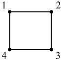
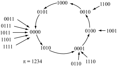
Figure 1: The base graph $\Gamma=\mathrm{Circ}_{4}$ and the phase space of $F_{\pi}$ from Example 1.

3 The word problem

A fundamental question given any finitely presented group $\langle S\mid R\rangle$, is when do two words

$$w=w_{1}w_{2}\cdots w_{m}\,,\quad\mbox{and}\quad w^{\prime}=w^{\prime}_{1}w^{\prime}_{2}\cdots w^{\prime}_{k}$$

in $S^{*}$ yield the same group element? This is the word problem, and it is in general undecidable. However, there are many classes of groups for which the word problem is solvable. A classic result in Coxeter groups, known as Matsumoto’s theorem [5, Theorem 1.2.2], says that any two reduced expressions for the same element differ by braid relations. Matsumoto’s theorem provides an algorithmic solution to the word problem for Coxeter groups.

There is an analog of the word problem for SDSs. Specifically, given two update sequences $w,w^{\prime}\in V^{*}$, when are the corresponding SDS maps

$$F_{w}=F_{w_{m}}\circ F_{w_{m-1}}\circ\cdots\circ F_{w_{2}}\circ F_{w_{1}}\,,\qquad F_{w^{\prime}}=F_{w^{\prime}_{k}}\circ F_{w^{\prime}_{k-1}}\circ\cdots\circ F_{w^{\prime}_{2}}\circ F_{w^{\prime}_{1}}\,$$

equal as functions, or equivalently, when do they have identical phase spaces? This is clearly solvable because there are only finitely many functions $\mathbb{F}_{2}^{n}\to\mathbb{F}_{2}^{n}$. However, it would be desirable to solve this problem algorithmically for general SDSs, without resorting to checking the image of all $2^{n}$ global states.

4 Equivalences on Dynamics and Acyclic Orientations

In this section, we show how topological conjugation of SDS maps corresponds to conjugation of elements in a Coxeter group, and how this connection leads to a coarser equivalence relation when the graph $\Gamma$ has non-trivial symmetries. Acyclic orientations are mathematically convenient to capture several types of equivalences on permutation SDS maps, as well as on Coxeter elements in Coxeter groups. A Coxeter element is the product of the generators of $S$ in some order. Every Coxeter element defines a partial ordering on $S$, which we can represent by an acyclic orientation of $\Gamma$. Specifically, for a Coxeter element $c$, define the orientation $(\Gamma,c)$ so that edge $\{i,j\}$ is oriented $(i,j)$ if $s_{i}$ appears before $s_{j}$ in $c$. It is easy to show that this is well-defined, and that it defines a bijection between the set $\operatorname{Acyc}(\Gamma)$ of acyclic orientations of $\Gamma$ and the set $\operatorname{C}(W)$ of Coxeter elements of $W$.

Next, consider conjugating a Coxeter element $c=s_{x_{1}}\cdots s_{x_{n}}$ by the initial letter $s=s_{x_{1}}$, which results in a cyclic shift of the word:

$$scs=s_{x_{1}}(s_{x_{1}}s_{x_{2}}\cdots s_{x_{n}})s_{x_{1}}=s_{x_{2}}s_{x_{3}}\cdots s_{x_{n}}s_{x_{1}}\,.$$

The corresponding acyclic orientations $(\Gamma,c)$ and $(\Gamma,scs)$ differ by converting the source vertex of $(\Gamma,c)$ into a sink. This source-to-sink conversion generates an equivalence relation $\sim_{\kappa}$ on $\operatorname{Acyc}(\Gamma)$, and it was recently proven (see [4]) that $(\Gamma,c)\sim_{\kappa}(\Gamma,c^{\prime})$ if and only if $c$ and $c^{\prime}$ are conjugate. (Note that the “if” direction is obvious; the “only if” direction is difficult).

Turning to SDSs, let $S_{n}\subset V^{*}$ be the set of words where each vertex appears precisely once, which we may identify with the permutations of $V$. Each permutation $\pi\in S_{n}$ defines a partial ordering on $V$, and there is a natural map from $\operatorname{Acyc}(\Gamma)$ to the set of permutation SDS maps ($\pi$ is mapped to $F_{\pi}$). Two finite dynamical systems $\phi,\psi\colon K^{n}\to K^{n}$ are said to be cycle equivalent if for some bijection $h\colon K^{n}\to K^{n}$ we have $\psi|_{\operatorname{Per}(\psi)}\circ h=h\circ\phi|_{\operatorname{Per}(\phi)}\;,$ where $\operatorname{Per}(\phi)$ denotes the set of periodic states of $\phi$. The following result provides the connection between $\kappa$-equivalence of acyclic orientations and cycle equivalence of permutation SDS maps.

Theorem 4.1 ([12])

If $(\Gamma,\pi)\sim_{\kappa}(\Gamma,\sigma)$, then $F_{\pi}$ and $F_{\sigma}$ are cycle equivalent.

If the automorphism group $\operatorname{Aut}(\Gamma)$ is non-trivial, we can say even more. The group $\operatorname{Aut}(\Gamma)$ acts on $\operatorname{Aut}(\Gamma)/\!\!\sim_{\kappa}$ by $\gamma\cdot[(\Gamma,\pi)]=[(\Gamma,\gamma\pi)]$, which gives rise to the equivalence relation $\sim_{\bar{\kappa}}$ on $\operatorname{Aut}(\Gamma)/\!\!\sim_{\kappa}$. This coarser equivalence relation also has an interpretation in the settings of both Coxeter groups and SDSs.

If $(W,S)$ is a Coxeter system with $|S|=n$, let $\mathcal{V}$ be an $n$-dimensional real vector space with basis $\{\vec{\alpha}_{1},\dots,\vec{\alpha}_{n}\}$. Put a symmetric bilinear form $B$ on $\mathcal{V}$, defined by $B(\vec{\alpha}_{i},\vec{\alpha}_{j})=-\cos\bigl{(}\pi/m(s_{i},s_{j})\bigr{)}$. The group $W$ acts on $\mathcal{V}$ by

$$s_{i}\colon\vec{v}\mapsto\vec{v}-2B(\vec{v},\vec{\alpha}_{i})\vec{\alpha}_{i}\,,$$ (1)

and the set of elements $\Phi=\{w\vec{\alpha}_{i}\mid w\in W\,,i=1,\dots,n\}$ are called roots. This action is faithful and preserves the bilinear form $B$. Geometrically, the root $s_{i}\vec{v}$ is the reflection of $\vec{v}$ across the hyperplane $\vec{\alpha}_{i}^{\perp}$, and so there is a representation $\rho\colon W\to\operatorname{GL}(\mathcal{V})$, defined on the generators by

$$\rho\colon s_{i}\longmapsto\big{(}\vec{v}\stackrel{{\scriptstyle F_{i}}}{{\mapsto}}\vec{v}-2B(\vec{v},\vec{\alpha}_{i})\vec{\alpha}_{i}\big{)}\,,$$ (2)

called the standard geometric representation of $W$ (see [1, 7]). This allows us to view elements in $W$ as matrices, and hence we can speak of the characteristic polynomial of any given $w\in W$.

Now, if $(\Gamma,c)$ and $(\Gamma,c^{\prime})$ differ by some $\gamma\in\operatorname{Aut}(\Gamma)$, then $\rho(c)$ and $\rho(c^{\prime})$ are similar as linear transformations. Specifically, they are conjugate in $\operatorname{GL}(\mathcal{V})$ by the permutation matrix $P_{\gamma}$ of $\gamma$. In this case, we say that $c$ and $c^{\prime}$ have the same spectral class, because $\rho(c)$ and $\rho(c^{\prime})$ have the same multiset of eigenvalues. Clearly, this is a weaker condition than conjugacy, and so all Coxeter elements in the same $\bar{\kappa}$-equivalence class have the same spectral class.

Similarly, in the context of SDSs, if $(\Gamma,\pi)\sim_{\bar{\kappa}}(\Gamma,\sigma)$, then the SDS maps $F_{\pi}$ and $F_{\sigma}$ are cycle equivalent, due to the following argument. If $\gamma\in\operatorname{Aut}(\Gamma)$, then the permutations $\pi$ and $\gamma\pi$ give topologically conjugate SDS maps, $F_{\pi}$ and $F_{\gamma\pi}$. Strictly speaking, this requires the maps $f_{i}$ to be $\operatorname{Aut}(\Gamma)$-invariant (see [12]), a condition which is frequently satisfied in practice, such as when all vertices of the same degree share the same symmetric function (e.g., logical AND, OR, Majority, Parity, threshold functions, etc.). Since topologically conjugate maps are cycle equivalent, our statement follows.

It is worth mentioning the role of the Tutte polynomial here [15]. The Tutte polynomial of a graph $\Gamma$ is a 2-variable polynomial $T_{\Gamma}(x,y)$ that satisfies a recurrence under edge deletion and contraction, and plays a central role in graph theory. Many graph counting problems are simply the evaluation of the Tutte polynomial at some $(x_{0},y_{0})\in\mathbb{Z}\times\mathbb{Z}$. For example, $|\operatorname{Acyc}(\Gamma)|=T_{\Gamma}(2,0)$ and $|\operatorname{Acyc}(\Gamma)/\!\!\sim_{\kappa}\!\!|=T_{\Gamma}(1,0)$. Thus, $T_{\Gamma}(2,0)$ counts the number of Coxeter elements in the Coxeter group with Coxeter graph $\Gamma$, and it bounds the number of permutation SDS maps in an SDS with dependency graph $\Gamma$. This bound is known to be sharp for certain classes of functions [14]. Similarly, $T_{\Gamma}(1,0)$ counts the number of conjugacy classes of Coxeter elements (see [4, 10]), and it bounds the number of cycle equivalence classes of SDS maps (see [12]).

5 Groups

A sequence $F=(F_{1},\dots,F_{n})$ of local functions is $\pi$-independent if $\operatorname{Per}(F_{\pi})=\operatorname{Per}(F_{\sigma})$ for all $\pi,\sigma\in S_{n}$. Note that this is an equality of sets; we do not assume anything about the organization of the respective periodic points into periodic orbits. In this case, each $F_{i}$ permutes the periodic points, and these permutations generate the dynamics group of $F$, denoted $\mathcal{DG}(F)$. Let $F_{i}^{*}$ denote the restriction of $F_{i}$ to $\operatorname{Per}(F_{\pi})$. Because $F_{i}$ only changes the $i^{\rm th}$ coordinate of a state, and since we assume that $K=\mathbb{F}_{2}$, $F_{i}^{*}\circ F_{i}^{*}$ is the identity function on $\operatorname{Per}(F_{\pi})$. If we define $m_{ij}:=|F^{*}_{i}\circ F^{*}_{j}|$, then there is a surjection

$$\langle s_{1},\dots,s_{n}\mid s_{i}^{2}=1,\;(s_{i}s_{j})^{m_{ij}}=1\rangle\longrightarrow\mathcal{DG}(F)\,,$$ (3)

showing that dynamics groups are quotients of Coxeter groups. The particular homomorphism is determined by adding relations to the presentation of the Coxeter group, and these relations arise because the state space is $\mathbb{F}_{2}$. Thus, dynamics groups are in a sense “reflection groups over $\mathbb{F}_{2}$.” An open-ended research problem is to give an efficient presentation of the dynamics groups of an SDS based on the functions, i.e., to determine these extra relations.

When the base graph $\Gamma$ of an SDS is the circular graph $\mathbb{Z}_{n}$, and the local functions are all identical, the resulting SDS is an elementary ACA. Each local function $F_{i}$ takes $\{x_{i-1},x_{i},x_{i+1}\}$ as input, and is completely described by the following rule table

$$\begin{array}[]{c||c|c|c|c|c|c|c|c}x_{i-1}x_{i}x_{i+1}&111&110&101&100&011&010&001&000\\ \hline\cr f_{i}(x_{i-1},x_{i},x_{i+1})&a_{7}&a_{6}&a_{5}&a_{4}&a_{3}&a_{2}&a_{1}&a_{0}\end{array}$$

Clearly, there are $2^{2^{3}}=256$ such choices of functions, which can be indexed by $k=\sum a_{i}2^{i}\in\{0,\dots,255\}$. The corresponding sequence of local functions is denoted $\operatorname{ECA}_{k}$. In [8], it was shown that $\operatorname{ECA}_{k}$ is $\pi$-independent for precisely 104 values of $k$. Moreover, this holds for all $n>3$. The dynamics groups of these 104 rules were classified in [11]. Among some of the interesting groups were $\mathcal{DG}(\operatorname{ECA}_{60})=\operatorname{SL}_{n}(\mathbb{F}_{2})$ and $\mathcal{DG}(\operatorname{ECA}_{k})=\mathbb{Z}_{2}^{n}$ for $k\in\{28,29,51\}$. Moreover, other dynamics groups were found computationally to be either the symmetric or alternating groups, with the size depending on the $n^{\rm th}$ Fibonacci or Lucas number, leading to a few conjectures.

6 The root automaton

The dynamics of all possible SDSs given a sequence of $\Gamma$-local functions $F=(F_{1},\dots,F_{n})$ can be encoded by the state automaton of the sequence. This is a directed graph $\Phi$ with vertex set $K^{n}$ – the set of global system states, and directed edges $(x,F_{i}(x))$ for each $x\in K^{n}$ and each $i\in V$. Label such an edge with the index $i$ corresponding to its vertex function; see Figure 2 for an example.

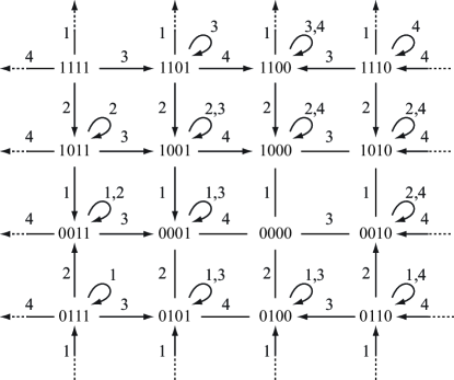
Figure 2: The state automaton $\Phi$ for the SDS in Example 1. Horizontal/vertical dashed lines and arrows indicate horizontal/vertical wrap-around, and arrowheads are omitted from the bidirectional edges for clarity.

The image of a state $x\in K^{n}$ under an SDS map $F_{\pi}$, where $\pi=\pi_{1}\pi_{2}\cdots\pi_{n}$, is represented on the state automaton by a path in $\Phi$. Specifically, start at vertex $x$ and traverse the path

$$x\,,\quad F_{\pi_{1}}(x)\,,\quad F_{\pi_{2}}F_{\pi_{1}}(x)\,,\quad\dots\quad,\,F_{\pi_{n}}\!\cdots F_{\pi_{2}}F_{\pi_{1}}(x)=F_{\pi}(x)\,.$$

The phase space of $F_{\pi}$ can be easily derived from the state automaton – it is the graph with vertex set $K^{n}$ and an edge $(x,y)$ for every directed path from a state $x$ to $y$ that traverses a path of edges labeled $\pi_{1},\pi_{2},\dots,\pi_{n}$. Note that if $F$ is $\pi$-independent, then $\mathcal{DG}(F)$ acts on $\operatorname{Per}(F)$. In this case, all of the edges within $\operatorname{Per}(F)$ are bidirectional, and so we may view them as undirected.

This is the SDS analog of the action of $W$ on $\Phi\subset\mathcal{V}$, as described in (1). Since $\mathcal{V}$ is any $n$-dimensional vector space, we can identify it with $\mathbb{R}^{n}$, and assume that the basis elements are $\vec{\alpha}_{i}=\vec{e}_{i}$, the standard unit normal vectors. This associates roots with vectors in $\mathbb{R}^{n}$, and we partially order $\Phi$ by $\leq$ componentwise ($\vec{z}\preceq\vec{z}^{\prime}$ iff $z_{i}\leq z^{\prime}_{i}$ for each $i$) to get the root poset. It is well-known that for every root, all non-zero entries have the same sign, thus we have a notion of positive and negative roots, and the root poset has a positive side $\Phi^{+}$ and a negative side, $\Phi^{-}$, with $\Phi=\Phi^{+}\cup\Phi^{-}$. The image of $s_{i}$ under the geometric representation from (2) is a linear map $F_{i}\colon\mathbb{R}^{n}\to\mathbb{R}^{n}$, where

$$F_{i}\colon(z_{1},\dots,z_{n})\longmapsto(z_{1},\dots,z_{i-1},z_{i}+\sum_{j=1}^{n}2\cos(\pi/m_{i,j})z_{j},z_{i+1},\dots,z_{n})\;.$$ (4)

To summarize, $F_{i}$ changes the $i^{\rm th}$ entry of a vector by flipping its sign and then adding each neighboring state $z_{j}$ weighted by $2\cos(\pi/m_{ij})$.

In 1993, Brink and Howlett proved that Coxeter groups are automatic [2], and soon after, H. Eriksson developed the root automaton [3]. The root automaton has vertex set $\Phi$ and edge set $\{(\vec{z},s_{i}\vec{z})\mid\vec{z}\in\Phi,\,s_{i}\in S\}$. For convenience, label each edge $(\vec{z},s_{i}\vec{z})$ with the corresponding generator $s_{i}$. It is clear that upon disregarding loops and edge orientations (all edges are bidirectional anyways), we are left with the Hasse diagram of the root poset. We represent a word $w=s_{x_{1}}s_{x_{2}}\cdots s_{x_{m}}$ in the root automaton by starting at the unit vector $\vec{e}_{x_{1}}\in\Phi^{+}$ and traversing the edges labeled $s_{x_{2}},s_{x_{3}},\dots,s_{x_{m}}$ in sequence. Denote the root reached in the root poset upon performing these steps by $\vec{r}(W,w)$. The sequence

$$\vec{e}_{x_{1}}=\vec{r}(W,s_{x_{1}})\,,\quad\vec{r}(W,s_{x_{1}}s_{x_{2}})\,,\quad\dots\quad,\,\vec{r}(W,s_{x_{1}}s_{x_{2}}\cdots s_{x_{m}})=\vec{r}(W,w)\,,$$

is called the root sequence of $w$. If $\vec{r}(W,s_{x_{1}}s_{x_{2}}\cdots s_{x_{i}})$ is the first negative root in the root sequence for $w$, then a shorter expression for $w$ can be obtained by removing $s_{x_{1}}$ and $s_{x_{i}}$. By the exchange property of Coxeter groups (see [1, 7]), every word $w\in S^{*}$ can be made into a reduced expression by iteratively removing pairs of letters in this manner. Thus, the root automaton can algorithmically detect reduced words.

We conclude with an example that illustrates these concepts, and shows how the root automaton of a Coxeter group is essentially a connected component of the state automaton of an sequential dynamical system with state space $K=\mathbb{R}$.

Example 2

Let $W=H_{4}$, which has Coxeter graph as shown in Figure 3, and presentation (using $a,b,c,d$ instead of $s_{1},s_{2},s_{3},s_{4}$):

$$H_{4}=\langle a,b,c,d\mid a^{2},\,b^{2},\,c^{2},\,d^{2},\,(ab)^{5},\,(bc)^{3},\,(cd)^{3},\,(ac)^{2},\,(ad)^{2},\,(bd)^{2}\rangle\,.$$

\psfrag{1}{${}_{a}$}\psfrag{2}{${}_{b}$}\psfrag{3}{${}_{c}$}\psfrag{4}{${}_{d}$}\psfrag{5}{$5$}\includegraphics[width=173.44534pt]{figs/h4}

Figure 3: The Coxeter graph $\Gamma$ of the group $W=H_{4}$. As is customary, edge labels of $3$ are suppressed.

It is well-known (see [7]) that $H_{4}$ is a finite group of order $14400$, and is the isometry group of the $120$-cell and its dual, the $600$-cell, two of the six regular $4$-polytopes. Thus, the root poset $\Phi$ consists of $14400$ roots. A portion of the root automaton is shown in Figure 4.

\psfrag{(-1000)}{${}_{(-1,0,0,0)}$}\psfrag{(0-100)}{${}_{(0,-1,0,0)}$}\psfrag{(00-10)}{${}_{(0,0,-1,0)}$}\psfrag{(000-1)}{${}_{(0,0,0,-1)}$}\psfrag{(1000)}{${}_{(1,0,0,0)}$}\psfrag{(0100)}{${}_{(0,1,0,0)}$}\psfrag{(0010)}{${}_{(0,0,1,0)}$}\psfrag{(0001)}{${}_{(0,0,0,1)}$}\psfrag{(1p00)}{${}_{(1,\phi,0,0)}$}\psfrag{(p100)}{${}_{(\phi,1,0,0)}$}\psfrag{(0110)}{${}_{(0,1,1,0)}$}\psfrag{(0011)}{${}_{(0,0,1,1)}$}\psfrag{(1pp0)}{${}_{(1,\phi,\phi,0)}$}\psfrag{(pp00)}{${}_{(\phi,\phi,0,0)}$}\psfrag{(p110)}{${}_{(\phi,1,1,0)}$}\psfrag{(0111)}{${}_{(0,1,1,1)}$}\psfrag{(1ppp)}{${}_{(1,\phi,\phi,\phi)}$}\psfrag{(ppp0)}{${}_{(\phi,\phi,\phi,0)}$}\psfrag{(pq10)}{${}_{(\phi,\phi^{2},1,0)}$}\psfrag{(p111)}{${}_{(\phi,1,1,1)}$}\psfrag{a}{${}_{a}$}\psfrag{b}{${}_{b}$}\psfrag{c}{${}_{c}$}\psfrag{d}{${}_{d}$}\psfrag{a,b}{${}_{a,b}$}\psfrag{b,c}{${}_{b,c}$}\psfrag{c,d}{${}_{c,d}$}\includegraphics{figs/h4-automaton.eps}

Figure 4: Part of the root automaton of the group $W=H_{4}$. Here, $\phi=2\cos(\pi/5)$, the golden ratio. The dotted line separates the positive roots from the negative roots.

Recall that the root automaton is built on top of the root poset – stripping away the self-loops and edge labels leaves the Hasse diagram of $\Phi$. The dotted-line in Figure 4 shows the boundary between the positive roots $\Phi^{+}$ and negative roots $\Phi^{-}$. The non-loop edges of the root automaton are all bidirectional – arrowheads are omitted for clarity.

Consider the word $w=abdcabacbca\in H_{4}$. Starting at $\vec{e}_{a}=(1,0,0,0)$ (see Figure 4), and traversing the edges labeled $b,d,c,a,b,a,c,b,c,a$ in sequence, we see that the first negative root in the root sequence of $w$ is $\vec{r}(W,abdcabacbc)$. Therefore, removing the first instance of $a$ and the last instance of $c$ from $w$ results in $bdcabacba$, a shorter expression for $w$. It is easily checked that no matter where we begin in $bdcabacba$, the corresponding path in the root automaton consists of only positive roots. Therefore, $bdcabacba$ is a reduced word in $H_{4}$.

7 Summary

This paper presented a collection of results connecting properties of Coxeter groups and properties of the dynamics of ACAs/SDSs (see Table 1).

Coxeter groups Sequential dynamical systems Graph $\Gamma$ $\longleftrightarrow\quad$ Coxeter graph Dependency graph $\operatorname{Acyc}(\Gamma)$ $\longleftrightarrow\quad$ Coxeter elements Permutation SDS maps $w=s_{\pi(1)}s_{\pi(2)}\cdots s_{\pi(n)}$ $F_{\pi}=F_{\pi(n)}\circ\cdots\circ F_{\pi(2)}\circ F_{\pi(1)}$. $\kappa$-equiv. $\longleftrightarrow\quad$ Conjugacy classes Cycle-equivalence classes of Coxeter elements of SDS maps $\bar{\kappa}$-equiv. $\longleftrightarrow\quad$ Spectral classes Cycle-equivalence classes of Coxeter elements of SDS maps (coarser) $\Phi$ $\longleftrightarrow\quad$ Root poset / automaton State automaton

Table 1: Summary of the connections between Coxeter groups and SDSs.

These newly established connections provide possible avenues for ACA research. In a larger setting, we hope that our example linking properties of asynchronous, finite dynamical systems and group theory can provide inspiration for other approaches seeking to better understand the dynamics of ACAs through the use of existing mathematical structures and theory.

Acknowledgments.

The authors thank the Network Dynamics and Simulation Science Laboratory at the Virginia Bioinformatics Institute of Virginia Tech and Ilya Shmulevich’s research group at the Institute for Systems Biology for their support.

References

- [1] Björner, A., Brenti, F.: Combinatorics of Coxeter Groups. Springer Verlag (2005)
- [2] Brink, B., Howlett, R.B.: A finiteness property and an automatic structure for Coxeter groups. Math. Ann. 296, 179–190 (1993)
- [3] Eriksson, H.: Computational and combinatorial aspects of Coxeter groups. PhD thesis, KTH Stockholm (1994)
- [4] Eriksson, H., Eriksson, K.: Conjugacy of Coxeter elements. Elect. J. Comb. 16, #R4 (2009)
- [5] Geck, M., Pfeiffer, G.: Characters of finite Coxeter groups and Iwahori-Hecke algebras. Oxford Science Press (2000)
- [6] Hansson, A. Å., Mortveit, H.S., Reidys, C.M.: On asynchronous cellular automata. Adv. Comp. Sys. 8, 521–538 (2005)
- [7] Humphreys, J.E.: Reflection Groups and Coxeter Groups. Cambridge University Press. (1990)
- [8] Macauley, M., McCammond, J., Mortveit, H.S.: Order independence in asynchronous cellular automata. J. Cell. Autom. 3, 37–56 (2008)
- [9] Macauley, M., McCammond, J., Mortveit, H.S.: Dynamics groups of asynchronous cellular automata. J. Algebraic Combin. In press (2010)
- [10] Macauley, M., Mortveit, H.S.: On enumeration of conjugacy classes of Coxeter elements. Proc. Amer. Math. Soc. 136, 4157–4165 (2008)
- [11] Macauley, M., Mortveit, H.S.: Posets from admissible Coxeter sequences. Submitted (2010)
- [12] Macauley, M., Mortveit, H.S.: Cycle equivalence of graph dynamical systems. Nonlinearity 22, 421–436 (2009)
- [13] Macauley, M., Mortveit, H.S.: Update sequence stability in graph dynamical systems. Discrete Cont. Dyn. Sys. Ser. S. In press (2010)
- [14] Mortveit, H.S., Reidys, C. M.: An Introduction to Sequential Dynamical Systems. Springer Verlag, New York (2007)
- [15] Tutte, W.T.: A contribution to the theory of chromatic polynomials. Canad. J. Math. 6, 80–91 (1954)