Nonlinear Dynamical Friction of a Circular-Orbit Perturber in a Gaseous Medium

Abstract

We use three-dimensional hydrodynamic simulations to investigate the nonlinear gravitational responses of gas to, and the resulting drag forces on, very massive perturbers moving on circular orbits. This work extends our previous studies that explored the cases of low-mass perturbers on circular orbits and massive perturbers on straight-line trajectories. The background medium is assumed to be non-rotating, adiabatic with index $5/3$, and uniform with density $\rho_{0}$ and sound speed $a_{0}$. We model the gravitating perturber using a Plummer sphere with mass $M_{p}$ and softening radius $r_{s}$ in a uniform circular motion at speed $V_{p}$ and orbital radius $R_{p}$, and run various models with differing $\mathcal{R}\equiv r_{s}/R_{p}$, $\mathcal{M}\equiv V_{p}/a_{0}$, and $\mathcal{B}\equiv GM_{p}/(a_{0}^{2}R_{p})$. A quasi-steady density wake of a supersonic model consists of a hydrostatic envelope surrounding the perturber, an upstream bow shock, and a trailing low-density region. The continuous change in the direction of the perturber motion makes the detached shock distance reduced compared to the linear-trajectory cases, while the orbit-averaged gravity of the perturber gathers the gas toward the center of the orbit, modifying the background preshock density to $\rho_{1}\approx(1+0.46\mathcal{B}^{1.1})\rho_{0}$ depending weakly on $\mathcal{M}$. For sufficiently massive perturbers, the presence of a hydrostatic envelope makes the drag force smaller than the prediction of the linear perturbation theory, resulting in $F=4\pi\rho_{1}(GM_{p})^{2}/V_{p}^{2}\times(0.7\eta_{\scriptscriptstyle\mathcal{B}}^{-1})$ for $\eta_{\scriptscriptstyle\mathcal{B}}\equiv\mathcal{B}/(\mathcal{M}^{2}-1)>0.1$; the drag force for low-mass perturbers with $\eta_{\scriptscriptstyle\mathcal{B}}<0.1$ agrees well with the linear prediction. The nonlinear drag force becomes independent of $\mathcal{R}$ as long as $\mathcal{R}<\eta_{\scriptscriptstyle\mathcal{B}}/2$, which places an upper limit on the perturber size for accurate evaluation of the drag force in numerical simulations.

1. Introduction

Dynamical friction (DF) arising from the gravitational interaction of a massive body with a background medium is considered to be one of the most powerful mechanisms responsible for the orbital decay of astronomical objects (e.g., Binney & Tremaine 2008 and references therein). DF occurs not only in a collisionless background in which long-range, two-body interactions transfer momentum from an object in motion to the field particles, but also in a continuous gaseous medium where a perturber loses its momentum due to the gravitational drag force exerted by its own induced wake. The DF in a gaseous background is likely to play an important role in the orbital decay of companions in common-envelope binaries, supermassive black holes (SMBHs) at galaxy centers, massive galaxies in galaxy clusters, etc. For instance, in a binary system, DF causes a low-mass companion engulfed by an extended primary to spiral in toward the core of the primary, which in turn spins up the primary envelope, greatly affecting the subsequent evolution of the system (e.g., Taam & Sandquist 2000; Edgar 2004; Nordhaus & Blackman 2006; Maxted et al. 2009 and references therein). Also, numerical simulations show that the DF due to a gaseous medium expedites the growth of SMBHs by mergers in colliding galaxies (e.g., Milosavljević & Merritt 2003; Escala et al. 2004, 2005; Dotti et al. 2006; Mayer et al. 2007; Colpi & Dotti 2009), potentially explaining the ubiquity of SMBHs at galactic nuclei (e.g., Begelman et al. 1980; Menou et al. 2001; Ferrarese & Ford 2005).

Using a time-dependent linear perturbation theory, Ostriker (1999) showed that the drag force on a perturber with mass $M_{p}$ moving at speed $V_{p}$ on a rectilinear trajectory through a uniform gaseous medium with density $\rho_{0}$ and sound speed $a_{0}$ is given by

$$F_{\rm lin}=\frac{4\pi\rho_{0}(GM_{p})^{2}}{V_{p}^{2}}\left\{\begin{array}[]{ll}\frac{1}{2}\ln\left(\frac{1+\mathcal{M}}{1-\mathcal{M}}\right)-\mathcal{M},&\mathcal{M}<1,\\ \frac{1}{2}\ln\left(1-\frac{1}{\mathcal{M}^{2}}\right)+\ln\left(\frac{V_{p}t}{r_{\rm min}}\right),&\mathcal{M}>1,\end{array}\right.$$ (1)

where $\mathcal{M}\equiv V_{p}/a_{0}$ is the Mach number, and $r_{\rm min}$ is the characteristic size of the perturber. The key features of equation (1) are that (i) the gaseous DF force becomes identical to the classical formula of Chandrasekhar (1943) for the collisionless drag when $\mathcal{M}\gg 1$, (ii) the gaseous DF force is more efficient than the collisionless drag for $\mathcal{M}\sim 1$, and (iii) the gaseous DF force is nonvanishing even for subsonic perturbers with $\mathcal{M}<1$ (see also Just & Kegel 1990). The last point improves the previous notion that the gaseous drag is absent in subsonic cases due to the front-back symmetry in the steady-state wakes (e..g, Dokuchaev 1964; Ruderman & Spiegel 1971; Rephaeli & Salpeter 1980). Several recent studies showed that equation (1) can be applicable, with some modifications, to more general cases such as in a radially stratified medium (Sánchez-Salcedo & Brandenburg, 2001), for circular-orbit perturbers (Kim & Kim, 2007; Kim et al., 2008), for perturbers with relativistic speed (Barausse, 2007) or in accelerating motion (Namouni, 2010), etc. In particular, Kim & Kim (2007, hereafter KK07) used a semi-analytic method to show that equation (1) is a good approximation to the DF force on circular-orbit perturbers provided $V_{p}t=2R_{p}$, where $R_{p}$ is the orbital radius.

While all the theoretical studies mentioned above consider low-mass perturbers and find various astrophysical applications (e.g., Narayan 2000; El-Zant et al. 2004; Kim et al. 2005; Kim 2007; Conroy & Ostriker 2008; Villaver & Livio 2009), there are some situations such as in orbital decay of SMBHs or companions in common-envelope binaries, where perturbers have so large masses that the induced density wakes are in the nonlinear regime. Using hydrodynamic simulations, Kim & Kim (2009, hereafter KK09) extended the work of Ostriker (1999) to study nonlinear DF force for a very massive perturber on a straight-line trajectory. By modeling a perturber using a Plummer sphere with softening radius $r_{s}$, KK09 found that a nonlinear supersonic wake is characterized by a detached bow shock and a hydrostatic envelope near the perturber. The resulting drag force depends solely on the dimensionless parameter $\eta_{\scriptscriptstyle\mathcal{A}}$ defined as

$$\eta_{\scriptscriptstyle\mathcal{A}}\equiv\frac{\mathcal{A}}{\mathcal{M}^{2}-1},{\rm\;\;\;with\;\;}\mathcal{A}\equiv\frac{GM_{p}}{a_{0}^{2}r_{s}},$$ (2)

and is given by

$$\frac{F}{F_{\rm lin}}=\left(\frac{\eta_{\scriptscriptstyle\mathcal{A}}}{2}\right)^{-0.45},{\rm\;\;\;for\;\;\eta_{\scriptscriptstyle\mathcal{A}}>2},$$ (3)

while $F/F_{\rm lin}\approx 1$ for $\eta_{\scriptscriptstyle\mathcal{A}}<0.7$. The reduction of the nonlinear DF force compared to the linear estimate is due to the presence of a hydrostatic envelope that makes the density distribution spherically symmetric near the perturber. This clearly demonstrates that the nonlinear effect can be significant if a perturber is very massive.

Since astronomical objects usually follow curvilinear rather than straight-line trajectories, it is interesting to see whether equation (3) remains valid for perturbers on circular orbits. For this purpose, we in this paper take one step further from KK09 to study the nonlinear gravitational responses of gas to, and the associated drag force on, a very massive perturber moving on a circular orbit. This work also extends the linear perturbation analyses of KK07 by considering the nonlinear effect on the density wakes. The intensity of gravitational influence of a perturber to the background gas can be measured by the Bondi radius $r_{\rm B}=GM_{p}/a_{0}^{2}$. For perturbers on straight-line trajectories, the softening radius (or the perturber size) is the lone length scale with which the Bondi radius can be compared. The drag force, correspondingly, depends on $r_{s}$ and $M_{p}$ only through the dimensionless parameter $\mathcal{A}$: increasing $r_{s}$ is equivalent to decreasing $M_{p}$. Equation (3) then predicts that the drag force on a highly nonlinear object with $\mathcal{A}\gg 1$ would be negligible, which results simply from the fact that $r_{s}$ is inseparable from $M_{p}$. On the other hand, circular orbits with orbital radius $R_{p}$ naturally introduce an additional length scale, so that the dependence of the drag force on $r_{s}$ can be explored independently of the perturber mass.

While a perturber in real astronomical situations is likely to move through a background medium that is rotating and/or stratified, we in this work idealize the gaseous medium as being initially static and uniform. This certainly introduces a few important caveats that should be noted from the outset. If the gaseous medium is supported primarily by rotation, as in protoplanetary disks, the perturber launches spiral waves at Lindblad resonances that propagate away from it (e.g., Ward 1997; Tanaka et al. 2002; Chambers 2009; Lubow & Ida 2010 and references therein), which is quite different from quasi-steady density wakes with long trailing tails produced in a non-rotating medium (e.g., KK07). If the medium is instead supported by thermal pressure, it should have a stratified density in the radial direction, as in intracluster media or common-envelope binaries. In this case, the gradient in the background density profile can be ignored if the Bondi radius is much smaller than both the pressure scale length and the orbital radius, that is, if $\mathcal{M}\ll(M(R_{p})/M_{p})^{1/4}$ and $\mathcal{B}\ll 1$, where $M(R_{p})$ is the dynamical mass enclosed within $R_{p}$ and $\mathcal{B}$ is the dimensionless perturber mass defined in §2 below. Although the first condition is readily met, for example, in common-envelope binaries with planets or brown dwarfs as low-mass companions (e.g., Nordhaus & Blackman 2006), the second condition is not well satisfied especially for very massive perturbers with $\mathcal{B}\lower 2.0pt\hbox{$\;\buildrel\scriptstyle>\over{\scriptstyle\sim}\;$}1$ considered in this paper. In the latter case, the wakes and the associated DF forces are likely to be affected by the density gradient of the background medium (e.g., see Just & Peñarrubia 2005 for collisionless cases). Neglecting the density stratification in the background medium also suppresses gas buoyancy, precluding the potential effects of convective motions and gravity modes in heating the medium by resonant excitations (e.g., Balbus & Soker 1990; Lufkin et al. 1995; Kim 2007) and other processes.

In addition to the above assumptions, we ignore the orbital motion of the background gas with respect to the center of mass of the whole system, which can be a valid approximation only when $\mathcal{B}/\mathcal{M}^{2}\ll 1$. If this condition is not satisfied, the neglect of the centrifugal and Coriolis forces arising from the orbital motion of the background may affect the density wakes and the drag forces (e.g., Adams et al. 1989; Ostriker et al. 1992). We also treat the gas using an adiabatic equation of state, which implicitly assumes that the orbital energy of the perturber is converted to heat as it spirals inward, and thus is valid only if radiative loss is negligible. By ignoring self-gravity, we do not consider any back reaction of the gas on the perturber.

Given these limitations and constraints, we by no means attempt to apply the results of this work to real astronomical systems. Nevertheless, the idealized models considered in this paper help to isolate the effect of the perturber size or orbital radius on the nonlinear DF force. The results of this work will be particularly useful to justify large perturber sizes employed in recent hydrodynamic simulations, such as for SMBHs at galactic nuclei (e.g., Escala et al. 2004, 2005; Dotti et al. 2006, 2007; Mayer et al. 2007; Cuadra et al. 2009) and companions in common-envelope binaries (e.g., Ruffert 1993; Sandquist et al. 1998; Ricker & Taam 2008), etc. These simulations usually treat the perturber using a softened point mass, with its size inevitably limited by numerical resolution. For instance, $N$-body/SPH simulations for the orbital decay of SMBHs take quite large values (up to a few pc) for $r_{s}$ (e.g., Escala et al. 2004; Mayer et al. 2007), although the realistic values are probably of order of the Schwartzschild radius ($\sim 1$ AU for $M_{p}=2\times 10^{7}{\;\rm\,M_{\odot}}$). Grid-based simulations of the common-envelope phase of binaries also represent a companion using a point mass with size set by the grid spacing, which is larger than the actual companion size by one or two orders of magnitude (e.g., Sandquist et al. 1998; Ricker & Taam 2008). If the drag force on circular-orbit perturbers depends on $r_{s}$ similarly to the linear-trajectory cases, simulations with such large $r_{s}$ would significantly underestimate the real decay time since the induced density wake would erroneously be in the linear regime. If the drag force instead turns out insensitive to $r_{s}$ in circular-orbit cases, a large value of $r_{s}$ would be reasonable as long as it does not change the drag force much.

The paper is organized as follows: In §2, we describe numerical methods and models we adopt. In §3, we run models for low-mass perturbers and compare the resulting drag forces with the analytical predictions to find a proper relationship between $r_{s}$ and $r_{\rm min}$. In §4, we present evolution and quasi-steady distributions of fully nonlinear density wakes and the associated drag forces on massive, circular-orbit perturbers. Finally in §5, we summarize our findings and discuss their implications on the proper choice of the perturber size.

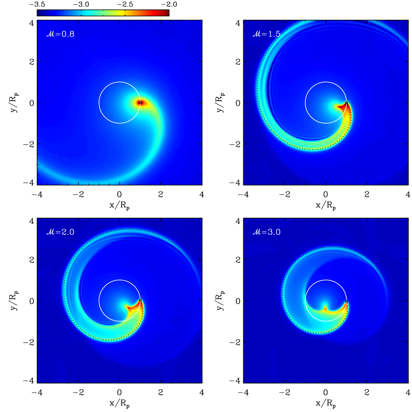
Figure 1.— Steady-state distributions of the perturbed density in logarithmic color scale on the $x$–$y$ plane at $t/t_{\rm orb}=1$ for low-mass perturbers with $\mathcal{R}=0.05$ and $\mathcal{B}=5\times 10^{-4}$ ($\mathcal{A}=0.01)$. Colorbar labels $\log(\rho/\rho_{0}-1)$. The white circle in each panel denotes the orbit, while the small black circle near $(x,y)=(R_{p},0)$ marks the softening radius of the perturber. The spiral dotted lines for the supersonic cases draw the outer edges of the tails from the linear theory, eq. (B2) of KK07, which are in good agreement with the numerical results.

2. Numerical Method

We consider a massive perturber moving on a circular orbit through a gaseous medium, and study the gravitational response of the gas to the perturber and the resulting drag force. Similar work for low-mass perturbers on circular orbits and massive perturbers on straight-line trajectories was presented in KK07 and KK09, respectively. Since the DF timescale is usually much longer than the orbital time, the idealized circular orbit is a reasonable approximation to real curvilinear orbits. We assume that the background medium is unmagnetized, non-self-gravitating, and initially static and homogeneous with density $\rho_{0}$ and adiabatic sound speed $a_{0}$. We adopt an adiabatic equation of state with index $\gamma=5/3$. The perturber with mass $M_{p}$ moves with a constant angular velocity $\Omega_{p}$ along a circle with radius $R_{p}$ on the $z=0$ plane; the corresponding linear velocity is $V_{p}=R_{p}\Omega_{p}$. We represent the perturber using a Plummer potential

$$\Phi_{\scriptscriptstyle P}(\mbox{\boldmath{$x$}},t)=-\frac{GM_{p}}{(|\mbox{\boldmath{$x$}}-\mbox{\boldmath{$x_{p}$}}(t)|^{2}+r_{s}^{2})^{1/2}},\;\;\;{\rm for}\;t\geq 0,$$ (4)

where $r_{s}$ is the softening radius and $\mbox{\boldmath{$x_{p}$}}(t)=R_{p}(\cos\Omega_{p}t,\sin\Omega_{p}t,0)$ is the perturber location at time $t$ in the Cartesian coordinates $(x,y,z)$.

We take $R_{p}$, $a_{0}$, and $t_{\rm cross}=R_{p}/a_{0}$ as the units of length, velocity, and time, respectively, in our simulations. Then, our models are completely characterized by three dimensionless parameters: $\mathcal{R}\equiv r_{s}/R_{p}$, $\mathcal{M}\equiv V_{p}/a_{0}$, and

$$\mathcal{B}\equiv\frac{GM_{p}}{a_{0}^{2}R_{p}}=\mathcal{R}\mathcal{A},$$ (5)

which is the ratio of the Bondi radius to the orbital radius. Note that $\mathcal{R}$ is a new parameter introduced by the circular orbit, which is absent for perturbers on straight-line trajectories. For future purposes, we define a dimensionless parameter

$$\eta_{\scriptscriptstyle\mathcal{B}}\equiv\frac{\mathcal{B}}{\mathcal{M}^{2}-1},$$ (6)

similarly to $\eta_{\scriptscriptstyle\mathcal{A}}$ in equation (2). To explore the parametric dependence of the drag force on $\mathcal{R}$, $\mathcal{M}$, and $\mathcal{B}$ (or equivalently $\mathcal{A}$), we run a total of 65 three-dimensional simulations with $\mathcal{R}$ varying in the range of $0.025$–$0.4$, $\mathcal{M}$ in $0.5$–4, and $B$ from $5\times 10^{-4}$ to $4$ ($\mathcal{A}$ from 0.01 to 80). Our fiducial model has $\mathcal{R}=0.05$, $\mathcal{M}=2$, and $\mathcal{B}=0.5$. We use the orbital time $t_{\rm orb}=2\pi R_{p}/V_{p}=2\pi t_{\rm cross}/\mathcal{M}$ as the time unit of our presentation.

Figure 2.— (a) Temporal evolution of the dimensionless DF force for $\mathcal{R}=0.02$, $\mathcal{B}=5\times 10^{-4}$ ($\mathcal{A}=0.01)$, and $\mathcal{M}=0.8$, 1.5, 2.0, and 3.0. The drag force reaches a steady-state value within $\sim 2t_{\rm cross}$. (b) The mean drag force (solid circles), averaged over $t/t_{\rm cross}=2$–5, against the Mach number. The standard deviation is smaller than the size of the circles. The solid line plots the linear force formula (eq. [1]) with $V_{p}t=2R_{p}$ and $r_{\rm min}/r_{s}=1.5+0.7(\mathcal{M}-1.8)^{2}$ in good agreement with the numerical results.

We integrate the basic equations of ideal hydrodynamics using a modified version of the ZEUS code (Stone & Norman, 1992), parallelized on a distributed-memory platform. Our simulations domain is a rectangular box which spans the region $-10R_{p}\leq x,y,z\leq 10R_{p}$. We construct a logarithmically spaced Cartesian grid with $512^{3}$ zones, with spacings of $0.0075R_{p}$, $0.018R_{p}$, and $0.11R_{p}$ at $|x|/R_{p}=0$, 1, and 10, respectively. For some selected parameters, we have also run low-resolution simulations with $256^{3}$ zones and checked that the resulting drag forces agree, within a few percents, with those from the high-resolution models. We adopt the outflow boundary conditions at all the boundaries and run the simulations typically up to $15t_{\rm cross}$. The simulation outcomes are insensitive to the box size and the boundary conditions we adopt since it takes about $\sim 20t_{\rm cross}$ for sound waves to travel across the simulation box, while the drag forces saturate typically within $\sim 0.5t_{\rm orb}\sim(2-3)t_{\rm cross}$.

3. Linear Cases

The time-dependent linear-perturbation analyses for the wakes of low-mass perturbers usually consider a point-mass object with vanishing $r_{s}$ in equation (4), which in turn requires to introduce the cut-off radius $r_{\rm min}$ in the linear DF force formula (e.g, Just & Kegel 1990; Ostriker 1999; KK07). On the other hand, one has to adopt a non-zero value for the softening radius in numerical simulations, making the DF force dependent on $r_{s}$ in the linear regime. To explore how the perturber mass affects the drag force in comparison with the linear theory, therefore, it is necessary to find a proper relationship between $r_{s}$ and $r_{\rm min}$ that makes the numerical results consistent with the analytic predictions when $\mathcal{B}\ll 1$. For this purpose, we present in this section the results of numerical simulations for low-mass perturbers with $\mathcal{B}=5\times 10^{-4}$ ($\mathcal{A}=0.01$) and $\mathcal{R}=0.05$ as functions of $\mathcal{M}$.

Figure 1 shows the snapshots of density wakes on the $x$–$y$ plane at $t/t_{\rm orb}=1$ for $\mathcal{M}=0.8$, 1.5, 2, and 3 cases. The perturber in each frame is moving along the white circle in the counterclockwise direction. For subsonic perturbers, the circular orbit makes the density wakes curved along their orbits that would otherwise remain symmetric with respect to the line of motion. For supersonic models, the perturber is able to overtake its own wake, creating a strong trailing tail bounded by Mach waves (KK07). As the Mach number increases from unity, the opening angle of the head of the curved Mach cone deceases, while the tail thickens. The dotted lines for the supersonic models plot equation (B2) of KK07 for the shape of the tail, which are in excellent agreement with the outer boundaries of the tails produced in the simulations. Nevertheless, the finite perturber size in the latter makes the tail boundaries broader compared to the point-mass counterparts with $r_{s}=0$.

For a given density wake $\rho(\mbox{\boldmath{$x$}},t)$, it is straightforward to calculate the gravitational drag force on the perturber by evaluating the integral

$$F(t)=\int\frac{GM_{\scriptscriptstyle P}(|\mbox{\boldmath{$x$}}-\mbox{\boldmath{$x$}}_{p}|)\rho(\mbox{\boldmath{$x$}},t)(\mbox{\boldmath{$x$}}-\mbox{\boldmath{$x$}}_{p})\cdot\hat{\varphi}}{|\mbox{\boldmath{$x$}}-\mbox{\boldmath{$x$}}_{p}|^{3}}\ d^{3}\mbox{\boldmath{$x$}},$$ (7)

where $M_{\scriptscriptstyle P}(r)=M_{p}r^{3}/(r^{2}+r_{s}^{2})^{3/2}$ is the mass distribution of the Plummer sphere and $\hat{\varphi}={\mbox{\boldmath{$\hat{z}$}}}\times{\mbox{\boldmath{$\hat{x}_{p}$}}}$ is the unit vector in the azimuthal direction. Figure 2a shows the temporal evolution of $F(t)$ for the cases shown in Figure 1. The friction force saturates to a constant value in less than $\sim 2t_{\rm cross}$; the amplitudes of fluctuations in $F$ are less than $1\%$ of the mean values. This is unlike in the linear-trajectory models where the DF force on a supersonic perturber increases logarithmically with time, since the whole density wake growing in size with time is located behind the perturber. The region of influence in the circular-orbit models expands at a sonic speed from the orbit center. Consequently, the far-field wake in these models is more or less spherically symmetric and thus does not contribute to the DF force much. Figure 2b plots as solid circles the steady-state drag forces against $\mathcal{M}$ for low-mass perturbers with $\mathcal{B}=5\times 10^{-4}$ ($\mathcal{A}=0.01$) and $\mathcal{R}=0.05$. The solid line represents the fit using equation (1) with

$$r_{\rm min}/r_{s}=1.5+0.7(\mathcal{M}-1.8)^{2},$$ (8)

which is in good agreement with the numerical results. In what follows, we will use equation (8) as the cut-off radius when we compare the numerical DF forces with the analytic estimates.

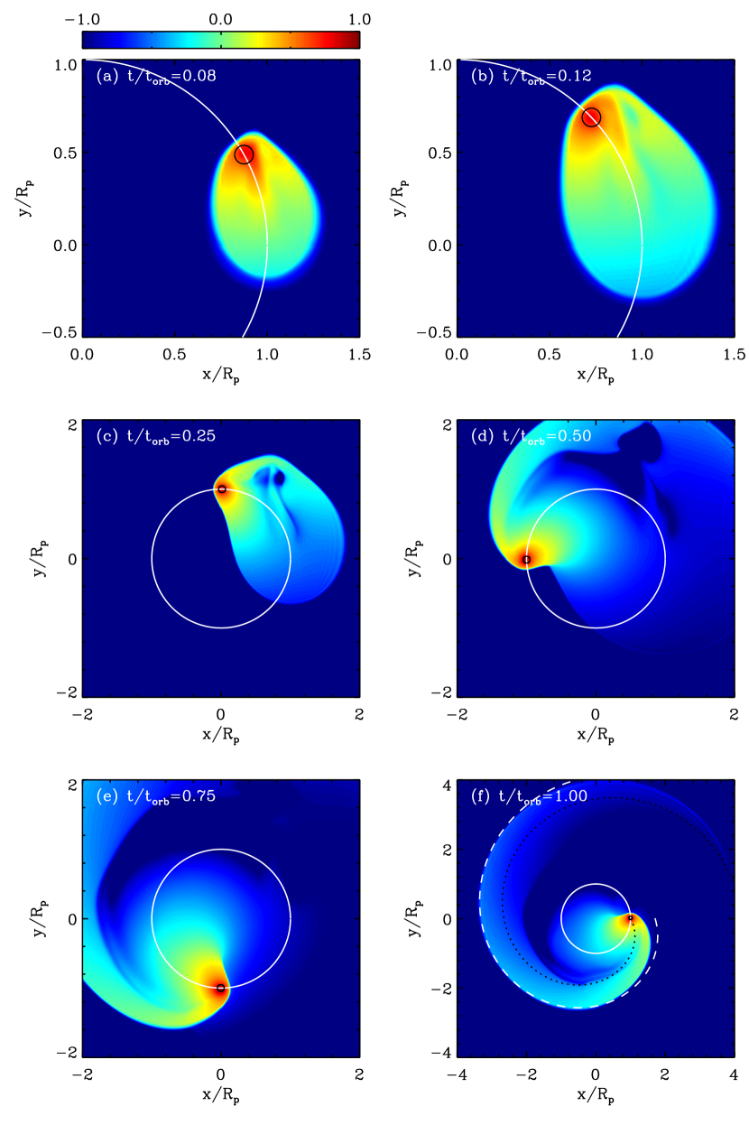
Figure 3.— Density shapshots on the $x$–$y$ plane for a supersonic model with $\mathcal{M}=2$, $\mathcal{R}=0.05$, and $\mathcal{B}=0.5$ ($\mathcal{A}=10$). The size of the region displayed differs from panel to panel for clarity. The white circle or part of it in each panel denotes the orbit, while the small black circle marks the softening radius of the perturber. In (f), the black dotted line plots equation (B2) of KK07 for the linear tail, while the white dashed line that matches the outer edge of the nonlinear tail is drawn by rotating the former by $75^{\circ}$ in the counterclockwise direction. Colorbar labels $\log(\rho/\rho_{0}-1)$. See text for detail.

4. Nonlinear Cases

4.1. Wake Evolution

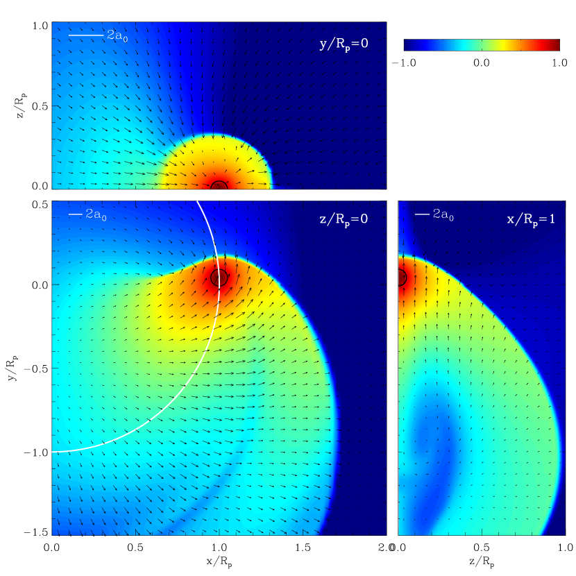
Figure 4.— Quasi-steady distributions of the density wake and velocity field, seen in the inertial frame, on the $x/R_{p}=1$ (bottom right), $y=0$ (top left), and $z=0$ (bottom left) planes for a supersonic model with $\mathcal{M}=2$, $\mathcal{R}=0.05$, and $\mathcal{B}=0.5$ ($\mathcal{A}=10$) at $t/t_{\rm orb}=2$. The small black circle marks the softening radius of the perturber, while the white curve in the bottom left panel draws the perturber orbit. The length of the line segment shown in the upper left corner of each panel, corresponding to twice the sound speed, measures the size of the velocity vectors. Colorbar labels $\log(\rho/\rho_{0}-1)$.

We now focus on the cases with very massive perturbers. Figure 3 plots the snapshots of logarithmic density on the $x$–$y$ plane for our standard model with $\mathcal{R}=0.05$, $\mathcal{M}=2$, and $\mathcal{B}=0.5$ ($\mathcal{A}=10$). In each panel, the white line draws the perturber orbit, while the small circle in black marks the perturber location with its size corresponding to the softening radius $r_{s}$. The perturber is initially located at $(x,y)=(R_{p},0)$ and orbits in the counterclockwise direction. Note that the size of the region displayed in Figure 3 differs from panel to panel for clear presentation. The evolution of the density wake at early phase is qualitatively similar to the linear-trajectory cases described in KK09. An introduction of the perturber at $t=0$ provides the background gas with strong perturbations that readily develop into a bow shock. The incident gas along the line of motion is shocked and gathered near the perturber. This sets up a strong pressure gradient in the region between the shock and the perturber, which in turn causes the shock to slowly move away from the perturber in the upstream direction until it reaches an equilibrium position. Some gas flowing with a non-zero impact parameter is gradually pulled by the perturber, adding to the density at the rear side (Fig. 3$a$). Due to the strong gravity, the material piled up at the backside is pulled back toward the perturber, creating a strong counterstream along the line of motion as well as a surrounding vortex ring (see KK09).

For the linear-trajectory cases, KK09 has shown that the counterstream slows down due in part to the strong pressure gradient established near the perturber and in part to a buoyant expansion of the vortex ring in the lateral direction. The interaction of the counterstream with the shocked gas causes the bow shock to move back and forth around an equilibrium position. During this time, the vortex ring also undergoes an overstable oscillation whose amplitude grows secularly with time. When the vortex ring moves out beyond a half of the Hoyle-Lyttleton radius $r_{\rm HL}=2GM_{p}/V_{p}^{2}$, it becomes less gravitationally bound and soon swept downstream by the ram pressure of the incident gas, leaving a near-hydrostatic envelope surrounding the perturber. This is how a density wake enters into a quasi-steady state in the linear-trajectory cases. For the circular-orbit cases, however, the line of perturber motion keeps changing with time. With the perturber displaced from the direction of the counterstream, the counterstream is virtually unhindered and travels almost straight in the direction tangent to the orbit, producing the protruding region in the wake at $x\approx y\approx 0.85R_{p}$ shown in Figure 3$b$ . Consequently, the vortex ring manifesting its presence by low density at $x/R_{p}=0.6$–$0.9$ and $y/R_{p}=1.1$–$1.2$ in Figure 3$c$ that was carried by the counterstream decouples from the perturber, promptly leaving a quasi-static density distribution around the perturber. Note that the time to form a near-hydrostatic envelope is about $\sim 0.5t_{\rm orb}\approx 30r_{s}/a_{0}$, which is shorter than in the linear-trajectory cases by about an order of magnitude.

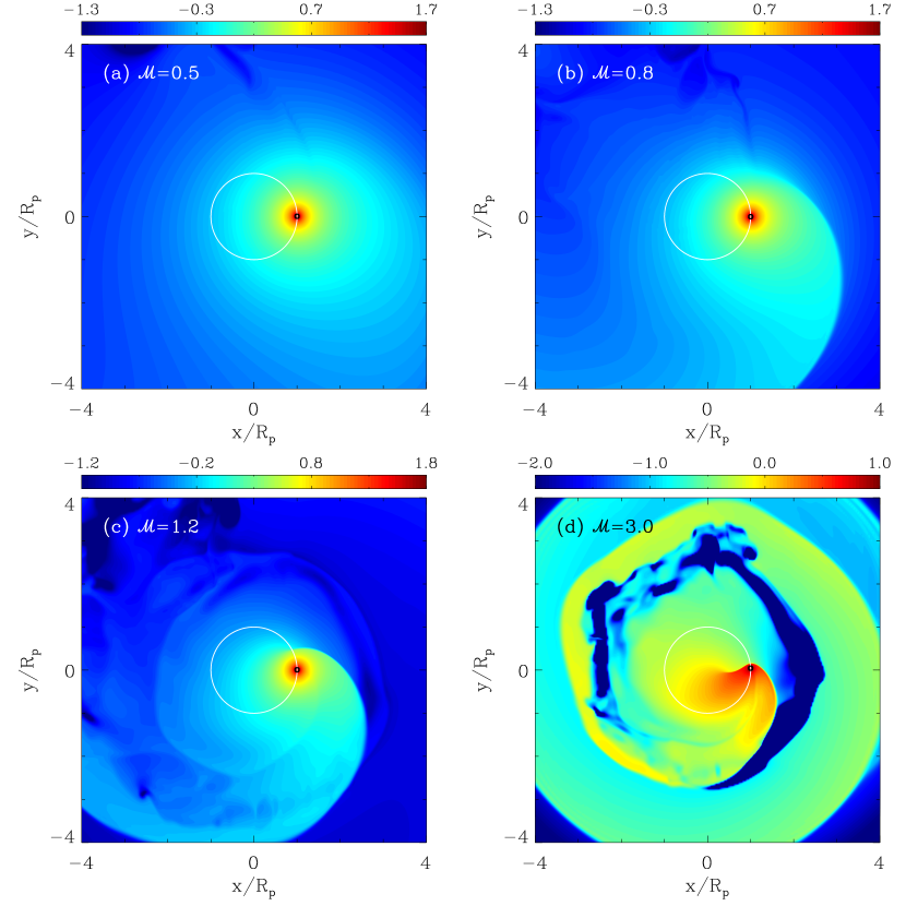
Figure 5.— Distributions of quasi-steady density wakes with differing $\mathcal{M}$ on the $x$–$y$ plane, with the perturber located at $(x,y,z)=(R_{p},0,0)$. All the models have $\mathcal{R}=0.05$ and $\mathcal{B}=1$. The white circle in each panel shows the orbit. Colorbar labels $\log(\rho/\rho_{0}-1)$.

While the density distribution near the perturber is nearly spherical, a part of the wake outside the orbit is pushed radially outward by the counterstream, developing a trailing tail on the $x$–$y$ plane. As the counterstream weakens, the low-density regions associated with the vortex ring first merge together and are then stretched along the orbit as the perturber continues the orbital motion (Fig. 3$d,e$). In the low-mass perturber cases with $\mathcal{A}\ll 1$, the wake tail is created by the overlapping of the Mach cone and the sonic sphere (KK07). In the nonlinear cases, however, it is the low-density regions produced by the counterstream that separate the tail from the rest of the wake. The black dotted curve in Figure 3f plots the shape of the linear tail, as in Figure 1, which does not match the outer edge of the nonlinear tail in our fiducial model. Instead, the latter is well matched by rotating the former by $75^{\circ}$ in the counterclockwise direction, shown as the dashed curve.

4.2. Quasi-steady Density Wakes

Figure 6.— Density profiles of steady-state wakes as functions of the distance $l$ from the perturber center along the azimuthal direction for (a) models with fixed $\mathcal{R}=0.05$ and varying $\mathcal{B}$ and (b) models with fixed $\mathcal{B}=1$ and varying $\mathcal{R}$. All the models have $\mathcal{M}=2$. In (a), the dotted lines give the respective density distributions under the assumption of hydrostatic equilibrium, while the numerical results are drawn as the solid lines. Note that varying $\mathcal{R}\lower 2.0pt\hbox{$\;\buildrel\scriptstyle<\over{\scriptstyle\sim}\;$}0.1$ changes the density only in the very central parts of the hydrostatic envelopes.

Figure 4 shows the quasi-steady distributions of the density as well as the velocity field, seen in the inertial frame, on the $x/R_{p}=1$, $y=0$, and $z=0$ planes for our fiducial model at $t/t_{\rm orb}=2$. The colorbar labels the perturbed density in logarithmic scale. The size of the short line segment shown in the upper left corner of each panel, corresponding to twice the sound speed, measures the amplitudes of the velocity vectors. The density wake consists of a spherical envelope surrounding the perturber, a detached bow shock, and an extended low-density region at the rear side. The envelope is almost hydrostatic, as evidenced by low-amplitude velocity vectors in the $y=0$ plane to which the perturber motion is perpendicular instantaneously. The bow shock standing outside the orbit, in the $z=0$ plane, is just a curved version of that in the linear trajectory counterpart and extends to large radii $R=(x^{2}+y^{2})^{1/2}$ in the orbital plane. On the other hand, the (almost planner) shock located inside the orbit gradually weakens at small $R$ and terminates at $R/R_{p}\sim 0.5$–$0.6$ since the speed of the density wake corotating with the perturber becomes subsonic there. The low-density regions delineating the tail seen at $t/t_{\rm orb}=1$ (Fig. 3f) are less apparent in Figure 4 as they diffuse out over time by pressure gradients. While the velocity just ahead of the perturber is parallel to the direction of the instantaneous perturber motion, the direction of gas motions at the perturber location and the immediate behind it are inclined about $30^{\circ}$–$50^{\circ}$ from the tangential direction. This implies that the gas in the downstream side retains the information on the direction of perturber motion in the past.

Figure 5 displays changes in the quasi-steady density wakes with varying $\mathcal{M}$ on the orbital plane for models with $\mathcal{R}=0.02$ and $\mathcal{B}=1$ ($\mathcal{A}=20$). In each panel, the perturber located at $x/R_{p}=1$ and $y=0$ is moving along the white circle in the counterclockwise direction. When $\mathcal{M}=0.5$, the density distribution is circular near the perturber and becomes eccentric away from it, with the minor axis parallel to the line of motion. Still, there exists a slight excess of the perturbed density in the rear side, giving rise to a non-vanishing (but small) DF force. Compared to the $\mathcal{M}=0.5$ model, the model with $\mathcal{M}=0.8$ has a larger density excess at the backside. While the perturber is subsonic in this model, a strong gravitational pull is able to accelerate the background gas to a near-transonic speed, creating a weak shock outside the orbit. The shape of the density wake in the $\mathcal{M}=1.2$ model is similar to that for the $\mathcal{M}=2.0$ model, although the former has a larger peak density and a larger distance of the detached bow shock. As $\mathcal{M}$ increases further, both the detached shock distance and the size of the hydrostatic envelope decrease. The ring-like low-density gap at $R/R_{p}\sim 2$ in Figure 5d is a remnant of the counterstream that was stretched along the orbit. With large values of $\mathcal{M}$ and $\mathcal{B}$, the counterstream in this model was so strong that the deep gap has not been filled in yet.

In order to check whether the density wake near the perturber is in hydrostatic equilibrium, we plot in Figure 6 the density profiles of steady-state wakes as functions of distance $l$ measured from the perturber location along the azimuthal direction in models with $\mathcal{M}=2$. The solid lines in Figure 6a give the simulation results for perturbers with fixed $\mathcal{R}=0.05$ and differing $\mathcal{B}$. The sharp discontinuity in each curve is due to the presence of the bow shock. The dotted lines draw the density distributions of the hydrostatic spheres

$$\rho(l)=\rho_{c}\left\{1+\frac{(\gamma-1)a_{0}^{2}\mathcal{B}}{a_{c}^{2}\mathcal{R}}\left[\frac{r_{s}}{(l^{2}+r_{s}^{2})^{1/2}}-1\right]\right\}^{1/(\gamma-1)},$$ (9)

where $\rho_{c}$ and $a_{c}$ denote the density and adiabatic sound speed at $l=0$ (i.e., the perturber center), respectively (KK09). These are in good agreement with the density profiles of the steady-state wakes in our simulations, suggesting that the envelopes are indeed almost hydrostatic. Figure 6b shows how the density profile varies with $\mathcal{R}$. When $\mathcal{B}=1$, the nonlinear effect is not significant in models with $\mathcal{R}>0.33$ since they have $\eta_{\scriptscriptstyle\mathcal{A}}<1$; the density jump occurring at $l\sim 0$ in the $\mathcal{R}=0.4$ model is more like a Mach wave rather than a shock. As $\mathcal{R}$ decreases (or $\eta_{\scriptscriptstyle\mathcal{A}}$ increases), the density wake becomes increasingly nonlinear, producing a hydrostatic envelope and a detached bow shock. Note that the shock location is unchanged as long as $\mathcal{R}\lower 2.0pt\hbox{$\;\buildrel\scriptstyle<\over{\scriptstyle\sim}\;$}0.2$ (or $\eta_{\scriptscriptstyle\mathcal{A}}\lower 2.0pt\hbox{$\;\buildrel\scriptstyle>\over{\scriptstyle\sim}\;$}2$). When the density is highly nonlinear, the strong gravity associated with small $r_{s}$ increases the density only in the small regions within $\lower 2.0pt\hbox{$\;\buildrel\scriptstyle<\over{\scriptstyle\sim}\;$}(1-2)r_{s}$. Since this core region is spherically symmetric, the resultant DF force becomes independent of $\mathcal{R}$ provided $\eta_{\scriptscriptstyle\mathcal{A}}\lower 2.0pt\hbox{$\;\buildrel\scriptstyle>\over{\scriptstyle\sim}\;$}2$. We will show this directly in §4.4 below.

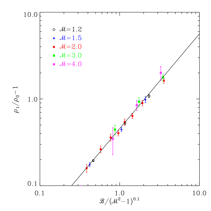
Figure 7.— Modified background density $\rho_{1}$ ahead of the bow shock in models with $\mathcal{R}=0.05$. Various symbols and errorbars give the means and standard deviations of the preshock density in the regions with $\Delta l/R_{p}=0.5$–$1.5$ from the detached shock. The solid line plots the best fit given by equation (10).

Unlike in the linear-trajectory cases where a perturber travels through an undisturbed medium, it is inevitable that a circular-orbit perturber enters the backside of its own wake before completing one orbit. In the circular-orbit cases, therefore, the density ahead of the bow shock differs from the undisturbed density $\rho_{0}$ and depends considerably on $\mathcal{B}$, as Figure 6a illustrates. The enhanced preshock density can alternatively be interpreted as arising from the response of the background gas to the orbit-averaged gravitational potential of the perturber $\langle\Phi_{\scriptscriptstyle P}\rangle\equiv\int_{0}^{t_{\rm orb}}\Phi_{\scriptscriptstyle P}(t)dt/t_{\rm orb}$, which is centered at the orbit center. In this sense, the enhanced preshock density $\rho_{1}$ acts as a modified background density to a circular-orbit perturber with the gravitational potential $\Phi_{\scriptscriptstyle P}-\langle\Phi_{\scriptscriptstyle P}\rangle$. To quantify $\rho_{1}$, we take a spatial average of the preshock density in quasi-steady state over the region with $(l-\delta)/R_{p}=0.5$–$1.5$ along the orbit, where $\delta$ denotes the location of the detached shock. Figure 7 plots the resulting $\rho_{1}$ for models with $\mathcal{R}=0.05$, with errorbars representing the standard deviations. The solid line is the best fit

$$\frac{\rho_{1}}{\rho_{0}}=1+\frac{0.46\mathcal{B}^{1.1}}{(\mathcal{M}^{2}-1)^{0.11}},$$ (10)

showing that the change in the background density to circular-orbit perturbers is almost linearly proportional to $\mathcal{B}$. Since $\rho_{1}$ is quite insensitive to $\mathcal{M}$, the $\mathcal{M}$-dependence of $\rho_{1}$ in equation (10) can be ignored.

4.3. Detached Shock Distance

Figure 8.— Temporal evolution of (a) the detached shock distances $\delta$ and (b) the DF forces $F$ for models $\mathcal{R}=0.05$ and $\mathcal{M}=2$. Both $\delta$ and $F$ increase rapidly with time initially and then saturate at $t/t_{\rm orb}\sim 0.5$ to equilibrium values with some fluctuations. The dimensionless drag force decreases with $\mathcal{B}$ for $0.05<\mathcal{B}<2$ due to the nonlinear effect.

In laboratory experiments and hydrodynamic theories, supersonic flows over a blunt-body generate a detached bow shock when the maximum angle allowed in the postshock flows is smaller than the nose angle (e.g., Liepmann & Roshko 1957; Shu 1992). Although a perturber in our models does not hold any defined surface and merely provides gravitational perturbations to the background gas, a spherical envelope formed around it nevertheless sends off pressure waves into the upstream direction, acting as an obstacle to the incoming gas. Since the nose-angle of a spherical body is $90^{\circ}$, the shock should be detached in our nonlinear supersonic models. Figure 8a plots the time evolution of the detached shock distance $\delta$ for some selected models with $\mathcal{R}=0.02$ and $\mathcal{M}=2$. Note that $\delta$ initially increases rapidly and then saturates at $t/t_{\rm orb}\sim 0.5$ to an equilibrium value with some fluctuations. The quasi-steady value of $\delta$ becomes larger as the perturber mass increases.

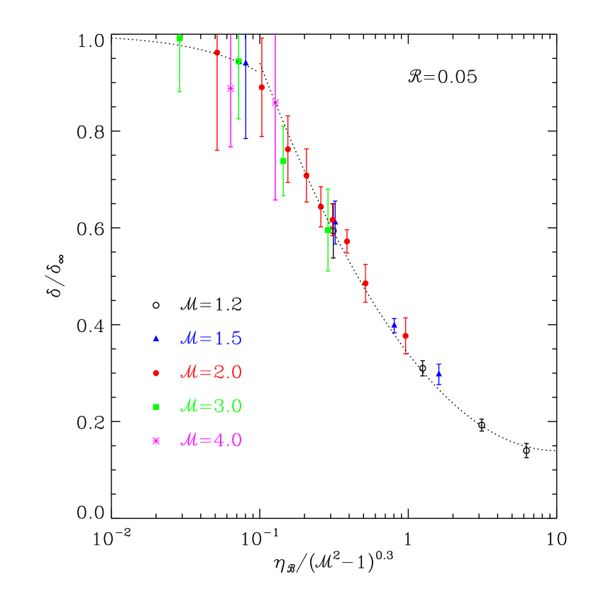
Figure 9.— Quasi-steady values of the detached shock distances $\delta$ of circular-orbit perturbers relative to those, $\delta_{\infty}$, of linear-trajectory perturbers. Various symbols and errorbars give the means and standard deviations of $\delta/\delta_{\infty}$ over $t/t_{\rm orb}=1$–$3$. The dotted curves, expressed as equation (12), are the best fits to the numerical results.

For massive perturbers moving on a straight-line trajectory, KK09 found that the detached shock distance is given empirically by

$$\delta_{\infty}=r_{s}\eta_{\scriptscriptstyle\mathcal{A}}=\frac{GM_{p}}{a_{0}^{2}(\mathcal{M}^{2}-1)}.$$ (11)

This can be interpreted by the balance between the postshock thermal energy ($\propto a_{0}^{2}\mathcal{M}^{2}$) and the gravitational potential energy ($\propto-GM_{p}/\delta$) at the shock location for strong shocks ($\mathcal{M}\gg 1$). To study how the circular obit affects the standoff distance of the shock, we take a time average of $\delta(t)$ over $t/t_{\rm orb}\sim 1$–$3$ and plot $\delta/\delta_{\infty}$ in Figure 9 as various symbols. Again, errorbars indicate the standard deviations of $\delta(t)$ during this time interval. The numerical results show that the detached shock distances in the circular orbits are in general smaller than those in the linear-trajectory cases. This is likely because the continuous change in the direction of perturber motion effectively reduces the forward momentum of the incident gas near the perturber, as illustrated by the spatially-varying velocity field in the wake shown in Figure 4. In this case, the ram pressure of the incoming flow is able to push the shock front toward the perturber, making $\delta$ smaller. The modified background density and sound speed discussed in §4.2 might affect $\delta$ as well. We fit our results using

$$\frac{\delta}{\delta_{\infty}}=\left\{\begin{array}[]{ll}1-0.8\Lambda,&\;\;\;\;\;\;\;\;\;\,\Lambda<0.1,\\ 0.14+0.2(1-\log\Lambda)^{2},&0.1<\Lambda<10,\end{array}\right.$$ (12)

with $\Lambda\equiv\eta_{\scriptscriptstyle\mathcal{B}}/(\mathcal{M}^{2}-1)^{0.3}$, which is plotted as dotted lines. As expected, $\delta/\delta_{\infty}\rightarrow 1$ as $\Lambda\rightarrow 0$ corresponding to $R_{p}\rightarrow\infty$, although models with $\Lambda\lower 2.0pt\hbox{$\;\buildrel\scriptstyle<\over{\scriptstyle\sim}\;$}0.1$ are weakly nonlinear and have $\delta$ comparable to or less than $r_{s}$. Since $\delta_{\infty}/R_{p}=\eta_{\scriptscriptstyle\mathcal{B}}$, equation (12) indicates that $\delta$ increases with $\Lambda$, although its increasing rate slows down as $\Lambda\rightarrow 10$ where $\delta$ becomes comparable to $R_{p}$.

4.4. Drag Force

For our nonlinear models, we calculate the DF force on a perturber due to its own induced wake. Figure 8b illustrates the temporal changes of the dimensionless drag force $\mathcal{I}\equiv F/[4\pi\rho_{0}(GM_{p}/a_{0})^{2}]$ in models with $\mathcal{M}=2$ and $\mathcal{R}=0.02$ and varying $\mathcal{B}$. The drag force reaches a quasi-steady value in less than one orbit, although it exhibits some fluctuations for large $\mathcal{B}$. This is markedly different from the cases of straight-line trajectories where the drag force increases logarithmically with time. The quasi-steady value of $\mathcal{I}$ is almost independent of $\mathcal{B}$ when $\mathcal{B}\lower 2.0pt\hbox{$\;\buildrel\scriptstyle<\over{\scriptstyle\sim}\;$}0.05$, decreases with $\mathcal{B}$ for $0.05\lower 2.0pt\hbox{$\;\buildrel\scriptstyle<\over{\scriptstyle\sim}\;$}\mathcal{B}\lower 2.0pt\hbox{$\;\buildrel\scriptstyle<\over{\scriptstyle\sim}\;$}2$, and becomes again insensitive to $\mathcal{B}$ when $\mathcal{B}\lower 2.0pt\hbox{$\;\buildrel\scriptstyle>\over{\scriptstyle\sim}\;$}2$. The behavior of $\mathcal{I}$ with $\mathcal{B}$ is a consequence of the circular orbit combined with the nonlinear effect. The size of a hydrostatic envelope in a nonlinear density wake, as measured by the detached shock distance, becomes larger with increasing $\mathcal{B}$, which makes the drag force smaller owing to the front-back symmetry in the wake. At the same time, the circular orbit draws the background material toward the orbit center and increases the density in the preshock region, which in turn tends to increase the drag force. For models with $\mathcal{B}\lower 2.0pt\hbox{$\;\buildrel\scriptstyle<\over{\scriptstyle\sim}\;$}2$ (so that $\rho_{1}/\rho_{0}\lower 2.0pt\hbox{$\;\buildrel\scriptstyle<\over{\scriptstyle\sim}\;$}2$), the nonlinear effect dominates and $\mathcal{I}$ decreases with $\mathcal{B}$. When $\mathcal{B}\lower 2.0pt\hbox{$\;\buildrel\scriptstyle>\over{\scriptstyle\sim}\;$}2$, on the other hand, the enhancement of the background density becomes significant enough to compensate for the nonlinear effect, making $\mathcal{I}$ unchanged with $\mathcal{B}$. As we will show below, the DF force scales well with $\mathcal{B}$ when $\rho_{1}/\rho_{0}$ is taken into account.

Compared to the linear-trajectory cases, the circular orbit introduces an additional length scale, $R_{p}$, so that it is interesting to explore the dependence of the drag force upon $\mathcal{R}$. Figure 10a plots as various symbols and errorbars the mean values and standard deviations of the drag forces averaged over $t/t_{\rm orb}=2$–4 for models with $\mathcal{M}=2$. Note that the drag force is normalized by $\rho_{1}$ instead of $\rho_{0}$. The dotted line marked with $\eta_{\scriptscriptstyle\mathcal{A}}=2$ demarcates the parameter space into two parts such that the models shown in the lower-left region are fully nonlinear with $\eta_{\scriptscriptstyle\mathcal{A}}>2$, while those in the upper-right region are in the linear or weakly nonlinear regime. The normalized drag force on weakly-nonlinear perturbers with $0.7<\eta_{\scriptscriptstyle\mathcal{A}}<2$ is usually larger than that on low-mass perturbers with $\eta_{\scriptscriptstyle\mathcal{A}}<0.7$ because the density wakes in the former are distributed closer to the perturber (KK09). In highly-nonlinear models with $\eta_{\scriptscriptstyle\mathcal{A}}>2$ (or $\eta_{\scriptscriptstyle\mathcal{B}}>2\mathcal{R}$), on the other hand, the DF force becomes essentially independent of $\mathcal{R}$. This is of course because the change in $r_{s}$ affects the wake only within a small region close to the perturber where the density is spherically symmetric, making a negligible contribution to the drag force (see §4.2).

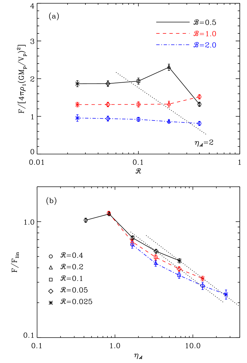
Figure 10.— Normalized DF forces averaged over $t/t_{\rm orb}=2$–$4$ for models with $\mathcal{M}=2$ and various $\mathcal{B}$ and $\mathcal{R}$ as functions of (a) $\mathcal{R}$ and (b) $\eta_{\scriptscriptstyle\mathcal{A}}$. The dotted line corresponding to $\eta_{\scriptscriptstyle\mathcal{A}}=2$ in (a) separates the domain into two parts such that the models at the lower-left part are fully nonlinear. Dotted lines in (b) have a slope of $-0.5$ and connect the numerical results for $\mathcal{R}=0.05$ and 0.025 models quite well.

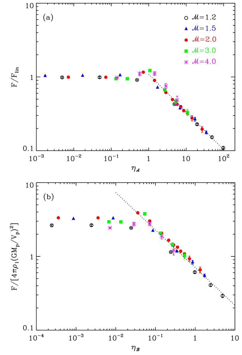
Figure 11.— (a) DF forces on supersonic perturbers with $\mathcal{R}=0.05$ normalized by the linear drag force as a function of $\eta_{\scriptscriptstyle\mathcal{A}}$. Various symbols and their errorbars give the means and standard deviations of $F/F_{\rm lin}$ for $t/t_{\rm orb}=2$–$4$. The dotted line indicates a slope of $-0.5$. (b) The same data as in (a) but with different normalization and as a function of $\eta_{\scriptscriptstyle\mathcal{B}}$. The dotted line shows the best fit to the numerical results for $\eta_{\scriptscriptstyle\mathcal{B}}>0.1$ and is given by equation (14).

Figure 10b plots $F/F_{\rm lin}$ versus $\eta_{\scriptscriptstyle\mathcal{A}}$ for the same models shown in Figure 10a. Note again that $\rho_{0}$ in equation (1) for $F_{\rm lin}$ is replaced by $\rho_{1}$. For given $\mathcal{B}$ (so that increasing $\eta_{\scriptscriptstyle\mathcal{A}}$ corresponds to decreasing $\mathcal{R}$), $F/F_{\rm lin}$ decreases logarithmically with increasing $\eta_{\scriptscriptstyle\mathcal{A}}>2$. This is because $\eta_{\scriptscriptstyle\mathcal{A}}\propto\mathcal{R}^{-1}$ for fixed $\mathcal{B}$ and $\mathcal{M}$, leading to $F_{\rm lin}\propto\ln\eta_{\scriptscriptstyle\mathcal{A}}$, while $F$ is constant for $\eta_{\scriptscriptstyle\mathcal{A}}>2$. For fixed $\mathcal{R}$ (so that increasing $\eta_{\scriptscriptstyle\mathcal{A}}$ corresponds to increasing $\mathcal{B}$), $F/F_{\rm lin}\propto\eta_{\scriptscriptstyle\mathcal{A}}^{-0.5}$, as illustrated by two dotted lines connecting the numerical results for $\mathcal{R}=0.05$ and 0.025, respectively. Figure 11a plots $F/F_{\rm lin}$ for all of our supersonic models with $\mathcal{R}=0.05$. Obviously, $F/F_{\rm lin}\approx 1$ for low-mass perturbers with $\eta_{\scriptscriptstyle\mathcal{A}}<0.7$. The dotted line is the best fit

$$\frac{F}{F_{\rm lin}}=1.1\eta_{\scriptscriptstyle\mathcal{A}}^{-0.5},{\rm\;\;for\;}\eta_{\scriptscriptstyle\mathcal{A}}>2,$$ (13)

to the numerical results for nonlinear, circular-orbit perturbers, which is very similar to equation (3) for massive, linear-trajectory perturbers.

In order to apply equation (13) to estimate the decay timescale, one needs to specify the softening radius which is not directly observable in most astronomical systems. In addition, equation (13) is applicable only when $\mathcal{R}=0.05$ since $F$ on highly massive perturbers is independent of $r_{s}$, while $F_{\rm lin}$ diverges as $r_{s}\rightarrow 0$. For practical use in various situations, therefore, it is desirable to have an expression of $F$ that does not rely on $r_{s}$. For this purpose, we plot in Figure 11b the dimensionless DF forces as a function of $\eta_{\scriptscriptstyle\mathcal{B}}$ for all supersonic models with $\mathcal{R}=0.05$. The dotted line is our fit to the nonlinear part using

$$F=\frac{4\pi\rho_{1}(GM_{p})^{2}}{V_{p}^{2}}\left(\frac{0.7}{\eta_{\scriptscriptstyle\mathcal{B}}^{0.5}}\right),{\rm\;\;for\;}\eta_{\scriptscriptstyle\mathcal{B}}>0.1,$$ (14)

with $\rho_{1}$ given by equation (10). For the models with $\eta_{\scriptscriptstyle\mathcal{B}}<0.1$, equations (1) and (8) with $V_{p}t=2R_{p}$ provide a good estimate of $F$ that depends on $r_{s}$.

5. Summary and Discussion

DF due a gaseous medium may play a central role in removing angular momentum from astronomical objects in orbital motions, causing them to spiral in toward the orbit center. In this paper, we use three-dimensional hydrodynamic simulations to explore the gravitational wake and the associated drag force on a very massive perturber with mass $M_{p}$ moving at speed $V_{p}$ on a circular orbit with radius $R_{p}$. This work extends our previous studies that considered low-mass, circular-orbit perturbers (KK07) and high-mass, linear-trajectory perturbers (KK09). The background medium is assumed to be uniform with density $\rho_{0}$ and the sound speed $a_{0}$, adiabatic with index $\gamma=5/3$, non-self-gravitating, non-rotating, and unmagnetized. The perturber is represented by a Plummer sphere with softening radius $r_{s}$. Our models are characterized completely by three dimensionless parameters: $\mathcal{R}=r_{s}/R_{p}$, $\mathcal{M}=V_{p}/a_{0}$, and $\mathcal{B}=GM_{p}/(a_{0}^{2}R_{p})$. We run a total of 65 models that differ in $\mathcal{R}$, $\mathcal{M}$, and $\mathcal{B}$, and obtain the dependence of the drag force on these parameters.

For our supersonic models, the density wake of a massive perturber reaches a quasi-steady state typically in $\sim 0.5t_{\rm orb}$, about 10 times faster than the linear-trajectory cases. A quasi-steady density wake consists of a spherical envelope surrounding the perturber, a detached bow shock in the upstream direction, and an extended low-density region in the rear side. The envelope is almost hydrostatic, providing a negligible contribution to the DF force. Compared to the linear-trajectory cases, an orbit-averaged gravitational potential of a circular-orbit perturber is able to gather the background gas toward the orbit center, effectively increasing the background density ahead of the bow shock. Equation (10) describes the modified preshock density $\rho_{1}$, showing that density enhancement in the preshock region is almost linearly proportional to $\mathcal{B}$ and depends weakly on $\mathcal{M}$.

Strong perturbations sent off from a massive perturber develop into a bow shock through which the upstream supersonic flow becomes subsonic. Since the density wake in a quasi-steady state forms a pattern that is corotating with the perturber at a constant angular speed, the incident flow outside the orbit is supersonic to a perturber with $\mathcal{M}>1$. This naturally produces a bow shock outside the orbit that is simply a curved version of that in the linear-trajectory counterpart. Formation of a weak bow shock outside the orbit is possible even for a subsonic perturber with $\mathcal{M}\lower 2.0pt\hbox{$\;\buildrel\scriptstyle>\over{\scriptstyle\sim}\;$}0.8$ for which the incident flow is accelerated to near-transonic speeds. On the other hand, the motion of the steady-state wake is subsonic to the gas near the orbit center, even when $\mathcal{M}>1$. This makes the bow shock gradually weaken at small radii, eventually terminating somewhere inside the orbit. The detached shock distance measured along the tangential direction is generally smaller than in the liner-trajectory counterpart since the continuous change in the direction of the perturber motion effectively reduces the forward momentum of the wake; equation (12) gives the algebraic fits to the numerical results for the detached shock distance.

Unlike in the linear-trajectory cases where the drag force increases logarithmically with time, the DF force in the circular orbits approaches a quasi-steady value in less than one orbit. The quasi-steady drag force is essentially independent of $\mathcal{R}$ as long as $\eta_{\scriptscriptstyle\mathcal{A}}>2$ (or $\eta_{\scriptscriptstyle\mathcal{B}}>2\mathcal{R}$) since the change in $r_{s}$ modifies the density wake only within $\sim(1-2)r_{s}$ from the perturber center, where the wake is almost spherically symmetric and thus has a negligible contribution to the drag force. For sufficiently massive perturbers, the presence of a near-hydrostatic envelope in the density wake also makes the nonlinear drag force smaller than the linear estimate. Since the choice of $r_{s}$ is uncertain in many practical applications, we fit the nonlinear drag force on a circular-orbit perturber using equation (14) that does not involve $r_{s}$.

That the nonlinear drag force in circular orbits is insensitive to the softening radius seems inconsistent with the results of KK09 for linear-trajectory perturbers. But, it does not. For the latter case, $r_{s}$ is in fact a lone length scale relative to which other length scales such as the Bondi radius and the distance traveled by the perturber are measured. It is then difficult to separate the effect of $r_{s}$ on the drag force from that of $M_{p}$ because the models depend on them only through the dimensionless parameter $\mathcal{A}$. Had we run simulations by using dimensional quantities in KK09, we would probably have gotten the results that $F\propto M_{p}^{1.5}$ independent of $r_{s}$ for models with $\eta_{\scriptscriptstyle\mathcal{A}}\gg 1$, similarly to the results of the present paper. Given that $F_{\rm lin}\propto M_{p}^{2}\ln(V_{p}t/r_{s})$, the time-averaged values of $F/F_{\rm lin}$, when expressed in terms of $\eta_{\scriptscriptstyle\mathcal{A}}$ in KK09, somehow picked up the power-law dependence on $M_{p}$ more clearly than the weak logarithmic dependence on $r_{s}$. The circular orbit breaks the degeneracy between $r_{s}$ and $M_{p}$ by introducing another length scale, $R_{p}$, allowing to separate the effect on the DF force of $r_{s}$ from that of $M_{p}$. The similarity between equation (13) obtained for fixed $\mathcal{R}$ in the current work and the result of KK09 suggests that the latter should be interpreted as the dependence of $F$ on $M_{p}$ for fixed $r_{s}$.

Now we compare the results of our idealized models with those from realistic simulations for the orbital decay of SMBHs at galaxy centers (e.g., Escala et al. 2004, 2005; Dotti et al. 2006, 2007; Mayer et al. 2007; see also Colpi & Dotti 2009 and references therein). While these authors showed that SMBHs inspiral rapidly in $\sim 10^{6}-10^{7}$ yrs due to the gaseous DF force, they also found that the DF force in supersonic models is $\sim 1.5$ times smaller, and depends on the black hole mass less sensitively, than the analytical predictions of Ostriker (1999) formula (e.g., Escala et al. 2004, 2005). The discrepancies between the numerical and analytical results are most likely due to the nonlinear effect. For instance, one of the models considered by Escala et al. (2005) has a black hole with mass $M_{p}=5\times 10^{7}{\;\rm\,M_{\odot}}$ and softening radius $r_{s}=4$ pc moving initially with speed $V_{p}\sim 100{\;\rm km\,s^{-1}}$ on a circular orbit with $R_{p}=200$ pc through a medium with sound speed $a_{0}\sim 70{\;\rm km\,s^{-1}}$, corresponding to $\mathcal{B}=0.2$, $\mathcal{M}=1.4$, and $\mathcal{R}=0.02$. For this model, equation (14) compared with equation (1) would give $F_{\rm lin}/F\sim 2$, consistent with the results of Escala et al. (2005). Since the orbital decay timescale is given by $\tau_{\rm{decay}}=M_{p}V_{p}/F$, equation (14) predicts $\tau_{\rm{decay}}\propto M_{p}^{-0.5}$ for sufficiently massive perturber, which is more consistent with $\tau_{\rm{decay}}\propto M_{p}^{-0.3}$ inferred from the results of Escala et al. (2004, 2005) than the linear prediction $\tau_{\rm{decay}}\propto M_{p}^{-1}$. The difference between the results of the current paper and Escala et al. (2004, 2005) is presumably due to the effects of density stratification, rotation, self-gravity in the background medium, which are not considered in the present work.

Another important issue regards the proper choice of the softening length of a point-mass perturber employed in numerical simulations for the gaseous DF. As mentioned in §1, the limited numerical resolution commonly requires to take $r_{s}$ a few orders of magnitude larger than the realistic size. Are such large values of $r_{s}$ acceptable in calculating the orbital decay time accurately? Based on our numerical results, the answer is yes, provided $\eta_{\scriptscriptstyle\mathcal{A}}>2$ (or $\eta_{\scriptscriptstyle\mathcal{B}}>2\mathcal{R}$). Otherwise, a large value of $r_{s}$ would cause the gravity near the black hole to be reduced significantly. The resulting density wake would then remain in the linear regime, making the drag force overestimated considerably. For the decay of SMBHs, the models considered in Escala et al. (2004, 2005) have $\eta_{\scriptscriptstyle\mathcal{A}}\sim 10$, well above the required lower limit. Some models with $M_{p}\sim 10^{6}-10^{7}{\;\rm\,M_{\odot}}$ in Dotti et al. (2007) and Mayer et al. (2007) have $\eta_{\scriptscriptstyle\mathcal{A}}\sim 1$, so that their choices of $r_{s}\sim 0.1-0.2$ pc are marginally acceptable. For the evolution of a main-sequence companion with $M=0.4{\;\rm\,M_{\odot}}$ in a common-envelope binary, Sandquist et al. (1998) took $r_{s}\sim 2.3\times 10^{11}$ cm, about 10 times larger than the real size. Since this corresponds to $\eta_{\scriptscriptstyle\mathcal{A}}\sim 20$, our results suggest that the softening radius did not affect the decay time in their numerical simulations.

Finally, we remark on the several assumptions made in the current work. First, we consider a single perturber moving on a circular orbit. If the resulting drag force (eq. [14]) is to be applied to the decay of double black holes, one has to take into account the drag force from the wake of its companion located at the other side of the orbit, as well. Kim et al. (2008) found that for equal-mass perturbers, the ratio of the DF force from the companion wake to that from its own induced wake is about $\sim 10-50\%$ for supersonic cases, depending on the Mach number, when the perturbers have so low masses that the wakes are in the linear regime. The nonlinear effect on massive perturbers has yet to be explored. Second, the current study assumes an adiabatic equation of state with index $\gamma=5/3$. It is not well known what the most appropriate value of $\gamma$ is in the background medium, but it would be $\gamma=5/3$ if the gas is fully ionized or $\gamma=7/5$ for preferentially molecular gas, under the assumption that radiative heating and cooling are unimportant. The numerical results of Mayer et al. (2007) indicate that the orbital decay is more effective for a softer equation of state, suggesting that the DF force may depend sensitively on $\gamma$. Third, while we consider a static background medium with uniform density, it is more likely to be stratified in real situations. For a collisionless background, Just & Peñarrubia (2005) found that a density gradient induces an additional drag force in the lateral direction of the perturber motion, amounting to about 10% of the drag in the backward direction. We also have ignored the rotation, self-gravity, buoyancy, and turbulent motions of the background medium in the present paper. It is interesting to see what effect each of these physical ingredients makes, which will direct our future research.

References

- Adams et al. (1989) Adams, F. C., Ruden, S. P., & Shu, F. H. 1989, ApJ, 347, 959
- Barausse (2007) Barausse, E. 2007, MNRAS, 382, 826
- Balbus & Soker (1990) Balbus S. A., Soker N., 1990, ApJ, 357, 353
- Begelman et al. (1980) Begelman, M. C., Blandford, R. D., & Rees, M. J. 1980, Nature, 287, 307
- Binney & Tremaine (2008) Binney, J., & Tremaine, S. 2008, Galactic Dynamics, 2nd ed. (Princeton: Princeton Univ. Press)
- Chambers (2009) Chambers, J. E. 2009, Annu. Rev. Earth Planet. Sci. 2009, 37, 321
- Chandrasekhar (1943) Chandrasekhar, S. 1943, ApJ, 97, 255
- Colpi & Dotti (2009) Colpi, M., & Dotti, M. 2009, to appear on Advanced Science Letters; arXiv:0906.4339
- Conroy & Ostriker (2008) Conroy, C., & Ostriker, J. P. 2008, ApJ, 681, 151
- Cuadra et al. (2009) Cuadra, J., Armitage, P. J., Alexander, R. D., & Begelman, M. C. 2009, MNRAS, 393, 1423
- Dokuchaev (1964) Dokuchaev, V. P. 1964, Soviet Astron., 8, 23
- Dotti et al. (2006) Dotti, M., Colpi, M., & Haardt, F. 2006, MNRAS, 367, 103
- Dotti et al. (2007) Dotti, M., Colpi, M., Haardt, F., & Mayer, L. 2007, MNRAS, 379, 956
- Edgar (2004) Edgar, R. 2004, New Astro. Rev., 48, 843
- El-Zant et al. (2004) El-Zant, A. A., Kim, W.-T., & Kamionkowski, M. 2004, MNRAS, 354, 169
- Escala et al. (2004) Escala, A., Larson, R. B., Coppi, P. S., & Mardones, D. 2004, ApJ, 607, 765
- Escala et al. (2005) Escala, A., Larson, R. B., Coppi, P. S., & Mardones, D. 2005, ApJ, 630, 152
- Ferrarese & Ford (2005) Ferrarese, L., & Ford, H. C. 2005, Space Sci. Rev., 116, 523
- Just & Kegel (1990) Just, A., & Kegel, W. H. 1990, A&A, 232, 447
- Just & Peñarrubia (2005) Just, A., & Peñarrubia, J. 2005, A&A, 431, 861
- Kim & Kim (2007) Kim, H., & Kim, W.-T. 2007, ApJ, 665, 432 (KK07)
- Kim & Kim (2009) Kim, H., & Kim, W.-T. 2009, ApJ, 703, 1278 (KK09)
- Kim et al. (2008) Kim, H., Kim, W.-T., & Sánchez-Salcedo, F. J. 2008, ApJ, 679, L33
- Kim (2007) Kim, W.-T. 2007, ApJ, 667, L5
- Kim et al. (2005) Kim, W.-T., El-Zant, A. A., & Kamionkowski, M. 2005, ApJ, 632, 157
- Liepmann & Roshko (1957) Liepmann, H., & Roshko, A. 1957, Elements of Gasdynamics, Galcit Aeronautical Series (New York: Wiley, 1957)
- Lubow & Ida (2010) Lubow, S. H., & Ida, S. 2010, to appear in Exoplanets, ed. S. Seager, Univ. Arizona Press; arXiv:1004.4137
- Lufkin et al. (1995) Lufkin, E. A., Balbus, S. A., & Hawley, J. F. 1995, ApJ, 446, 529
- Mastrodemos, & Morris (1999) Mastrodemos, N., & Morris, M. 1999, ApJ, 523, 357
- Maxted et al. (2009) Maxted, P. F. L., Gänsicke, B. T., Burleigh, M. R., Southworth, J., Marsh, T. R., Napiwotzki, R., Nelemans, G., & Wood, P. L. 2009, MNRAS, 400, 2012
- Mayer et al. (2007) Mayer, L., Kazantzidis, S., Madau, P., Colpi, M., Quinn, T., & Wadsley, J. 2007, Science, 316, 1874
- Menou et al. (2001) Menou, K., Haiman, Z., & Narayanan, V. K. 2001, ApJ, 558, 535
- Milosavljević & Merritt (2003) Milosavljević, M., & Merritt, D. 2003, ApJ, 596, 860
- Narayan (2000) Narayan, R. 2000, ApJ, 536, 663
- Namouni (2010) Namouni, F. 2010, MNRAS, 401, 319
- Nordhaus & Blackman (2006) Nordhaus, J., & Blackman, E. G. 2006, MNRAS, 370, 2004
- Ostriker et al. (1992) Ostriker, E. C., Shu, F. H., & Adams, F. C. 1992, ApJ, 399, 192
- Ostriker (1999) Ostriker, E. C. 1999, ApJ, 513, 252
- Rephaeli & Salpeter (1980) Rephaeli, Y., & Salpeter, E. E. 1980, ApJ, 240, 20
- Ricker & Taam (2008) Ricker, P. M., & Taam, R. E. 2008, ApJ, 672, L41
- Ruderman & Spiegel (1971) Ruderman, M. A., & Spiegel, E. A. 1971, ApJ, 165, 1
- Ruffert (1993) Ruffert, M. 1993, A&A, 280, 141
- Sandquist et al. (1998) Sandquist, E. L., Taam, R. E., Chen, X., Bodenheimer, P., & Burkert, A. 1998, ApJ, 500, 909
- Sánchez-Salcedo & Brandenburg (2001) Sánchez-Salcedo, F. J., & Brandenburg, A. 2001, MNRAS, 322, 67
- Shu (1992) Shu, F. H. 1992, The Physics of Astrophysics. II. Gas Dynamics (Mill Valley: Univ. Science Books)
- Stone & Norman (1992) Stone, J. M., & Norman, M. L. 1992, ApJS, 80, 753
- Taam & Sandquist (2000) Taam, R. E., Sandquist, E. L. 2000, ARA&A, 38, 113
- Tanaka et al. (2002) Tanaka, H., Takeuchi, T., & Ward, W. R. 2002, ApJ, 565, 1257
- Villaver & Livio (2009) Villaver, E., & Livio, M. 2009, ApJ, 709, L81
- Ward (1997) Ward, W. R. 1997, ICARUS, 126, 261