A Critical Path Approach to Analyzing Parallelism of Algorithmic Variants. Application to Cholesky Inversion.

Abstract

Algorithms come with multiple variants which are obtained by changing the mathematical approach from which the algorithm is derived. These variants offer a wide spectrum of performance when implemented on a multicore platform and we seek to understand these differences in performances from a theoretical point of view. To that aim, we derive and present the critical path lengths of each algorithmic variant for our application problem which enables us to determine a lower bound on the time to solution. This metric provides an intuitive grasp of the performance of a variant and we present numerical experiments to validate the tightness of our lower bounds on practical applications. Our case study is the Cholesky inversion and its use in computing the inverse of a symmetric positive definite matrix.

http://math.ucdenver.edu/ langou/]http://math.ucdenver.edu/ langou/

1 Introduction

An algorithm can be decomposed into specific tasks which have dependencies on other tasks such that a directed acyclic graph (DAG) can be formed by drawing all of these tasks as nodes and the dependencies as edges between the nodes. By doing so, the longest path of tasks from the first task(s) of the algorithm to the final task(s) describes the critical path. By changing the weights of the tasks, the critical path (and its length) may also change accordingly.

Our study will involve so called tiled algorithms whose individual tasks are part of BLAS and LAPACK and are executed sequentially by a core; all these tasks are then scheduled dynamically on a multicore platforms. Tiled algorithms with a dynamic scheduler in the context of multicore architectures have been presented in [1, 2, 3] for the Cholesky factorization, LU factorization and QR factorization. This paradigm is the idea behind the PLASMA software [4]. From 2008 to 2010, numerous papers have been written on presenting the performance, improving the scheduling, auto-tuning of these algorithms, presenting new variants of these algorithms, and extending this paradigm to others algorithms and to parallel architectures other than multicore platforms. In the context of the Cholesky inversion problem, (which is the application subject of this paper,) the corresponding tiled algorithms were presented in [3].

The Cholesky inversion of a symmetric positive definite matrix will consist of three steps: Cholesky factorization, inversion of the Cholesky factor, multiplication of the transpose of the inverse with itself. (See Algorithm 1.)

We first tile the $n\times n$ SPD matrix $A$ into $t\times t$ tiles of size $b\times b$ and without loss of generality consider $n=t\cdot b$. We consider here $t=4$. Then, the first step of the algorithm is TILE_POTRF. (See Algorithm 1 Step 1.) It computes the Cholesky factor $L$ such that

$$\left[\begin{array}[h]{cccc}A_{11}&\cdot&\cdot&\cdot\\ A_{21}&A_{22}&\cdot&\cdot\\ A_{31}&A_{32}&A_{33}&\cdot\\ A_{41}&A_{42}&A_{43}&A_{44}\\ \end{array}\right]=\left[\begin{array}[h]{cccc}L_{11}&&&\\ L_{21}&L_{22}&&\\ L_{31}&L_{32}&L_{33}&\\ L_{41}&L_{42}&L_{43}&L_{44}\\ \end{array}\right]\left[\begin{array}[h]{cccc}L_{11}^{T}&L_{21}^{T}&L_{31}^{T}&L_{41}^{T}\\ &L_{22}^{T}&L_{32}^{T}&L_{42}^{T}\\ &&L_{33}^{T}&L_{43}^{T}\\ &&&L_{44}^{T}\\ \end{array}\right].$$

This is followed by the second step, TILE_TRTRI. (See Algorithm 1 Step 2.) It computes $T$, the inverse of the Cholesky factor such that

$$\left[\begin{array}[h]{cccc}T_{11}&&&\\ T_{21}&T_{22}&&\\ T_{31}&T_{32}&T_{33}&\\ T_{41}&T_{42}&T_{43}&T_{44}\\ \end{array}\right]=\left[\begin{array}[h]{cccc}L_{11}&&&\\ L_{21}&L_{22}&&\\ L_{31}&L_{32}&L_{33}&\\ L_{41}&L_{42}&L_{43}&L_{44}\\ \end{array}\right]^{-1}.$$

The third and last step is TILE_LAUUM. (See Algorithm 1 Step 3.) It multiplies $T$ with its transpose and provides $B$, the inverse of the original matrix, $A$,

$$\left[\begin{array}[h]{cccc}T_{11}^{T}&T_{21}^{T}&T_{31}^{T}&T_{41}^{T}\\ &T_{22}^{T}&T_{32}^{T}&T_{42}^{T}\\ &&T_{33}^{T}&T_{43}^{T}\\ &&&T_{44}^{T}\\ \end{array}\right]\left[\begin{array}[h]{cccc}T_{11}&&&\\ T_{21}&T_{22}&&\\ T_{31}&T_{32}&T_{33}&\\ T_{41}&T_{42}&T_{43}&T_{44}\\ \end{array}\right]=\left[\begin{array}[h]{cccc}B_{11}&\cdot&\cdot&\cdot\\ B_{21}&B_{22}&\cdot&\cdot\\ B_{31}&B_{32}&B_{33}&\cdot\\ B_{41}&B_{42}&B_{43}&B_{44}\\ \end{array}\right].$$

This algorithm can be done in-place. In the sense that $L$ can be computed in-place of $A$. $T$ in-place of $L$ and $B$ in-place of $T$.

The individual tasks within each step is a BLAS or LAPACK sequential functionality: POTRF, LAUUM, TRTRI, TRSM, TRMM, SYRK, or GEMM. See [5, 3, 6] for more information on the tiled Cholesky inversion algorithm and in particular the definition of variants 1, 2, and 3 for TILE_TRTRI.

In this paper, we consider two weights for the tasks. Either we weight each task equally, or we weight each task according to the number of flops it requires. In Table 1, we present the weights for each tasks when we use the number of flops as metric. We take one unit to be $\frac{b^{3}}{3}$ flops. In this case, neglecting any lesser terms, the weight of each task becomes a simple integer.

	# flops	flop-based weights (in $\frac{b^{3}}{3}$ flops)
POTRF	$\frac{1}{3}b^{3}$	1
LAUUM	$\frac{1}{3}b^{3}$	1
TRTRI	$\frac{1}{3}b^{3}+\frac{2}{3}b$	1
TRSM	$b^{3}$	3
TRMM	$b^{3}$	3
SYRK	$b^{3}+b$	3
GEMM	$2b^{3}$	6

Table 1: Task Weights

Although each of the three steps is distinct from each other, common to all three is the total number of tasks and the total number of flops. For each, TILE_POTRF, TILE_TRTRI, and TILE_LAUUM, the total number of tasks is $\frac{1}{6}\left(t^{3}+3t^{2}+2t\right)$ and a total number of $t^{3}$ flops.

In this paper, we study different variants for our algorithms. In our analysis, we consider a constant granularity (block size) for all algorithms. In this framework, we consider an algorithm better than another if it has a shorter critical path. We show the merit of this approach in our experimental section. We note that our analysis relies on appropriate choice for the weights of each tasks. Different choices of weights lead to different answers, different critical path lengths, and, indeed, different critical paths. Whether the point of view is to consider equal weights for each task or to weight according to the number of flops for each task, pertinent information about the performance of the algorithm can be extracted in either case. Both models can be found in the literature and are fairly standard.  Weighting each task with their total number of flops is justified since our tasks perform $\mathcal{O}(n^{3})$ operations for $\mathcal{O}(n^{2})$ data transfer.  Weighting each task as one unit emphasizes the latency of starting a task and might model some overhead associated with tasks (as data transfer). Other weights are not excluded but we only consider these two models in this manuscript.

The layout of the following sections will run somewhat counter intuitive with respect to the steps of the algorithm and will instead follow the progression of complexity of the steps. We present the results for Step 1, the Cholesky factorization (TILE_POTRF), which is succeeded by Step 3, the matrix multiplication (TILE_LAUUM), followed by Step 2, the triangular inversion (TILE_TRTRI). After which, the complete algorithm (CHOLINV) is taken into account.

Input: $A$, Symmetric Positive Definite matrix in tile storage ($t\times t$ tiles).

Result: $A^{-1}$, stored in-place in $A$.

Step 1: Tile Cholesky Factorization (compute L such that $A=LL^{T}$);AlgoLine0.1

for $j=0$ to $t-1$ do  for $k=0$ to $j-1$ do  $A_{j,j}\leftarrow A_{j,j}-A_{j,k}\ast A_{j,k}^{T}$ (SYRK(j,k)) ; AlgoLine0.2

  $A_{j,j}\leftarrow CHOL(A_{j,j})$ (POTRF(j)) ;AlgoLine0.3

for $i=j+1$ to $t-1$ do  for $k=0$ to $j-1$ do  $A_{i,j}\leftarrow A_{i,j}-A_{i,k}\ast A_{j,k}^{T}$ (GEMM(i,j,k)) ; AlgoLine0.4

    for $i=j+1$ to $t-1$ do  $A_{i,j}\leftarrow A_{i,j}/A_{j,j}^{T}$ (TRSM(i,j)) ; AlgoLine0.5

    Step 2: Tile Triangular Inversion of $L$ (compute $L^{-1}$);AlgoLine0.6

for $j=t-1$ to $0$ do  $A_{j,j}\leftarrow TRINV(A_{j,j})$ (TRTRI(j)) ; AlgoLine0.7

for $i=t-1$ to $j+1$ do  $A_{i,j}\leftarrow A_{i,i}\ast A_{i,j}$ (TRMM(i,j)) ; AlgoLine0.8

for $k=j+1$ to $i-1$ do  $A_{i,j}\leftarrow A_{i,j}+A_{i,k}\ast A_{k,j}$ (GEMM(i,j,k)) ; AlgoLine0.9

  $A_{i,j}\leftarrow-A_{i,j}\ast A_{i,i}$ (TRMM(i,j)) ;AlgoLine0.10

    Step 3: Tile Product of Lower Triangular Matrices (compute $A^{-1}={L^{-1}}^{T}L^{-1}$);AlgoLine0.11

for $i=0$ to $t-1$ do  for $j=0$ to $i-1$ do  $A_{i,j}\leftarrow A_{i,i}^{T}\ast A_{i,j}$ (TRMM(i,j)) ; AlgoLine0.12

  $A_{i,i}\leftarrow A_{i,i}^{T}\ast A_{i,i}$ (LAUUM(i)) ;AlgoLine0.13

for $j=0$ to $i-1$ do  for $k=i+1$ to $t-1$ do  $A_{i,j}\leftarrow A_{i,j}+A_{k,i}^{T}\ast A_{k,j}$ (GEMM(i,j,k)) ; AlgoLine0.14

    for $k=i+1$ to $t-1$ do  $A_{i,i}\leftarrow A_{i,i}+A_{k,i}^{T}\ast A_{k,i}$ (SYRK(i,k)) ; AlgoLine0.15

   

Algorithm 1 Tile In-place Cholesky Inversion (lower format). Matrix $A$ is the on-going updated matrix (in-place algorithm).

15

15

15

15

15

15

15

15

15

15

15

15

15

15

15

2 Analysis of Cholesky Factorization - TILE_POTRF

In the first step, the Cholesky factorization of an $n\times n$ real symmetric positive definite matrix $A$ can be of the form $LL^{T}$, where $L$ is a lower triangular matrix having positive elements on the diagonal. Albeit that there are three variants of the Cholesky factorization (bordered, right-looking, left-looking), the DAGs produced are all identical and are represented, for $t=4$, in Figure 1(a).

In view of the tasks weighted equally, the critical path follows POTRF, TRSM, and SYRK for each $t-1$ with another POTRF at the final step (refer to Figure 1(a). Hence the length of the critical path is a linear function:

$$(1+1+1)(t-1)+1=3t-2$$

Analogously, the flops follow POTRF, then TRSM and GEMM for each $t-2$ with another TRSM, SYRK and POTRF at the final step resulting in a linear function:

$$1+(3+6)(t-2)+3+3+1=9t-10$$

(refer to Figure 1(b)). Table 2 describes each of these equations as a function of $t$.

	Tasks	Flops
TILE_POTRF	$3t-2$	$9t-10$

Table 2: TILE_POTRF critical path length

TILE_POTRF is an example where the critical path is changed whether we consider flops-based weights or tasks-based weights.

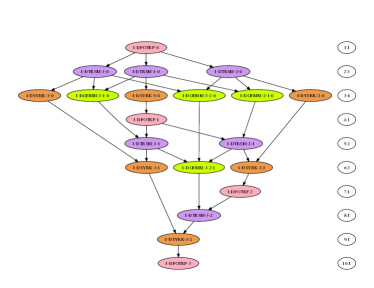
(a) Tasks perspective (equal weights)

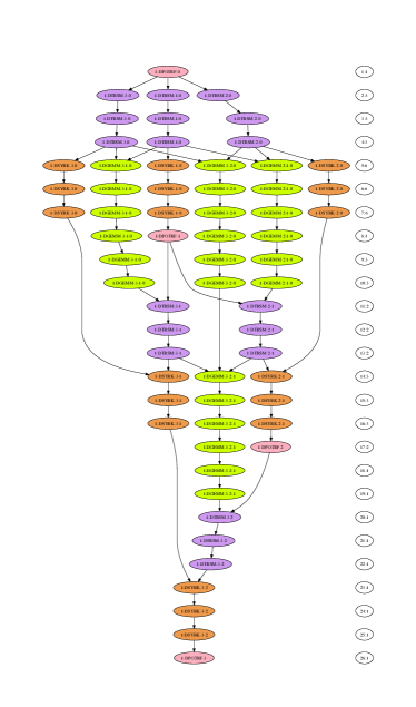
(b) Flops perspective (unequal weights)

Figure 1: TILE_POTRF DAGs for tasks and flops ($t=4$).

3 Analysis of Triangular matrix multiplication - TILE_LAUUM

As with the first step, the third step can have multiple variants dependent upon the order the result computed, either column or row wise, but the resulting DAGs are all identical (Figure 2(a)); it is simply a multiplication of two triangular matrices. However, since the result is stored in-place, there are many dependencies arising from a write-after-read (WAR) operation. In order to break this dependence, a buffer must be used to allow multiple operations to read a particular tile while another operation over writes it; we call the variants without buffer ‘in-place’ and those using buffers ‘out-of-place’. In so doing, the DAG changes dramatically as shown in Figure 2(a) and Figure 2(c). The cost of using the buffer is considered as one unit (whether we are flops-based or tasks-based) and is incorporated into the DAG. In either case, the lengths of the critical paths for both tasks-based and flops-based is linear in $t$ (Table 3).

For the in-place variants, the critical path for the unweighted tasks follows LAUUM, SYRK, TRSM for $t-1$ with a final LAUMM at the end such that the length in terms of $t$ becomes:

$$(1+1+1)(t-1)+1=3t-2$$

and for the weighted tasks the critical path follows LAUUM, SYRK with TRSM and GEMM for $t-2$, and TRSM and LAUUM bringing up the end:

$$1+3+(3+6)(t-2)+3+1=9t-10.$$

For the out-of-place condition, we have for the unweighted tasks a critical path of LAUUM followed by $t-1$ SYRKs and the cost of using the buffer:

$$1+(t-1)+1=t+1.$$

Observe that for the weighted tasks, the out-of-place critical path follows TRSM and $t-2$ GEMMs and the cost of using the buffer for values of $t\geq 3$ (for $t=2$, we would have $3t-1$):

$$3+6(t-2)+1=6t-8.$$

All of these are summarized in Table 3.

	Tasks	Flops
TILE_LAUUM (in-place)	$3t-2$	$9t-10$
TILE_LAUUM (out-of-place)	$t+1$	$6t-8$

Table 3: TILE_LAUUM critical path length ($t\geq 3$)

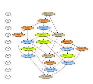
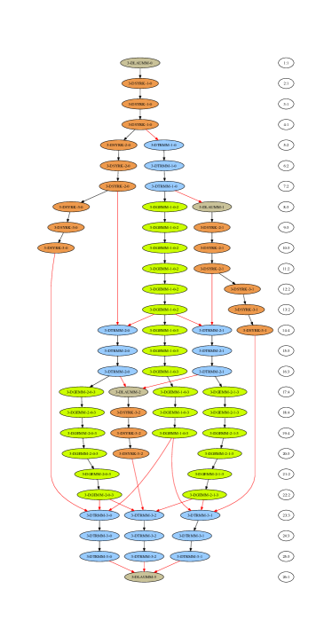
(a) Tasks perspective (equal weights, in-place)		(b) Flops perspective (unequal weights, in-place)
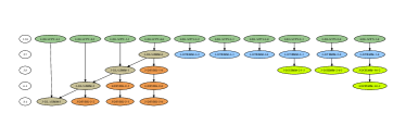
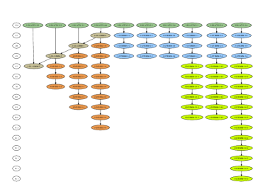
(c) Tasks perspective (equal weights, out-of-place)		(d) Flops perspective (unequal weights, out-of-place)

Figure 2: TILE_LAUUM DAGs for $t=4$, in-place and out-of-place.

4 Analysis of Triangular matrix inversion - TILE_TRTRI

Of the three steps, the triangular inversion provides the most interest. The six variants that we have studied can be grouped into two groups of three by consideration of the mathematical approach, either by using the left inverse $T^{-1}T=I$ or the right inverse $TT^{-1}=I$; variants 1 through 3 use the left inverse and 4 through 6 use the right inverse. The left inverse moves through the matrix from the upper left corner to the lower right and vice versa for the right inverse. Thus, when speaking of the DAGs and critical paths, we will focus on one group since the other group is similar. As with the triangular matrix multiplication, we consider both in-place variants and out-of-place variants, which break the some of the WAR dependencies.

Unlike in the previous sections, the DAGs for the three variants, for both in-place and out-of-place, are not identical as can be seen in tasks viewpoint in Figures 3 and 4.

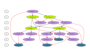
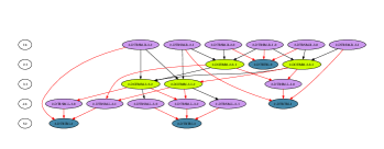
(b) TILE_TRTRI v2		(c) TILE_TRTRI v3

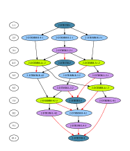
(a) TILE_TRTRI v1

Figure 3: DAGs for three variants of TILE_TRTRI ($t=4$) in-place.

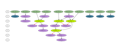
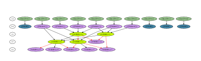
(b) TILE_TRTRI v2		(c) TILE_TRTRI v3

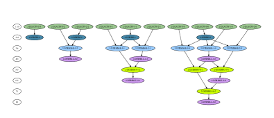
(a) TILE_TRTRI v1

Figure 4: DAGs for three variants of TILE_TRTRI ($t=4$) out-of-place.

As before, the lengths of the critical paths for the tasks and the flops are linear function of $t$ and are provided in Table 4. Note that although the in-place and out-of-place DAGs are different for a single variant, only variant 1 reaps any benefit from the use of the buffers. For the others, the cost of providing the buffer, which is considered to be one unit, negates any advantage it may provide.

In the unweighted case, we look at the lengths of the critical paths for the tasks. For variant 1, the critical path traverses $t-1$ TRTRI, TRMM and TRSMs ending with TRTRI. Thus

$$(1+1+1)(t-1)+1=3t-2.$$

For variant 2, the critical path traverses TRTRI followed by $t-2$ GEMM and TRSMs and ends with a TRSM and a TRTRI. Thus

$$1+(1+1)(t-2)+1+1=2t-1.$$

For variant 3, the critical path traverses TRTRI followed by $t-2$ GEMMs and ends with a TRSM and a TRTRI. Thus

$$1+(t-2)+1+1=t+1.$$

Similarly, in the weighted case we consider the critical path of each variant. For variant 1, the critical path traverses TRTRI followed by $t-2$ TRMM, TRSM and GEMMs and ends with a TRMM, TRSM and a TRTRI. Thus

$$1+(3+3+6)(t-2)+3+3+1=12t-16.$$

For variant 2, the critical path traverses TRTRI, followed by $t-2$ GEMM and TRSMs ending with a TRSM and TRTRI. Thus

$$3+(6+3)(t-2)+3+1=9t-11.$$

For variant 3, the critical path traverses TRTRI followed by $t-2$ GEMMs and ends with a TRSM and a TRTRI. Thus

$$3+6(t-2)+3+1=6t-5.$$

All of the above results are summarized in Table 4.

	Variant	Tasks	Flops
TRTRI (in-place)	1,4	$3t-2$	$12t-16$
	2,5	$2t-1$	$9t-11$
	3,6	$t+1$	$6t-5$
TRTRI (out-of-place)	1,4	$2t$	$9t-10$
	2,5	$2t-1$	$9t-11$
	3,6	$t+1$	$6t-5$

Table 4: TRTRI critical path length

5 Analysis of Cholesky inversion - CHOLINV

By combining the above three steps, we are able to compute the inverse of an SPD matrix. One approach is to perform the steps in sequential order such that each step is not started until the previous step has been completed fully. However, more parallelism can be obtained by interleaving the above three steps while still adhering to any dependencies that exist among tasks either within the step or between the steps and being cognizant of which variants are chosen to maximize the interleaving.

If one naively combines any variant of the TILE_POTRF with variants 4 through 6 of TILE_TRTRI, due to the fact that TILE_POTRF moves from upper left to lower right and these variants of TILE_TRTRI move from lower right to upper left, a sequential algorithm in terms of the steps is obtained. Furthermore, combining this with any of the variants of TILE_LAUUM would result in a completely sequential algorithm for the Cholesky inversion. We will see that indeed variants 1 through 3 for the TILE_TRTRI provide better theoretical and experimental results as we would expect.

For each of the interleaved variants, we continue to observe the linear behavior of the critical path in terms of tasks and flops as seen in Table 5. Of particular interest is that the combination with variant 1 of TILE_TRTRI leads to a critical path length, in terms of tasks, of four more tasks for the entire inversion ($3t+2$) as compared to just the Cholesky factorization ($3t-2$), independent of the number of tiles. This is quite a feat.

	Variant	Tasks	Flops
CHOLINV (in-place)	x1x	$3t+2$	$12t+2$
	x2x	$6t-1$	$18t-11$
	x3x	$3t+6$	$9t+23$
	x4x	$9t-6$	$30t-36$
	x5x	$8t-7$	$27t-34$
	x6x	$7t-3$	$24t-25$
CHOLINV (out-of-place)	x1x	$3t+2$	$9t+1$
	x2x	$3t+2$	$9t+7$
	x3x	$3t+3$	$9t+11$
	x4x	$5t$	$18t-14$
	x5x	$5t-3$	$18t-19$
	x6x	$5t-2$	$21t-24$

Table 5: CHOLINV critical path length

Depicted in Figure 5 is the Cholesky inversion, for four tiles, using variant 1 of TILE_TRTRI. Each step is identified by a different color to clearly see how the three steps are interleaving with each other. This combination of variants allows portions of TILE_TRTRI to start very early on within Step 1 as well as portions of TILE_LAUUM. One can observe the large amount of parallelism obtained by the interleaving of the three steps. We see that the whole Cholesky inversion as three times more tasks as the Cholesky factorization but finishes only 4 steps after.

With variant 3 of TILE_TRTRI, the flops-based critical path for the Cholesky inversion is the shortest. It is $9t+23$ which is only $33\frac{b^{3}}{3}$ flops more than the Cholesky factorization ($9t-10$). The difference between factorization and inversion is a constant number independent of the number of tiles. Once more, this is quite a feat. These observations are in complete contrast with an analysis based on the total number of flops. The total number of flops for Cholesky inversion is three times more than the Cholesky factorization. The tasks-based critical path lengths (using the appropriate variants) are about the same.

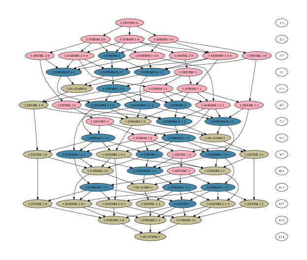
Figure 5: DAG for CHOLINV using variant 1 of TILE_TRTRI ($t=4$) in-place.

6 Application of critical path analysis. Upper bound on performances.

Having a closed form equation for the length of the critical path and knowing the total number of flops for the entire algorithm, we can provide a lower bound on the time to solution with the following reasoning: the total execution time is at least the number of the flops on the critical path times the flop rate ($\gamma$, in sec per flops), and it is at least the total number of flops divided by the number of processors times the flop rate. This lower bound on the execution time gives us an upper bound, $U(p)$, on the maximum performance with $p$ cores. We obtain

$$U(p)=\frac{1}{\gamma}\cdot\frac{\mbox{total number of flops}}{\max(\mbox{flops-based critical path length},\frac{\mbox{total number of flops}}{p})}.$$

So that

$$U(p)=\frac{1}{\gamma}\cdot\min(p,\frac{\mbox{total number of flops}}{\mbox{flops-based critical path length}}).$$

7 Experimental validation

Our experiments were performed on an AMD Istanbul machine. This is a 48-core machine which is composed of eight hexa-core Opteron 8439 SE (codename Istanbul) processors running at 2.8 GHz. Each core has a theoretical peak of 11.2 Gflop/s with a peak of 537.6 Gflop/s for the whole machine. The Istanbul micro-architecture is a NUMA architecture. Each socket has 6 MB of level-3 cache. Each processor has a 512 KB level-2 cache and a 128 KB level-1 cache. After having benchmarked the AMD ACML and Intel MKL BLAS libraries, we selected MKL (10.2) since it appeared to be slightly faster in our experimental context. Linux 2.6.32 and Intel Compilers 11.1 were also used.

The sequential performance is taken as: 6.43 Gflop/s. This is obtained by looking at a run on five or more cores and looking at the best achieved performance of the kernels in this configuration. Each core is able to perform 11.2 Gflop/s, so we estimate that our kernels are running at 57% of the peak.

In Figure 6, the performance of three variants for TILE_TRTRI are compared keeping the problem size and tile size fixed while increasing the number of threads. Variant 3 outperforms the other two which is in keeping with the analysis in Section 4 where the length of the critical path for Variant 3 is shorter than that of the others. Moreover, Variant 2 outperforms Variant 1 as was the case with the critical path lengths. Also note that our upper bounds on performance obtained in Section 6 (plain curves) are reasonably tight.

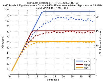
(a) TILE_TRTRI inplace

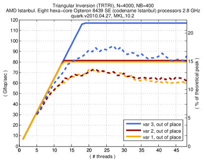
(b) TILE_TRTRI outofplace

Figure 6: Performance comparison of TILE_TRTRI for in-place and out-of-place. Dashed curves represent experimental data, plain curves represent the upper bounds derived in Section 6. See Table 4 for the critical path lengths of these variants.

Considering that the out-of-place variants did introduce some added overhead due to the necessity of the buffers, of note is the performance gains seen in Figure 6(b) for Variant 1 of TILE_TRTRI as compared to the decrease in performance of the other two variants. In Table 4, it is seen that the added buffers did not shorten the critical path for Variants 2 or 3, but did improve the critical path for Variant 1 as is reflected in the numerical experiments.

Figure 7 provides a comparison of all six variants where again the matrix size and the tile size are kept constant but the number of threads are increasing. This figure clearly mimics the information of Table 5 relative to the number of flops on the critical path lending credence to the criteria that a better variant has a shorter critical path.

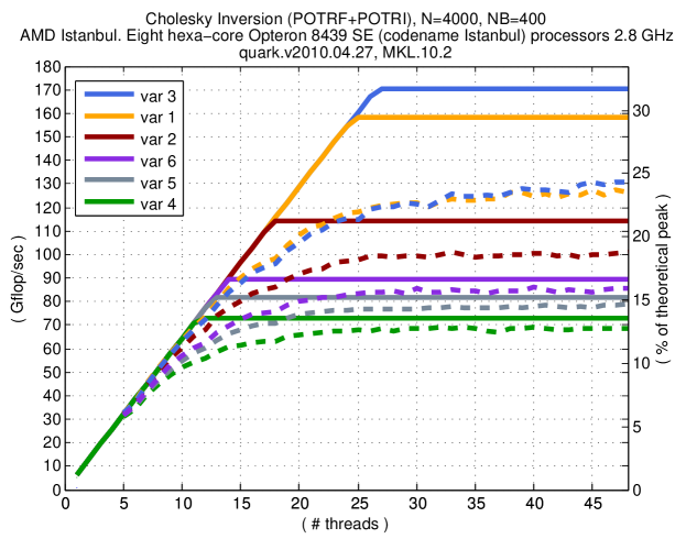
Figure 7: Performance of CHOLINV (in-place). Dashed curves represent experimental data, plain curves represent the upper bounds derived in Section 6. See Table 5 for the critical path lengths of these variants.

In order to provide a complete assessment, Figure 8 demonstrates a comparison of the complete Cholesky inversion using the dynamic scheduler quark v2010.04.27 against libflame r3935, MKL v10.2, LAPACK.3.2.1, and ScaLAPACK v1.8.0. In this experiment, the number of threads is held constant at 48, the tile size remains 200, and the matrix size varies. Once again, Variant 3 (quark331) shows improvement over Variant 1 (quark312). Variant 3 has the shortest flops-based critical path length.

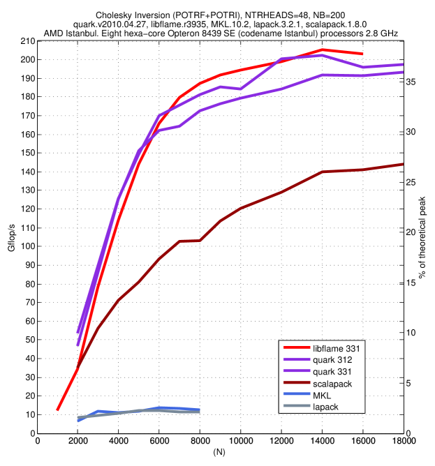
Figure 8: Performance comparison of LAPACK, MKL, ScaLAPACK, libflame and quark.

8 Conclusion

This paper continues our research on an effective implementation of tiled Cholesky inversion on multicore platforms [6]. Previous research [3, 5] presented algorithms and performances. In this manuscript, we explain that different algorithmic variants of the Cholesky inversion algorithm have different critical path lengths. We provide critical path lengths in terms of the number of tasks and in terms of the number of flops for all known variants, in place and out of place. This enables us to understand the scalability of each variant.

With the current trend in architecture towards multicore, the perspective of previous algorithms with a focus on the number of flops is now an antiquated metric. As more processors are made available, the length of the critical path becomes the limiting factor and less attention is spent on the total number of flops. Our intent is to introduce the length of the critical path as a better metric for an algorithm.

With this metric we understand why out of the six variants possible for TILE_TRTRI, Variant 3 is the most appropriate in the context of Cholesky inversion: Variant 3 is the one that provides the shortest flops-based critical path length in this context.

We validate the usefulness of our results with our software on a 48-core machine and present experimental comparison with LAPACK, ScaLAPACK, MKL, and libflame. We note that the Cholesky inversion software from this article will be released in the PLASMA release for SC 2010.

This manuscript focus on parallelism only and neglects (intentionally) any data transfer issues. This is the reason why the granularity of the problem has been kept constant all along. A better understanding of the performance of our algorithms needs to take into account a data transfer model. This is in our future work.

When there are few processors or when there is a large number of processors, our experimental data is often tight with our upper bound on performance. In between, the discrepancy between our upper bound and the experimental data can be larger and our future work also aims at reducing this discrepancy.

References

- [1] A. Buttari, J. Langou, J. Kurzak, J. Dongarra, Parallel tiled QR factorization for multicore architectures, Concurrency Computat.: Pract. Exper. 20 (13) (2008) 1573–1590.
- [2] A. Buttari, J. Langou, J. Kurzak, J. Dongarra, A class of parallel tiled linear algebra algorithms for multicore architectures., Parallel Computing 35 (1) (2009) 38–53.
- [3] G. Quintana-Ortí, E. S. Quintana-Ortí, R. A. van de Geijn, F. G. V. Zee, E. Chan, Programming matrix algorithms-by-blocks for thread-level parallelism, ACM Transactions on Mathematical Software 36 (3).
- [4] E. Agullo, J. Dongarra, B. Hadri, J. Kurzak, J. Langou, J. Langou, H. Ltaief, PLASMA Users’ Guide, Tech. rep., ICL, UTK (2009).
- [5] P. Bientinesi, B. Gunter, R. van de Geijn, Families of algorithms related to the inversion of a symmetric positive definite matrix, ACM Trans. Math. Softw. 35 (1) (2008) 1–22. doi:http://doi.acm.org/10.1145/1377603.1377606.
- [6] E. Agullo, H. Bouwmeester, J. Dongarra, J. Kurzak, J. Langou, L. Rosenberg, Towards an efficient tile matrix inversion of symmetric positive definite matrices on multicore architectures, in: VECPAR’10. 9th International Meeting High Performance Computing for Computational Science. Berkeley, CA (USA), June 22-25, 2010.