Ultrafast control of inelastic tunneling in a double semiconductor quantum well

Abstract

In a semiconductor-based double quantum well (QW) coupled to a degree of freedom with an internal dynamics, we demonstrate that the electronic motion is controllable within femtoseconds by applying appropriately shaped electromagnetic pulses. In particular, we consider a pulse-driven Al_xGa_1-xAs based symmetric double QW coupled to uniformly distributed or localized vibrational modes and present analytical results for the lowest two levels. These predictions are assessed and generalized by full-fledged numerical simulations showing that localization and time-stabilization of the driven electron dynamics is indeed possible under the conditions identified here, even with a simultaneous excitations of vibrational modes.

The impressive advance in fabrication, characterization and control of nano-scale systems handbook has fueled wide-ranged studies on the fundamental behavior of quantum systems and their utilization for practical applications, e.g. as elements in nano-circuits nanocirc , nano-oscillators nanoosc , nano-magnets nanomag and opto-electronic devices handbook . A similar rapid progress was also achieved in optics. Light sources are currently available in a wide range of intensity, duration and pulse shapes handbook_optics , offering new possibilities for the temporal and local manipulations of electronic properties of nanostructures. A paradigm example has been the ultrafast control of quantum states in a double-well (DW) structure which is of relevance for quantum computing application dwp . In this respect, three aspects are important: i) the swift electron localization in one of the wells starting from an arbitrary initial state, ii) maintaining this localization for a desired time, and iii) switching of the localization between the two wells. From a practical point of view, it is also essential to address the role of the coupling to the environment. In this work we study the electron dynamics in a typical Al_xGa_1-xAs-based QW coupled to vibrational modes with the aim of controlling and sustaining the electron motion on a femtosecond time scale via electromagnetic pulses. The DW potential barrier $V_{conf}(x)$ with a well separation $x_{0}$ confines the conduction electrons in the $x$-direction and is well modelled by $V_{conf}(x)=16~{}(V_{B}/x_{0}^{4})\left(x^{2}-x_{0}^{2}/4\right)^{2}$. Typical values for this system are $V_{B}\approx 240$ meV and $x_{0}\approx 10$ nm. The effective mass is assumed constant across the structure $m\approx 0.066m_{e}$ (as for GaAs, and $m_{e}$ is the free electron mass). The tunnel splitting $\hbar\Omega=E_{2}-E_{1}$ where $E_{1}$ and $E_{2}$ are the two lowest eigenenergies, is smaller than the separation from the third excited state, hence a consideration within a two level system (TLS) approximation is useful for low excitations and will be employed below for the analysis of qualitative trends. In addition we couple the electron dynamics to a degree of freedom ($y$) with an internal vibrational dynamics with the Hamiltonian $H_{R}=p_{y}^{2}/2m+ky^{2}/2$ and a coupling potential $H_{C}$. The full Hamiltonian reads then $H=H_{0}+H_{C}+H_{R}$. Here $H_{0}$ is the bare electron term; the coupling has the form $H_{C}=V_{0}(y/y_{0})\ v_{c}(x)$ with the function $v_{c}(x)$ describing the interaction strength along the structure, $y_{0}$ stands for the typical length scale associated with the oscillator potential. This problem resembles the rotational dynamics coupled to vibrations volker and also inelastic scanning tunneling experiments bringer . We will discuss two cases: (i) a uniform harmonic force acting on the electron, i.e. the coupling potential is $v_{c}(x)=x/x_{0}$, and (ii) a localized coupling $v_{c}(x)=\exp[-(x-x_{c})^{2}/2\lambda^{2}]$. Physically such vibrational (phononic) coupling may arise due to inelastic scattering of the tunneling electron in the DW, e.g. from pinned impurities that then vibrate around the minimum of the pinning potential.

A particularly efficient and swift mean for steering the electron dynamics in DW is the use of specially shaped femtosecond light pulses such as the so-called half cycle pulses (HCPs) hcp ; matoslocal . These are strongly asymmetric pulses with one short and strong half-cycle followed by a very weak and long half-cycle of opposite polarity. A key point in this control scheme is that the pulse duration has to be much shorter than the characteristic time of DW system ($T_{0}=2\pi/\Omega$) matoslocal . In this case, within the dipole approximation, the action of the pulses can be viewed effectively as impulsive kicks kick delivered at times $t_{k}$ with a strength $\Delta\mathbf{p}_{k}=\int\tilde{\mathbf{E}}_{k}dt$ where $\tilde{\mathbf{E}}_{k}$ is the electric field amplitude of the pulse and $t_{k}$ is the time when $\tilde{\mathbf{E}}_{k}$ reaches its peak, meaning that such a pulse sequence acts in effect as ${\mathbf{E}}_{k}=\Delta\mathbf{p}_{k}\delta(t-t_{k})$ and couples to the electron via $H_{L}(t)=xE(t)$ remark . This type of pulses can localize the electron within femtoseconds whereas the localization time for harmonic pulses is about few picoseconds bavli . How effective this scheme would remain if the tunneling electrons are coupled to an external degree of freedom is to be clarified here. Physically one would expect a similarly effective control scheme when the electron dynamics is coupled to an external bath as long as the time scales involved are longer than the pulse duration. However, the whole process is a coupled dynamical one with a non-trivial dependence on the properties of the external degree of freedom. We start thus from the two-level approximation. The case of zero vibrational coupling has been analyzed analytically matoslocal ; matosdoc . The electron in the ground state is completely delocalized across the heterostructure. In what follows we assume that in the ground state the electrons are decoupled from the vibrations. The vibrational coupling acts on the excited states, i.e. as soon as the external pulses are applied. Starting from this state, in order to localize the electron within the left well, it is sufficient to apply a single $\pi/2$-pulse in $x$-direction, i.e. $E(t)=\Delta p\ \delta(t)$ with $\alpha=2\mu\Delta p/\hbar=\pi/2$, where $\mu$ being the transition dipole between the first two states and $\alpha$ can be viewed as the ”pulse angle”. After acquiring an additional momentum shift $\Delta p$ the electron tunnels to the left well within the time $\tau_{L}=T_{0}/4$. As the system undergoes free Rabi-oscillations, the probability of finding the electron in the left well $P_{L}$ is given by $P_{L}(t)=\cos^{2}(\Omega t/2)$. Within the half-period of the Rabi oscillation the electron is then mainly localized in the right quantum well. To maintain the localization, one may kick periodically the electron back by an appropriate laser pulse. Applying the $\pi$-pulse ($\alpha=\pi$) to the free-evolving system at $t=t_{0}$ brings the system back to the localized state at $t=2t_{0}$ so that $P_{L}(0)=P_{L}(2t_{0})=1$. Therefore, the system has the periodicity $T$ of the array of laser pulses with $T=2t_{0}$. It is clear that the averaged localization will be higher if the interval $T$ between two consecutive pulses is shorter.

To proceed further, we map the electron Hamiltonian $H_{0}$ onto the spin-like TLS Hamiltonian $H_{TLS}=-\hbar\Omega\sigma_{z}/2$ (with $\sigma_{j}$ being the $j$ Pauli matrix). The mapping can be extended to incorporate the vibrational coupling by substituting the position operator with $-x_{0}\sigma_{x}/2$ (with eigenstates localized in the left, right potential minima). Applying this rule to the coupling term $v_{c}(x)$ leads to the so called spin-boson-model (see weiss and ref. therein). According to the theory of small polarons gitterman , the remaining vibrational degree of freedom $y$ is incorporated as a renormalization of the tunneling amplitude $\Omega\rightarrow\tilde{\Omega}=M_{n,n}\Omega$. Thus, the polaron transformation decouples the electron from the vibrational degrees of freedom, so that the remaining renormalized electron Hamiltonian can be handled analytically. We will use this model to make predictions for the modified control mechanism and compare with the full numerical exact result.

(i) Uniform coupling $v_{c}(x)=x/x_{0}$.

The effective electron Hamiltonian reduces to the simple form $\tilde{H}_{TLS}=-\hbar\tilde{\Omega}\sigma_{z}/2$ with the renormalized tunneling amplitude $\tilde{\Omega}$. For the ground state vibrations, the renormalization is given by the Franck-Condon factor $M_{0,0}=\exp[-V_{0}^{2}/(2\hbar^{2}\omega_{ph}^{2})]$. Thus, the effect of the vibrations is to slow down the electron dynamics. All control strategies remain unchanged, but the time for achieving an initial localization increases to $\tilde{\tau}_{L}=(\pi/2\Omega)\exp[V_{0}^{2}/(2\hbar^{2}\omega_{ph}^{2})]$. For an application of this model to the DW coupled to localized phonons, we may choose the Debye temperature as the maximum phonon energy, i.e. $\hbar\omega_{ph}=k_{B}\Theta$ adachi1 ; adachi2 , and measure the coupling constant $V_{0}$ in units of $\hbar\omega_{ph}$. In the phonon-free system, the characteristic time is $T_{0}\approx 80$ fs. Due to electron-phonon ($e\mathchar 45\relax ph$) coupling, it increases to $\tilde{T}_{0}\approx 110$ fs.

(ii) Localized coupling $v_{c}(x)=\exp[-(x-x_{c})^{2}/2\lambda^{2}]$.

Substituting again $x\rightarrow-x_{0}\sigma_{x}/2$, and evaluating the matrix exponent yields

$$H_{C}\rightarrow V_{0}\frac{y}{y_{0}}\exp\left[-\frac{x_{0}^{2}/4+x_{c}^{2}}{2\lambda^{2}}\right](\cosh\xi-\sigma_{x}\sinh\xi),\vspace{-0.1cm}$$ (1)

with $\xi=x_{0}x_{c}/2\lambda^{2}$. If the coupling to the phonon degree of freedom is centered around the potential barrier, i.e. $x_{c}=0$ and therefore $\sinh\xi=0$, $H_{C}$ will no longer depend on the electron term. The two degrees of freedom are then decoupled. For the full spectrum system, this means that the phonon effect plays a minor role because the wave function nearly vanishes at $x=0$.

The worst case scenario in terms of invalidating previous localization schemes is the $e\mathchar 45\relax ph$ interaction acting in one of the quantum wells, since the resulting problem has now the maximal asymmetry. For the TLS model (after the polaron transformation), this asymmetry leads to an additional term $H_{TLS}=-\hbar\tilde{\Omega}\sigma_{z}/2\mp\hbar\kappa\sigma_{x}/2$ for $x_{c}=\mp x_{0}/2$. The parameter $\kappa$ is quadratic in $V_{0}$: $\kappa=q(\lambda)V_{0}^{2}/\hbar^{2}\omega_{ph}$, where $q(\lambda)=1-e^{-x_{0}^{2}/2\lambda^{2}}$ is a prefactor describing the spatial extension of the $e\mathchar 45\relax ph$ interaction along the structure. For this situation we inferred the following results:
(a) Localizing the electron in the left well: Being no longer an eigenstate of the uncoupled Hamiltonian, the symmetric ground state of the DW potential oscillates and therefore gains the momentum $\mp\delta p_{1}$ for $x_{c}=\mp x_{0}/2$ and $t<T_{0}/4$. The corresponding pulse angle $\alpha$ must be modified according to $\alpha=\pi/2\mp\Delta\beta_{1}$ with $\Delta\beta_{1}=2\mu\delta p_{1}/\hbar$.
(b) Maintaining the localization: Due to the asymmetry, the electron tunnels back from the left well with an increased (a decreased) momentum $p\pm\delta p_{2}$ for $x_{c}=x_{0}/2$ ($x_{c}=-x_{0}/2$). Note that this additional momentum $\delta p_{2}$ depends on the time. In order to incorporate the dynamics arising from $\delta p_{2}$, the strategy is now to use the same pulse sequence, but to adjust the pulse angle to $\alpha=\pi\mp\Delta\beta_{2}$ with $\Delta\beta_{2}(t)=2\mu\delta p_{2}(t)/\hbar$.
The angles $\Delta\beta_{1}$ and $\Delta\beta_{2}$, or, equivalently the transferred momenta, can be calculated using the TLS model.
Alternatively, one can also compensate the asymmetric vibrational coupling by a constant electric field $E_{0}$ oriented in the $x$-direction. In the presence of the electric field $E^{(\pm)}_{0}=\mp\hbar\kappa/2\mu$, the TLS term proportional to $\sigma_{x}$ is exactly canceled. Thus, if the value $E^{(\pm)}_{0}$ is tuned appropriately, the control strategies remain the same as in the case of zero coupling.

In order to compare the optimal values obtained from the TLS model with the exact results, we performed a full numerical propagation based on the two-dimensional split-operator approach splitop . For definiteness we consider $x_{c}=-x_{0}/2$, the case $x_{c}=x_{0}/2$ can be treated analogously. For clarity we introduce the dimensionless coupling parameter $\gamma=2V_{0}/\hbar\omega_{ph}$. Our control quantity is the probability of finding the electron in the left well $P_{L}(t)$.

Localizing the electron in the left well

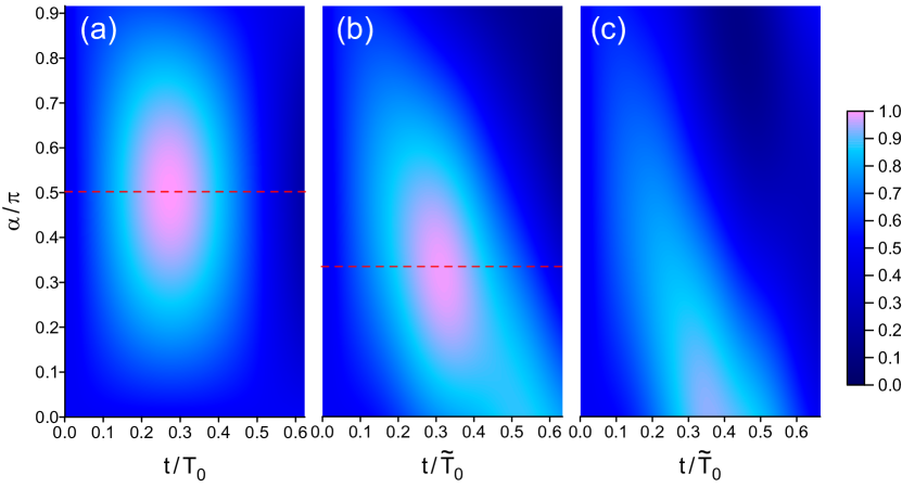
Figure 1: The time-dependent probability $P_{L}$ as a function of the applied laser pulse angle $\alpha=\frac{2\mu\Delta p}{\hbar}$ for different values of the rescaled coupling (a) $\gamma:=2V_{0}/\hbar\omega_{ph}=0$, (b) $\gamma=0.6$, and (c) $\gamma=1$.

In fig. (1), the time scale is given by the renormalized characteristic time $\tilde{T}_{0}$. The red dashed lines denote the optimal pulse angles obtained from the TLS model, which agrees well with the numerical result. In the case of full coupling fig. (1 c), an initial pulse

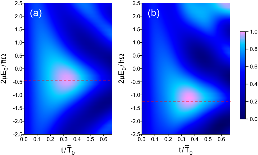
Figure 2: The time-dependent probability $P_{L}$, if additionally to the localizing laser pulse with $\alpha=\pi/2$ a constant electric field $E_{0}$ (measured in units of $2\mu/\hbar\Omega$) is applied, for different values of the coupling parameter: (a) $\gamma=0.6$, and (b) $\gamma=1$.

with any amplitude can not totally localize the electron, but $P_{L}$ still reaches values around 90%. In order to obtain full control over the electron in this scenario as well, one can use a constant electric field, as explained above. We apply the unmodified laser pulse with a pulse angle $\alpha=\pi/2$. Fig. (2) shows the effect on the dynamical localization. The constant electric field $E_{0}$ in fig. (2) is rescaled in units of $2\mu/\hbar\Omega$ so as to compare with $\kappa/\Omega$ (red dashed lines).

Maintaining the localization

If the electron has now been transferred predominantly to the left well, a periodic train of pulses with a pulse angle $\alpha=\pi-\Delta\beta_{2}$ for zero coupling leads to a very high degree of localization. Fig. (3) shows again the probability $P_{L}(t)$ but with the initial condition $P_{L}(t=0)=1$. Since the period of the pulses has been chosen as $T=80$ fs, $P_{L}$ shows a maximum for multiples of $T$, even in the case of a vibrational coupling. The red dashed lines represents the TLS results. Note that in fig. (3), the averaged localization is over 90 %.

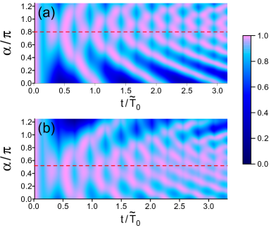
Figure 3: The time-dependent probability $P_{L}$ as a function of the pulse angle $\alpha$ of the train of laser pulses with the $T=80$ fs for values of the coupling parameter: (a) $\gamma=0.6$, and (b) $\gamma=1$.

Conclusions

We analyzed analytically and numerically the electron dynamics in a DW coupled to vibrational modes. Mapping onto a spin-model and using the polaron transformation we found analytical expressions for i) times and ii) light pulse parameters that are appropriate for switching the system from the initially delocalized to the localized target state and to maintain the localization. These estimates are in excellent agreement with the full-fledged two-dimensional numerical propagation. We considered two cases of uniform and localized vibrational coupling, and also when a static electric field is applied. Even in the presence of the vibrational environment we achieve an averaged localization of 90% which makes this system a suitable candidate for applications in quantum information or as an ultra-fast optical switch.

References

- (1) B. Bhushan, Springer Handbook of Nanotechnology (Ed.) 3rd ed., (2010, Springer, Berlin)
- (2) A. Alù and N. Engheta, Phys. Rev. Lett. 101, 043901 (2008)
- (3) S. B. Legoas, V. R. Coluci, S. F. Braga, P. Z. Coura, S. O. Dantas, and D. S. Galvão, Phys. Rev. Lett. 90, 055504 (2003)
- (4) H. Chik and J. M. Xu, Materials Science and Engineering R 43 103 (2004)
- (5) Handbook of Optics Vol. I-IV by Optical Society of America, McGraw-Hill, New York (2000)
- (6) J. Gorman, D. G. Hasko, and D. A. Williams, Phys. Rev. Lett. 95, 090502 (2005)
- (7) P. Marquetand, A. Materny, N. E. Henriksen, V. Engel, J. Chem. Phys. 120, 5871 (2004).
- (8) A. Bringer, J. Harris and J. W. Gadzuk, J. Phys.: Condens. Matter 5, 5141 (1993).
- (9) C. L. Stokely, F. B. Dunning, C. O. Reinhold, and A. K. Pattanayak, Phys. Rev. A 65, 021405 (2002)
- (10) A. Matos-Abiague, J. Berakdar, Appl. Phys. Lett. 84, 2346 (2004)
- (11) A. Bugacov, B. Piraux, M. Pont, R. Shakeshaft, Phys. Rev. A 51, 1490 (1995); 51, 4877 (1995); R. Robicheaux, Phys. Rev. A, 60, 431 (1999)
- (12) For numerical simulations we used HCP of shape and duration. Additional studies were made to clarify the role of tails of realistic HCPs on the electron dynamics. They confirm that our control scenarios are robust with respect to these effects.
- (13) R. Bavli, H. Metiu, Phys. Rev. Lett. 69, 1986 (1992)
- (14) A. Matos-Abiague, J. Berakdar, Phys. Rev. B 69, 155304 (2004); Europhys. Lett. 71, 705 (2005); Phys. Rev. A 73, 024102 (2006).
- (15) U.Weiss, Quantum Dissipative Systems, World Scientific, Singapore (2008)
- (16) M.I. Klinger, M. Gitterman, Phys. Rev. B 61, 3353 (2000)
- (17) S. Adachi, Physical Properties of III-V Semiconductor Compounds, Wiley, Weinheim (1992)
- (18) S. Adachi, GaAs and related materials: bulk semiconducting and superlattice properties, World Scientific, Singapore (1994)
- (19) T. K. Kjeldsen, Wave packet dynamics studied by ab initio methods: Applications to strong-field ionization of atoms and molecules, Ph. D. thesis (Department of Physics and Astronomy University of Århus, 2007)