Recurrence and Pólya number of general one-dimensional random walks

Abstract

The recurrence properties of random walks can be characterized by Pólya number, i.e., the probability that the walker has returned to the origin at least once. In this paper, we consider recurrence properties for a general 1D random walk on a line, in which at each time step the walker can move to the left or right with probabilities $l$ and $r$, or remain at the same position with probability $o$ ($l+r+o=1$). We calculate Pólya number $P$ of this model and find a simple expression for $P$ as, $P=1-\Delta$, where $\Delta$ is the absolute difference of $l$ and $r$ ($\Delta=|l-r|$). We prove this rigorous expression by the method of creative telescoping, and our result suggests that the walk is recurrent if and only if the left-moving probability $l$ equals to the right-moving probability $r$.

Random walk is related to the diffusion models and is a fundamental topic in discussions of Markov processes. Several properties of (classical) random walks, including dispersal distributions, first-passage times and encounter rates, have been extensively studied. The theory of random walk has been applied to computer science, physics, ecology, economics, and a number of other fields as a fundamental model for random processes in time rn1 ; rn2 ; rn3 ; rn4 .

An interesting question for random walks is whether the walker eventually returns to the starting point, which can be characterized by Pólya number, i.e., the probability that the walker has returned to the origin at least once during the time evolution. The concept of Pólya number was proposed by George Pólya, who is a mathematician and first discussed the recurrence property in classical random walks on infinite lattices in 1921 rn5 ; rn6 . Pólya pointed out if the number equals one, then the walk is called recurrent, otherwise the walk is transient because the walker has a nonzero probability to escape rn7 . As a consequence, Pólya showed that for one and two dimensional infinite lattices the walks are recurrent, while for three dimension or higher dimensions the walks are transient and a unique Pólya number is calculated for them rn8 . Recently, M. Štefaňák et al. extend the concept of Pólya number to characterize the recurrence properties of quantum walks rn9 ; rn10 ; rn11 . They point out that the recurrence behavior of quantum walks is not solely determined by the dimensionality of the structure, but also depend on the topology of the walk, choice of coin operators, and the initial coin state, etc rn9 ; rn10 ; rn11 . This suggests the Pólya number of random walks or quantum walks may depends on a variety of ingredients including the structural dimensionality and model parameters.

In this paper, we consider recurrence properties for a general one-dimensional random walk. The walk starts at $x=0$ on a line and at each time step the walker moves one unit towards the left or right with probabilities $l$ and $r$, or remain at the same position with probability $o$ ($l+r+o=1$). This general random walk model has some useful application in physical or chemical problems, and some of its dynamical properties requires a further study. Previous studies of one-dimensional random walk focus on the simple symmetric case where the walker moves to left and right with equal probability ($l=r=1/2$) rn10 . For instance, Pólya showed that the symmetric random walk is recurrent and its Pólya number equals to 1 rn12 ; rn13 . However, recurrence properties of this general random walk defined here are still unknown. As a consequence, we will calculate the Pólya number for this general random model and discuss its recurrence properties. We will try to derive an explicit expression for Pólya number, and reveal its dependence on the model parameters $l$, $r$ and $o$.

Pólya number of random walks can be expressed in terms of the return probability $p_{0}(t)$ rn12 ; rn10 , i.e., the probability for the walker returns to its original position $x=0$ at step $t$,

$$P=1-\frac{1}{\sum_{t=0}^{\infty}p_{0}(t)}.$$ (1)

Hence, the recurrence behavior of random walk is determined solely by the infinite summation of return probabilities. It is evident that if the summation of return probabilities diverges the walk is recurrent ($P=1$), and if the summation converges the walk is transient ($P<1$). To calculate the Pólya number, it is crucial to obtain the return probabilities. In the following, we will calculate the return probabilities for our general random walk model.

The return probability $p_{0}(t)$ can be obtained using the trinomial coefficients of $(l+o+r)^{t}$. Considering an ensemble of random walks after $t$ steps, in which the walker has $L$ steps moving left, $R$ steps moving right and $O$ steps remaining at the same position, then the probability for such random walks is $\frac{t!}{O!L!R!}o^{O}l^{L}r^{R}$ ($l+o+r=1$, $L+O+R=t$). Since the walker’s position $x$ is only dependant on the difference of right-moving steps $R$ and left-moving steps $L$, $x=R-L$, returning to the original position $x=0$ requires $R=L$. Therefore, the ensemble of random walks returning to $x=0$ involves sum over all possible $O$ subject to the constraints $R=L$ and $R+L+O=t$. Because $R+L$ is an even number, $t$ and $O$ must have the same parity. Here, we suppose $t=2n$, $O=2i$ for even $t$ and $O$, and $t=2n+1$, $O=2i+1$ for odd $t$ and $O$ ($i$ and $n$ are nonnegative integers, and $i\leq n$). We calculate the return probability for even $t$ and odd $t$ separately. For even $t$, the return probability is given by,

$$p_{0}(t)|_{t=2n}=\sum_{i=0}^{n}\frac{(2n)!}{(2i)!(n-i)!(n-i)!}o^{2i}l^{n-i}r^{n-i},$$ (2)

where $t=2n$, $O=2i$, $R=L=(t-O)/2=n-i$ are used in the above equation. Analogously, for odd $t$, the return probability is given by,

$$p_{0}(t)|_{t=2n+1}=\sum_{i=0}^{n}\frac{(2n+1)!}{(2i+1)!(n-i)!(n-i)!}o^{2i+1}l^{n-i}r^{n-i}.$$ (3)

The infinite summation of return probabilities $S$ can be determined by the sum of $p_{0}(2n)$ and $p_{0}(2n+1)$,

$$S=\sum_{t=0}^{\infty}p_{0}(t)=\sum_{n=0}^{\infty}\Big{(}p_{0}(t)|_{t=2n}+p_{0}(t)|_{t=2n+1}\Big{)}.$$ (4)

In order to get a simple expression for $S$, we define $\Delta=|r-l|$, thus $lr=\big{(}(1-o)^{2}-\Delta^{2}\big{)}/4$. Substituting this relation into Eq. (4), we get

$$\begin{array}[]{ll}S&=\displaystyle{\sum_{n=0}^{\infty}}\Big{(}p_{0}(t)|_{t=2n}+p_{0}(t)|_{t=2n+1}\Big{)}\\ &=\displaystyle{\sum_{n=0}^{\infty}}\Big{(}\sum_{i=0}^{n}\frac{(2n)!}{(2i)!(n-i)!(n-i)!}o^{2i}\big{(}\frac{(1-o)^{2}-\Delta^{2}}{4}\big{)}^{n-i}\\ &\ +\displaystyle{\sum_{i=0}^{n}}\frac{(2n+1)!}{(2i+1)!(n-i)!(n-i)!}o^{2i+1}\big{(}\frac{(1-o)^{2}-\Delta^{2}}{4}\big{)}^{n-i}\Big{)}\\ &=\displaystyle{\sum_{n=0}^{\infty}}\frac{(2n)!}{(n!)^{2}}\big{(}\frac{(1-o)^{2}-\Delta^{2}}{4}\big{)}^{n}\\ &\times\Big{(}\ _{2}F_{1}(-n,-n,1/2,\frac{o^{2}}{(1-o)^{2}-\Delta^{2}})+\\ &(2n+1)o\ _{2}F_{1}(-n,-n,3/2,\frac{o^{2}}{(1-o)^{2}-\Delta^{2}})\Big{)},\end{array}$$ (5)

where ${}_{2}F_{1}(a,b,c,z)$ is the Gauss Hypergeometric function. $S$ can be further simplified, for the sake of clarity, we first consider the case $o=0$. When $o=0$ the Hypergeometric function equals to 1, $S$ can be simplified as,

$$S=\sum_{n=0}^{\infty}\frac{(2n)!}{(n!)^{2}}\Big{(}\frac{1-\Delta^{2}}{4}\Big{)}^{n}=\frac{1}{\Delta}.$$ (6)

The last equality follows from the Taylor series expansion at $z=0$ for the function $1/\sqrt{1-4z}$.

For $o>0$, we find that $S$ also equals to $1/\Delta$. This result is surprising because $S$ does not depend on the remaining unmoving probability $o$. This suggests that, for all $o$ and $\Delta$, Eq. (5) can be simplified as,

$$S=\frac{1}{\Delta},\ \ \ \ \ \forall\ \ 0<o,\Delta\leq 1,o+\Delta\leq 1.$$ (7)

It is difficult to simplify Eq. (5) or prove Eq. (7) using the usual mathematical methods. Here, in the appendix, we prove this rigorous expression (7) by the method of creative telescoping. The method of creative telescoping rn14 ; rn15 ; rn16 is an algorithm to compute hypergeometric summation, definite integration, and prove combinatorial identity. Using this method, we transfer $S$ to the solution of a partial differential equation (See the proof in the appendix).

The Pólya number in Eq. (1) can be written as,

$$P=1-\frac{1}{S}=1-\Delta.$$ (8)

Consequently, we find a simple explicit expression for Pólya number, which is solely determined by the absolute difference of $l$ and $r$, $\Delta=|l-r|$.

According to Eq. (8), Pólya number $P$ equals to 1 for $\Delta=0$. This suggests that the walk is recurrent if and only if the left-moving probability $l$ equals to the right-moving probability $r$. Our result is consistent with previous conclusion that one-dimensional symmetric random walk ($l=r=1/2$) is recurrent. Our result also indicates that the infinite summation of return probabilities $S$ diverges for $\Delta=0$ and converges for $\Delta\neq 0$. To verify this point, we plot the return probability $p_{0}(t)$ as a function of step $t$ in Fig. 1. We find that $p_{0}(t)$ is a power-law decay as $p_{0}(t)\sim t^{-0.5}$ for $\Delta=0$ (See Fig. 1 (a) in the log-log plot) and exponential decay for $\Delta\neq 0$ (See Fig. 1 (b), (c) in the log-linear plot). Since $p_{0}(t)$ for $\Delta=0$ decays slower than $t^{-1}$ and decays faster than $t^{-1}$ for $\Delta\neq 0$, the infinite summation $S$ diverges for $\Delta=0$ and converges otherwise. Particularly, by means of Stirling’s approximation $n!\approx\sqrt{2\pi n}(n/e)^{n}$ for $o=0$, we find an asymptotic form for the return probability in Eq. (6): $p_{0}(t)\approx\sqrt{\frac{2}{\pi t}}(1-\Delta^{2})^{t/2}$ for even $t$ and $p_{0}(t)=0$ for odd $t$. For a certain value of $\Delta>0$, the decay behavior of $p_{0}(t)$ seems different for different values of $o$ (See Fig. 1 (b), (c)). However, the summations of $p_{0}(t)$ for different $o$ are identical and equal to $1/\Delta$. This result is some what unexpected and we provide a strict proof in the appendix.

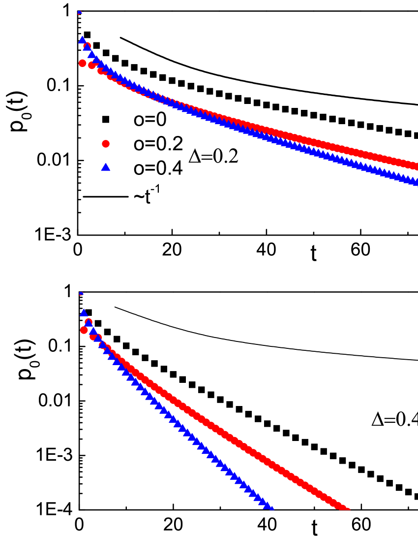
Figure 1: (Color online) Return probability $p_{0}(t)$ as a function of step $t$ for $\Delta=0$ (a), $\Delta=0.2$ (b) and $\Delta=0.4$ (c). For each value of $\Delta$, we plot $p_{0}(t)$ vs $t$ for $o=0$ (black squares), $o=0.2$ (red dots) and $o=0.4$ (blue triangles). The critical decay for convergence $p_{0}(t)\sim t^{-1}$ are also plotted in the figure. $p_{0}(t)$ shows a power-law decay $t^{-0.5}$ for $\Delta=0$ (See (a)), and $p_{0}(t)$ exhibits exponential decay for $\Delta>0$ (See (b) and (c)). It should be pointed out that for the case $o>0$, $p_{0}(t)$ is nonzero at all values of $t$, while $p_{0}(t)$ is zero at odd $t$ for $o=0$.

In summary, we have studied recurrence properties for a general 1D random walk on a line, in which at each time step the walker can move to the left or right with probabilities $l$ and $r$, or remain at the same position with probability $o$ ($l+r+o=1$). We calculate Pólya number $P$ of this model for the first time, and find a simple explicit expression for $P$ as, $P=1-\Delta$, where $\Delta$ is the absolute difference of $l$ and $r$ ($\Delta=|l-r|$). We prove this rigorous relation by the method of creative telescoping, and our result suggests that the walk is recurrent if and only if the left-moving probability $l$ equals to the right-moving probability $r$.

We thank Armin Straub and Dr. Koutschan for useful discussions. This work is supported by National Natural Science Foundation of China under project 10975057, the new Teacher Foundation of Soochow University under contracts Q3108908, Q4108910, and the extracurricular research foundation of undergraduates under project KY2010056A.

Appendix A The method of creative telescoping (MCT)

The method of creative telescoping, also known as Zeilberger’s algorithm rn14 ; rn15 ; rn16 , is a powerful tool for solving problem involving definite integration and summation of hypergeometric function. Suppose we are given a certain holonomic function of two variables $F(z,n)$ ($n\in Integers$, $z\in Reals$), and it is required to prove that the summation of $F(z,n)$ over $n$ equals to $f(z)$,

$$\sum_{n}F(z,n)=f(z).$$ (9)

The basic idea of creative telescoping algorithm is to find a linear recurrence equation for the summands $F(z,n)$. This could be done by constructing a differential operator $\hat{L}$ with coefficients being polynomials in $z$, and a new function $G(z,n)$ satisfying,

$$\hat{L}(z)F(z,n)=G(z,n+1)-G(z,n).$$ (10)

Thus $\hat{L}(z)$ operating on the summation $\sum_{n}F(z,n)$ is determined by the difference of upper bound and lower bound $G_{0}(z)=G(z,n_{max})-G(z,n_{min})$. Then we just need to check both sides of Eq. (9) satisfy recurrence equations: $\hat{L}(z)\sum_{n}F(z,n)=G_{0}(z)$, $\hat{L}(z)f(z)=G_{0}(z)$, and check Eq. (9) holds for some initial conditions.

Several algorithms for computing creative telescoping relations have been developed in the past rn17 . The main programs are Zeilberger’s Maple program and Mathematica program written by Peter Paule and Markus Schorn rn17 ; rn18 ; rn19 . Here, we use the mathematical program to compute the creative telescoping relation for our problem.

Appendix B Proof of $S=\frac{1}{\Delta}$ using MCT

In this section, we prove $S=\frac{1}{\Delta}$ using the method of creative telescoping (MCT). We use the Mathematica package Holonomic Functions rn17 ; rn20 ; rn21 to create a recurrence relation for the summands $s_{n}(o,\Delta)$ in Eq. (5),

$$\Big{(}2oD_{o}+\Delta D_{\Delta}+1+(S_{n}-1)\frac{1}{\Delta}D_{\Delta}\Big{)}s_{n}(o,\Delta)=0,$$ (11)

where $D_{o}$, $D_{\Delta}$ are the partial differential operator ($D_{o}\equiv\partial/\partial o$, $D_{\Delta}\equiv\partial/\partial\Delta$), $S_{n}$ is the shift operator satisfying $S_{n}f(n)=f(n+1)$.

Summing over $n$ leads to,

$$\Big{(}2oD_{o}+\Delta D_{\Delta}+1\Big{)}S+\displaystyle{\sum_{n=0}^{\infty}}(S_{n}-1)\frac{1}{\Delta}D_{\Delta}s_{n}(o,\Delta)=0.$$ (12)

The second term in the above equation is a telescoping series, the central terms are cancelled and only leave the last term and first term. Noting that $\frac{1}{\Delta}D_{\Delta}s_{n}(o,\Delta)$ are zero for $n=0$ and $n\rightarrow\infty$, the second term in Eq. (12) equals to $0$. Hence the infinite summation of return probabilities $S$ satisfies,

$$\Big{(}2oD_{o}+\Delta D_{\Delta}+1\Big{)}S=0.$$ (13)

It is easy to check $\frac{1}{\Delta}$ also satisfies the above partial differential equation. Combining with the initial condition $S=\frac{1}{\Delta}$ for $o=0$ (See Eq. (6)), $S=\frac{1}{\Delta}$ holds for all $o$ and $\Delta$.

References

- (1) N. Guillotin-Plantard and R. Schott, Dynamic Random Walks: Theory and Application (Elsevier, Amsterdam, 2006).
- (2) W. Woess, Random Walks on Infinite Graphs and Groups (Cambridge: Cambridge University Press, 2000).
- (3) F Spitzer, Principles of random walk(Springer, Berlin, 2000).
- (4) G. H. Weiss, Aspects and applications of the random walk, (North-Holland, New york, 1994).
- (5) G. Pólya, How to Solve It, (Princeton University Press, 1945).
- (6) G. L. Alexanderson, The Random Walks of George Pólya, (Mathematical Association of America, 2000).
-
(7)
W. E. Weisstein, Pólya’s Random Walk Constants, From MathWorld-A Wolfram Web Resource.
http://mathworld.wolfram.com/PolyasRandomWalkConstants.html - (8) S. R. Finch, Pólya’s Random Walk Constant, in §5.9 Mathematical Constants (Cambridge University Press, pp. 322-331, 2003).
- (9) M. Štefaňák, I. Jex and T. Kiss, Phys. Rev. Lett 100, 020501 (2008).
- (10) M. Štefaňák, T. Kiss and I. Jex, Phys. Rev. A 78, 032306 (2008).
- (11) Z. Darázs and T. Kiss, Phys. Rev. A 81, 062319 (2010).
- (12) C. Domb, On Multiple Returns in the Random-Walk Problem, Proc. Cambridge Philos. Soc. 50, 586-591 (1954).
- (13) E. W. Montroll, Random Walks in Multidimensional Spaces, Especially on Periodic Lattices, J. SIAM 4, 241-260 (1956).
- (14) D. Zeilberger, The Method of Creative Telescoping, J. Symbolic Computation 11, 195-204 (1991).
- (15) D. Zeilberger, A Holonomic Systems Approach to Special Function Identities, J. Comput. Appl. Math. 32, 321-368 (1990).
- (16) D. Zeilberger, A Fast Algorithm for Proving Terminating Hypergeometric Series Identities, Discrete Math. 80, 207-211 (1990).
- (17) M. Petkovšek, H. S. Wilf and D. Zeilberger, A=B, (AK Peters, Ltd. 1996)).
-
(18)
http://www.math.temple.edu/
~zeilberg/programs.html. - (19) P. Paule and M. Schorn, A Mathematica Version of Zeilberger’s Algorithm for Proving Binomial Coefficient Identities, J. Symbolic Comput. 20, pp. 673-698 (1995).
- (20) C. Koutschan, A Fast Approach to Creative Telescoping, arxiv:1004.3314
-
(21)
The Holonomic package can be downloaded at
http://www.risc.uni-linz.ac.at/research/combinat/software/