Asymptotic Orbits in Barred Spiral Galaxies

Abstract

We study the formation of the spiral structure of barred spiral galaxies, using an $N$-body model. The evolution of this $N$-body model in the adiabatic approximation maintains a strong spiral pattern for more than 10 bar rotations. We find that this longevity of the spiral arms is mainly due to the phenomenon of stickiness of chaotic orbits close to the unstable asymptotic manifolds originated from the main unstable periodic orbits, both inside and outside corotation. The stickiness along the manifolds corresponding to different energy levels supports parts of the spiral structure. The loci of the disc velocity minima (where the particles spend most of their time, in the configuration space) reveal the density maxima and therefore the main morphological structures of the system. We study the relation of these loci with those of the apocentres and pericentres at different energy levels. The diffusion of the sticky chaotic orbits outwards is slow and depends on the initial conditions and the corresponding Jacobi constant.

1 Introduction

Galactic dynamics together with celestial mechanics have played a leading role in the study of orbits as well as in the study of order and chaos. Many decades ago and for a long time the main interest was about regular orbits since they were considered as the main building blocks of galaxies. The main idea was that regular orbits are structurally robust and therefore they are able to support various morphological features. The most extreme manifestation was elliptical galaxies for which no chaotic orbits were considered to exist (de Zeeuw, 1985; Binney & Tremaine, 1987). In rotating galaxies the picture was more confused, especially after the study of the main periodic orbits in systems representing barred galaxies. These studies showed the existence of many unstable orbits (especially near corotation) which are generators of chaos (Contopoulos, 1981). Chaos was found in the 80’s near the ends of the bar (Sparke & Sellwood, 1987; Contopoulos & Grosbol, 1989). However, chaos was not considered as responsible for some of the main features of the galaxies like the spiral arms beyond corotation.

The importance of chaos was realized mainly in the 90’s, with application both in elliptical and in barred spiral galaxies, mostly in steady state cases (Merritt, 1996; Kaufmann & Contopoulos, 1996).

Only in the 2000’s people started to consider asymptotic orbits emanating from the unstable periodic orbits in explaining the main features of galaxies, like the spiral structure in barred spiral galaxies. The asymptotic orbits have initial conditions on the asymptotic manifolds of unstable periodic orbits. This study has been done either by using analytical potentials or by using $N$-body simulations (Voglis et al., 2006a; Contopoulos & Patsis, 2006; Romero-Gomez et al., 2006, 2007; , 2008; Athanassoula et al., 2009a; Harsoula & Kalapotharakos, 2009; Athanassoula et al., 2009b). The former method is not self consistent, but it has the advantage of the analytical form of the potential, allowing the free choice of all the parameters (like, for example, the strength of the bar and of the spiral perturbation, or the pattern speed of the bar). The latter method has the advantage of self consistency, but the time evolving potential and pattern speed imply a secular evolution of the system that makes the study harder.

Photometric data have shown that spiral structures are related to the old stellar disk (Grosbol et al., 2004). Analytical models and $N$-body dissipationless simulations have shown that, the chaotic domains are small in normal spiral galaxies (non barred), because the spiral perturbations are relatively small. Therefore, in many studies up to now it was argued that orbits near some stable periodic orbits (regular motions) can support the spiral pattern (see for example Lin & Shu, 1964; Kalnajs, 1971; Lynden-Bell & Kalnajs, 1972; Contopoulos, 1975; , 1977).

In Kaufmann & Contopoulos (1996) the authors pointed out the role of the so-called ‘hot population’ (Sparke & Sellwood, 1987), in supporting the inner parts of the spiral arms extending beyond the bar. They found chaotic orbits that wander stochastically, partly inside and partly outside corotation. In strong barred galaxies the chaotic domains of phase space have been proved very important (see for example Shen & Sellwood, 2004).

The role of the chaotic orbits in the spiral structure of a galaxy was pursued by Voglis et al. (2006b), using self-consistent $N$-body simulations of barred spiral galaxies, where they found long living spiral arms composed almost entirely of chaotic orbits.

Most chaotic orbits are connected to the asymptotic manifolds of the main unstable periodic orbits. Voglis et al. (2006a) and (2008) have considered the apocentric positions of the asymptotic orbits and the coalescence of all the unstable manifolds in a certain range of energy levels. On the other hand Romero-Gomez et al. (2006, 2007) and Athanassoula et al. (2009a, b) put the emphasis on the asymptotic manifolds emanating only from the unstable periodic orbits of families originating at the Lagrangian points $L_{1}$ and $L_{2}$.

In this paper we study a certain snapshot of a 3-D $N$-body simulation of a barred spiral galaxy, in order to give a more concrete and explicit description of the mechanism of construction of the spiral structure out of sticky chaotic orbits which are close to asymptotic orbits from various unstable periodic orbits. Since the $N$-body simulation is a self-consistent process, it gives all the details of the secular evolution of the galactic system during a Hubble time, having a potential and a pattern speed that vary with time. However by using frozen potentials and constant pattern speeds that correspond to certain snapshots of the evolution we are able to study the role of chaotic orbits in supporting a spiral structure that survives for more than 10 bar rotations, i.e. for at least 1/3 of the Hubble time. The sequence of these snapshots can be considered as an adiabatic approximation of the real galaxy evolution.

Chaotic orbits spend a long time close and along the unstable asymptotic manifolds of the unstable periodic orbits in the phase space, due to phenomena of stickiness (see Contopoulos & Harsoula, 2008). In our model, there are energy levels where the phase space is not bounded outwards and chaotic orbits can escape from the system. However, the escape rate is very small, due to stickiness. The orbits spend most of their time close to velocity minima on the rotation plane of the galaxy.

We show that the loci of velocity minima are connected with the maxima of the density distribution in the configuration space in every energy level and find the connection of these geometrical loci with the apocentres and the pericentres of the orbits.

We find the characteristic diagrams of the most important 3-D periodic families and we reveal the spiral structure of the galaxy by integrating chaotic orbits that lie close and along the main unstable periodic orbits. Finally, we construct the space configuration by superimposing orbits belonging to different energy levels. The space distribution of the apocentres and pericentres of these orbits is very similar to the apocentric and pericentric manifolds of 2-D asymptotic orbits having initial conditions along the unstable asymptotic curves of the 2D periodic orbits.

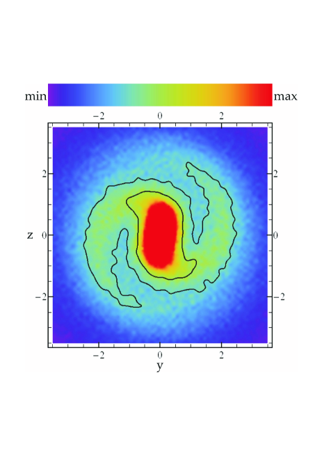
Figure 1: The density distribution (in the color scale indicated in the top of the panel) of the projected particles of our model on the rotation $y-z$ plane made by the superposition of 20 snapshots corresponding to the first 20$T_{hmct}$ of the integration of the system in the fixed effective potential. Black curves denote characteristic density contours revealing the spiral structure. Note that the color bar shown in this figure applies for all the color scales used in the following figures.

The paper is organized as follows: In section 2 we give a description of the system providing its main properties. We make a frequency analysis separately for the chaotic and regular populations. In section 3 we discuss the role of the apocentres and the pericentres of the orbits in comparison with the loci of the minimum velocities on the rotation plane. In section 4 we discuss the role of the sticky resonant orbits in supporting the spiral structure of the system. We present examples of specific periodic orbits that are able to reconstruct the main features of the galaxy. Moreover, we discuss the role of the apocentric and pericentric intersections of the 2D asymptotic orbits. In section 5 we give a description of the way the orbits escape from the system and finally in section 6 we present our conclusions.

2 Description of the model

The initial conditions of our $N$-body model, were created by Voglis et al. (2006b) where four experiments with different pattern speeds simulating barred spiral galaxies were produced. In our paper we use the $QR4$ model of Voglis et al. (2006b) (the experiment with the greatest value of the bar’s pattern speed).

We use $1.5\times 10^{5}$ particles in our simulation. The time unit is taken equal to the half mass crossing time of the system (hereafter $T_{hmct}$). A Hubble time corresponds to about $300T_{hmct}$. The length unit is taken equal to the half mass radius of the system (hereafter $r_{hm}$). Finally, the plane of rotation is the $y-z$ plane (intermediate-long axes) and the sense of rotation is clockwise.

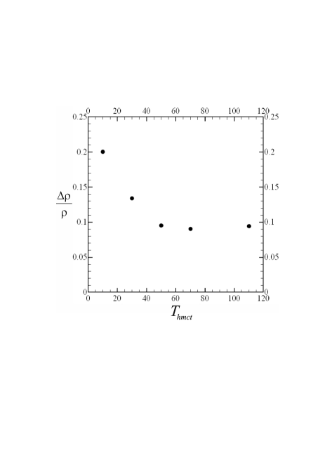
Figure 2: The time evolution of the amplitude of the spiral perturbation $\delta\rho/\rho$ at $r\approx 1.7r_{hm}$. We observe that the spiral structure fades out gradually.

The Jacobi constant $E_{j}$ of an orbit is given by the relation

$$E_{j}=\frac{1}{2}(\dot{x}^{2}+\dot{y}^{2}+\dot{z}^{2})+V(x,y,z)-\frac{1}{2}\Omega_{p}^{2}R_{yz}^{2}$$ (1)

where $V(x,y,z)$ is the full 3D ‘frozen’ potential, given by a Smooth Field Code (SFC code) as an expansion of a bi-orthogonal basis set, $\dot{x},\dot{y},\dot{z}$ are the velocities in the rotating frame of reference and $\Omega_{p}$ is the angular velocity of the bar (or pattern speed) at the studied snapshot. The value $R_{yz}$ is the distance from the rotation axis $\left(\sqrt{y^{2}+z^{2}}\right)$. The Jacobi constant $E_{j}$ is called also “energy in the rotating frame” and can be written as

$$E_{j}=\frac{1}{2}(\dot{x}^{2}+\dot{y}^{2}+\dot{z}^{2})+V_{eff}(x,y,z)$$ (2)

where $V_{eff}(x,y,z)=V(x,y,z)-\frac{1}{2}\Omega_{p}^{2}R_{yz}^{2}$ is the effective potential.

The energy of the orbit in the inertial frame is related to the Jacobi constant by the following relation

$$E=E_{j}+\mathbf{\Omega_{p}}\cdot\mathbf{L}$$ (3)

where $\mathbf{L}$ is the angular momentum in the inertial frame of reference and $\mathbf{\Omega_{p}}=-\Omega_{p}\mathbf{i}$, $\mathbf{i}$ being the unit vector along the $x$-axis. Therefore the inertial energy reads

$$E=E_{j}-\Omega_{p}(yP_{z}-zP_{y})$$ (4)

where $P_{y},P_{z}$ are the momenta in the inertial frame of reference. Since

$$P_{y}=\dot{y}+\Omega_{p}z,~{}~{}~{}~{}~{}~{}P_{z}=\dot{z}-\Omega_{p}y$$ (5)

we have

$$E=\frac{1}{2}(\dot{x}^{2}+\dot{y}^{2}+\dot{z}^{2})-\Omega_{p}(\dot{z}y-\dot{y}z)+V(x,y,z)+\frac{1}{2}\Omega_{p}^{2}R^{2}_{yz}$$ (6)

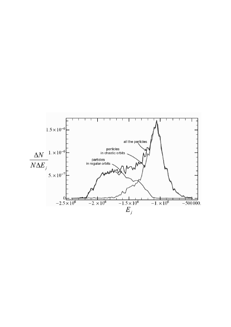
Figure 3: The distribution of the Jacobi constant values for all the particles, for the particles moving in regular orbits and for the particles moving in chaotic orbits. The maximum of the distribution corresponds to chaotic particles around corotation.

Our study is made in a distinct snapshot of the $N$-body simulation that corresponds to 55$T_{hmct}$. At this snapshot the spiral structure of the galaxy is clearly visible and moreover it survives for several rotations of the bar. In order to study the mechanism that creates this spiral structure which lasts for such a long time we fix the potential and the pattern speed and we study the role of chaotic orbits in this fixed potential. The corresponding value of the pattern speed is $\Omega_{p}\approx 2\pi/8T_{hmct}$ and is calculated in Voglis et al. (2006b) (see Fig. 4a of that paper). In real units this value corresponds to $\approx 25km~{}sec^{-1}~{}kpc^{-1}$. This value is in the range of the values observed in late type barred spiral galaxies (see for example Fathi et al., 2009).

By integrating all the orbits in this fixed effective potential we reveal the longevity of the spiral structure for at least $100T_{hmct}$, while after much longer times this structure disappears.

In Fig. 1 we plot, on the rotation plane $y-z$, the superposition of 20 snapshots corresponding to the first $20T_{hmct}$ of the integration time of the system in the fixed effective potential. Such a superposition consists of more than $2.5\times 10^{6}$ particles and allows us to reduce significantly the noise that appears when the number of particles is small. Since the density is now clearly defined, we can safely quantify the spiral perturbation. In Fig. 2 we show the time evolution of the amplitude of the spiral perturbation in our model. More precisely, we plot the density excess ($\delta\rho/\rho$) caused by the spiral structure in a specific radius that corresponds to $\approx 1.7r_{hm}$ as a function of time. After a time period of $100T_{hmct}$, during which the bar has completed $\approx 13$ rotations, the spiral perturbation is still marginally detectable. This time corresponds to 1/3 of the Hubble time.

Figure 3 gives the distribution of the Jacobi constants (Eq. 2) for all the particles and separately for chaotic and for regular orbits. The distinction between the two populations is done by the method introduced by Voglis et al. (2006b). The percentage of chaotic orbits is found to be $\approx 60\%$. The maximum of the distribution of the chaotic orbits is found between the values $E_{j}(L_{1})\approx-1120000$ and $E_{j}(L_{4})\approx-1080000$ corresponding to the Jacobi constant values of the Lagrangian points $L_{1,2}$ and $L_{4,5}$ respectively. From Fig. 3 it is obvious that the regular motions are restricted inside corotation and therefore they support the shape of the bar, while chaotic orbits are responsible for the spiral structure outside corotation.

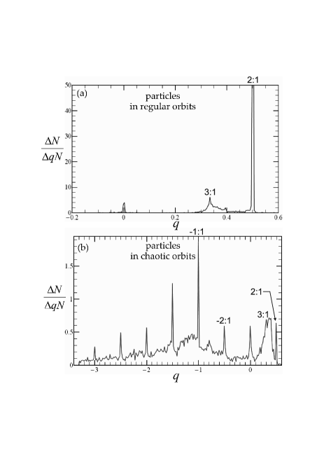
Figure 4: The frequency analysis of (a) the regular component and (b) the chaotic component of the system. The frequency ratio $q$ is given by Eq. (7). We see that the vast majority of regular orbits lie inside corotation $(q>0)$ (especially around 2:1 resonance) while the chaotic orbits lie both inside $(q>0)$ and outside corotation $(q<0)$. The various spikes shown in (b) correspond to chaotic orbits sticking close to various resonances.

Figure 4 presents the frequency analysis of the regular component (Fig. 4a) and of the chaotic component (Fig. 4b) of the system. We are only interested in revealing the “disc” resonances on the rotation plane and therefore the frequency analysis is made in the 2D projection of the orbits on the $y-z$ plane. However, there exist also vertical resonances that influence mainly the edge-on profiles of our systems (see Patsis et al., 2002).

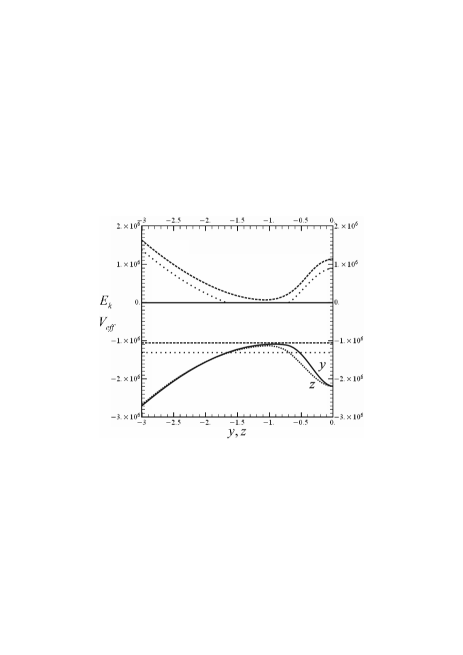
Figure 5: The effective potential $V_{eff}$ along the $y$-axis (black solid line) and along the $z$-axis (black dotted line). The two curves of kinetic energy $E_{k}$ (dotted and dashed curves) correspond to two different energy levels $E_{j}=-1300000<E_{j}(L_{1})$ (dotted line) and $E_{j}=-1050000>E_{j}(L_{1})$ (dashed line). In the former case the minimum velocity corresponds to apocentres for the motion inside corotation and to pericentres for the motion lying outside corotation. In the latter case the minimum velocity corresponds to the position of the maximum of $V_{eff}$.

The “frequency ratio” $q$ is a parameter given by the relation

$$q=\frac{\Omega-\Omega_{p}}{\kappa}$$ (7)

where $\Omega$ is the angular velocity of a particle in the inertial frame of reference and $\kappa$ is the epicyclic (radial) frequency (Binney & Tremaine, 1987). Positive $q$ values correspond to resonances inside corotation while negative $q$ values correspond to resonances outside corotation, which are related only to chaotic orbits. In Fig. 4a we see that the main resonance of the regular orbits (inside corotation) is the 2:1 resonance (or inner Lindblad resonance), while there is also a small number of particles around the 3:1 resonance and an even smaller number around corotation $(q=0)$. The vast majority of these orbits support the bar of the system. Figure 4b shows that a rather small percentage of chaotic orbits inside corotation lie near important resonances (e.g. 2:1, 3:1 and 4:1). These represent sticky chaotic orbits mainly supporting the outer layers of the bar (see Harsoula & Kalapotharakos, 2009) and the innermost parts of the spiral structure. The rest of the chaotic orbits move around corotation and outside it and some of them stick around specific resonances ($q$=0, -0.5, -1, -1.5, -2, -2.5, -3). The $q=0$ population corresponds to chaotic orbits located around corotation and close to the $PL_{1}$, $PL_{2}$, $PL_{4}$ and $PL_{5}$ families (nomenclature after Voglis et al., 2006a). Below we will show that the chaotic orbits sticking along the asymptotic manifolds originating from these unstable periodic orbits are responsible for the spiral structure of the system.

3 The role of the apocentres and pericentres

In this section we discuss the role of apocentres or pericentres in revealing the morphological features of the system and we relate their geometrical loci with the locus of the velocity minima on the rotation plane.

The distribution of the radial velocities $\dot{r}$ of the $N$-body orbits has a preferable concentration around the value zero, indicating that the apocentres and pericentres should play an important role for the system.

The geometrical loci of the minima of the velocities $v_{yz}$ on the rotation plane should correspond to the maxima of the density distribution on the configuration space, because particles spend most of their time there. It is of interest to investigate how these loci are related to the apocentres or the pericentres of the orbits.

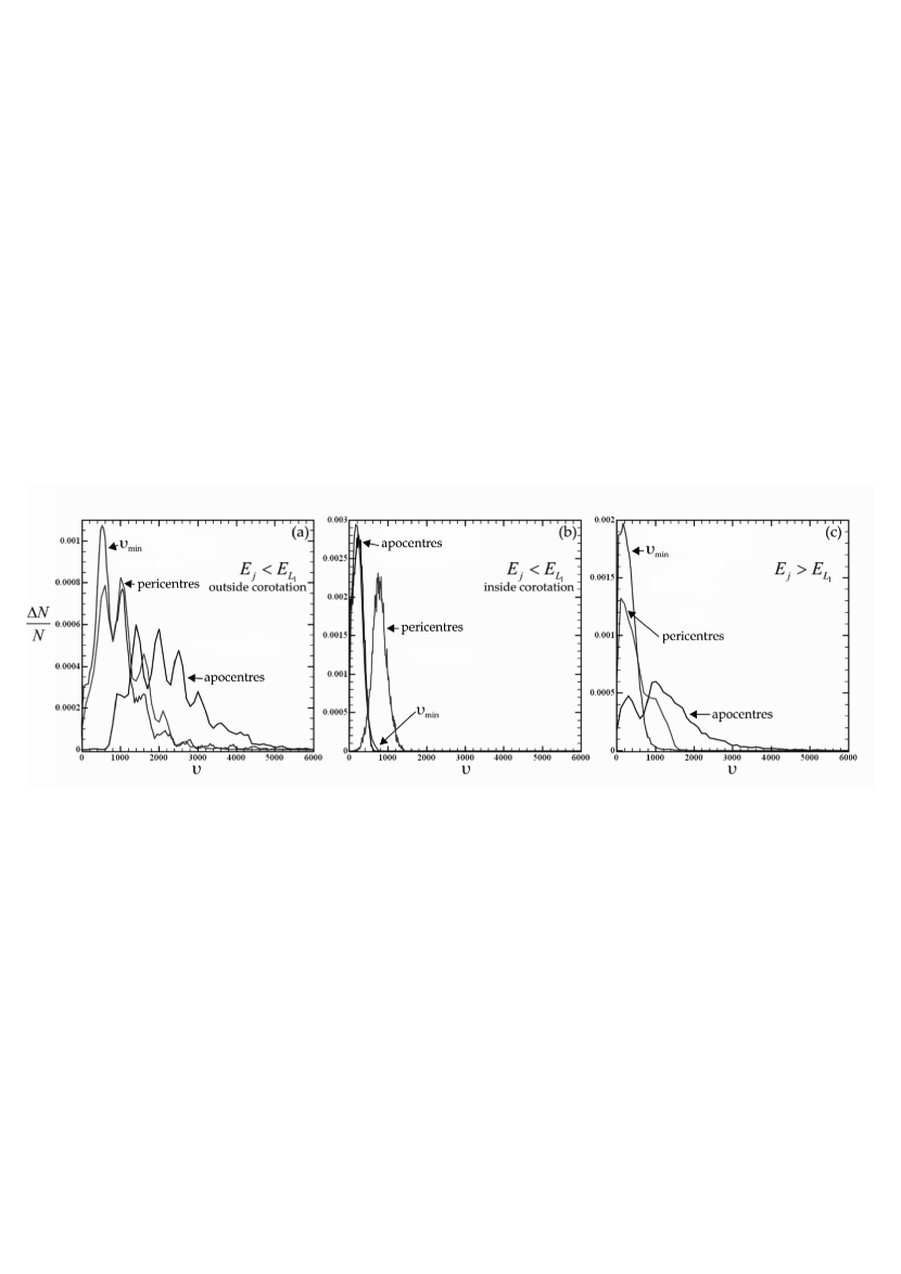
Figure 6: The distribution of the velocities of the apocentres, of the pericentres and of the velocity minima for (a) $E_{j}<E_{j}(L_{1})$ outside corotation (b) $E_{j}<E_{j}(L_{1})$ inside corotation and (c) for $E_{j}>E_{j}(L_{1})$ where the areas inside and outside corotation can communicate.

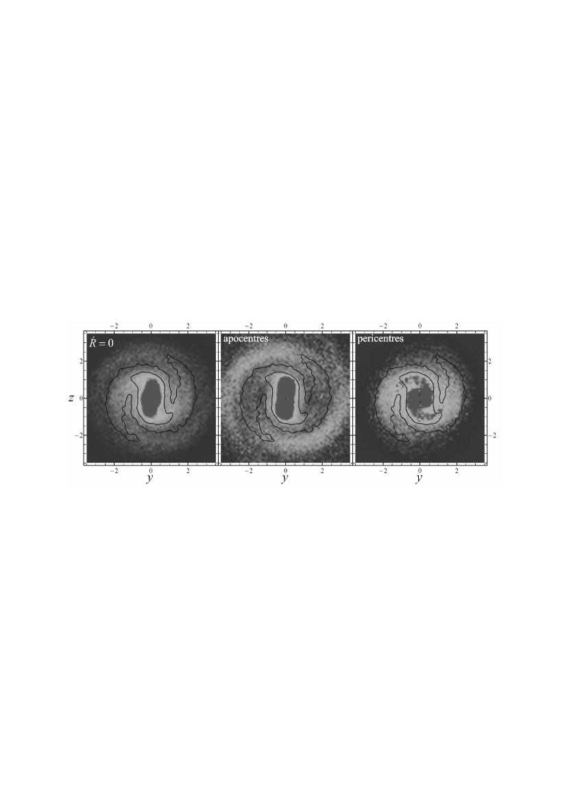
Figure 7: (a) The density distribution of the particles of Fig. 1 when integrated until their (cylindrical) radial velocities become zero ($\dot{R}=0$) for the first time, i.e. at the apocentres or the pericentres of their orbits. The density contours corresponding to the initial conditions of Fig. 1 are superimposed (black curves). (b) The density distribution of only the apocentres. The comparison with the density contours shows that the apocentres support the bar but not the extensive spiral arms. (c) The density distribution of only the pericentres. The comparison with the density contours shows that the pericentres support the spiral structure but not the bar.

In Fig. 5 we plot the effective potential of a 2D approximation of the system ($x=0$) along the $z$-axis ($V_{eff}(0,0,z)=V(0,0,z)-\frac{1}{2}\Omega_{p}^{2}z^{2}$, black dotted curve) and along the y-axis ($V_{eff}(0,y,0)=V(0,y,0)-\frac{1}{2}\Omega_{p}^{2}y^{2}$, black solid curve). The maximum of the black dotted curve corresponds to the Jacobi constant $E_{j}(L_{1})$ of the Lagrangian points $L_{1,2}$, while the maximum of the black solid curve corresponds to the Jacobi constant $E_{j}(L_{4})$ of the Lagrangian points $L_{4,5}$. For any Jacobi constant value below $E_{j}(L_{1})$, for example for $E_{j}=-1300000$ (dotted horizontal straight line), there is a forbidden region for the orbits (region between the two points of intersection with the effective potential curve). In this case, the phase space, as well as the configuration space, consists of two regions that do not communicate with each other (the one inside and the other outside corotation). By plotting the corresponding curve of the kinetic energy (dotted curve) and because of (Eq. 2), we see that for the region inside (outside) corotation the velocity minima correspond to the apocentres (pericentres) of the orbits. However, for $E_{j}$ values above $E_{j}(L_{4})$, for example for $E_{j}=-1050000$ (dashed horizontal straight line), the region inside corotation can communicate with the region outside corotation and the minimum velocity $v_{min}$ (minimum of the dashed curve) is found at the position of the maximum of the effective potential (i.e. the minimum difference of $E_{j}-V_{eff}$). In this case, the geometrical locus of the velocity minima on the configuration space is not directly related to the apocentres or the pericentres of the orbits.

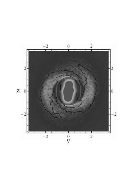
Figure 8: The density distribution of the particles of Fig. 1 (with $E_{j}<E_{j}(L_{4})$) at the positions corresponding to their local plane velocity minima ($v_{yz}=v_{min}$). We observe that this distribution fits well the morphology of the galaxy (black contour lines). In this figure we have omitted the particles with $E_{j}>E_{j}(L_{4})$ which are gathered along the geometrical locus of the maximum of the effective potential (gray elliptical curve).

Figure 6 presents the distribution of the velocities of the pericentres of the apocentres and of the velocity minima for three cases: (a) for orbits trapped outside corotation with $E_{j}<E_{j}(L_{1})$, (Fig. 6a), (b) for orbits inside corotation with $E_{j}<E_{j}(L_{1})$, (Fig. 6b) and (c) for orbits that can explore the whole permissible phase space inside and outside corotation with $E_{j}>E_{j}(L_{1})$, (Fig. 6c).

In Fig. 6a we observe that the pericentres of the orbits outside corotation have smaller velocities than the apocentres. Moreover the distribution of the velocity minima gives good agreement with the distribution of the velocities of the pericentres. At the same time, the distribution of the velocities of the apocentres almost coincide with the distribution of the velocity maxima (not plotted in the panel). Therefore, the particles outside corotation spend most of their time near the pericentres of their orbits which is consistent with the description of Fig. 5. On the other hand the opposite is true for particles inside corotation (Fig. 6b). The particles inside corotation have smaller velocities at their apocentres than at their pericentres. Moreover, the apocentric velocity distribution almost coincides with the distribution of the velocity minima. Here again the distribution of the velocity maxima (not plotted in the panel) almost coincides with the distribution of the velocities of the pericentres.

For the orbits having Jacobi constant above $E_{j}(L_{1})$ (Fig. 6c) even though there is not a clear breakoff of the distributions, the pericentres have statistically smaller velocities than the apocentres. Both pericentres and apocentres present a peak around the same value of velocity, which also coincides with the peak of the velocity minima distribution. The distribution of the apocentres, however, has a second important peak around a somewhat greater value of velocity.

In Fig. 7a we plot, in color scale, the density distribution of the particles of Fig. 1 taking each of them at a position corresponding to $\dot{r}=0$, i.e. at the apocentre or the pericentre of its orbit. The black curves correspond to the density contours of the space distribution shown in Fig. 1. Figure 7b presents, the density distribution of only the apocentres of the orbits. The corresponding density maxima inside corotation support the bar (since they correspond to loci of minimum velocities, see Fig. 6b) as well as a small extension of the bar to the inner parts of the spiral structure. However, the density maxima outside corotation, do not correspond to the density contours of the real spiral arms (black curves) but they extend far beyond. Figure 7c presents the density distribution of only the pericentres of the orbits. We see that these density maxima support a spiral structure very close to the real one, but a little more tight, and they do not support the bar.

Thus, we conclude that, in general, the apocentres of the orbits support the shape of the bar and the origins of the spirals near corotation, while the pericentres of the orbits better support the spiral structure near and outside corotation.

Figure 8 presents, in gray scale, the density distribution of the particles of Fig. 1 at positions corresponding to local minimum values of their rotation plane velocities ($v_{yz}=v_{min}$). The comparison with the density contours (black curves) of the initial conditions shows that the loci of the velocity minima reveal satisfactorily the features of the galaxy, i.e. the bar and the spiral arms. In this figure, however we have removed the overdensity of the particles along the theoretical locus of $v_{min}$ (gray elliptical curve) that represents the maximum of the effective potential ($V_{eff}$) for Jacobi constants above $E_{j}(L_{4})$, because it does not correspond to the distribution of the real particles.

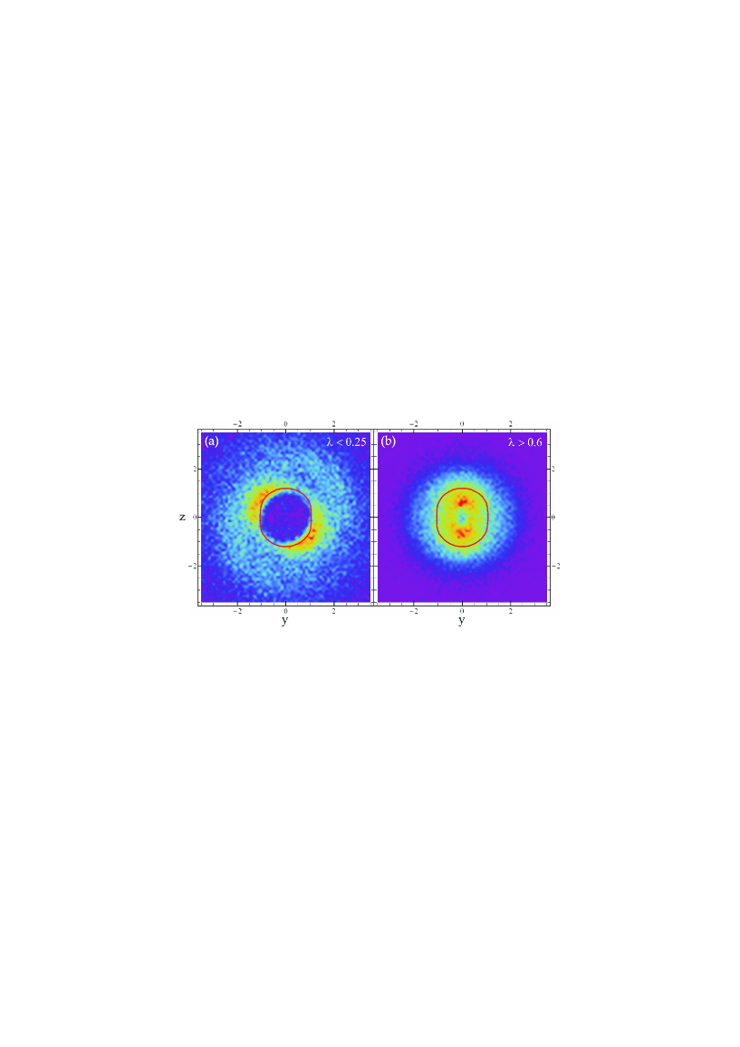
Figure 9: (a) The density distribution of the particles having $E_{j}>-977000>E_{j}(L_{4})$ and ratio $\lambda=\frac{<v_{\min}>}{<v_{yz}>}<0.25$ together with the locus corresponding to the effective potential maxima $V(eff)_{max}$ (red curve). The density maxima in this case are located near the curve of $V(eff)_{max}$ but along particular directions. (b) The same as in (a) but for particles having $\lambda=\frac{<v_{\min}>}{<v_{yz}>}>0.6$. The density maxima are located inside the curve of $V(eff)_{max}$ (see text for details).

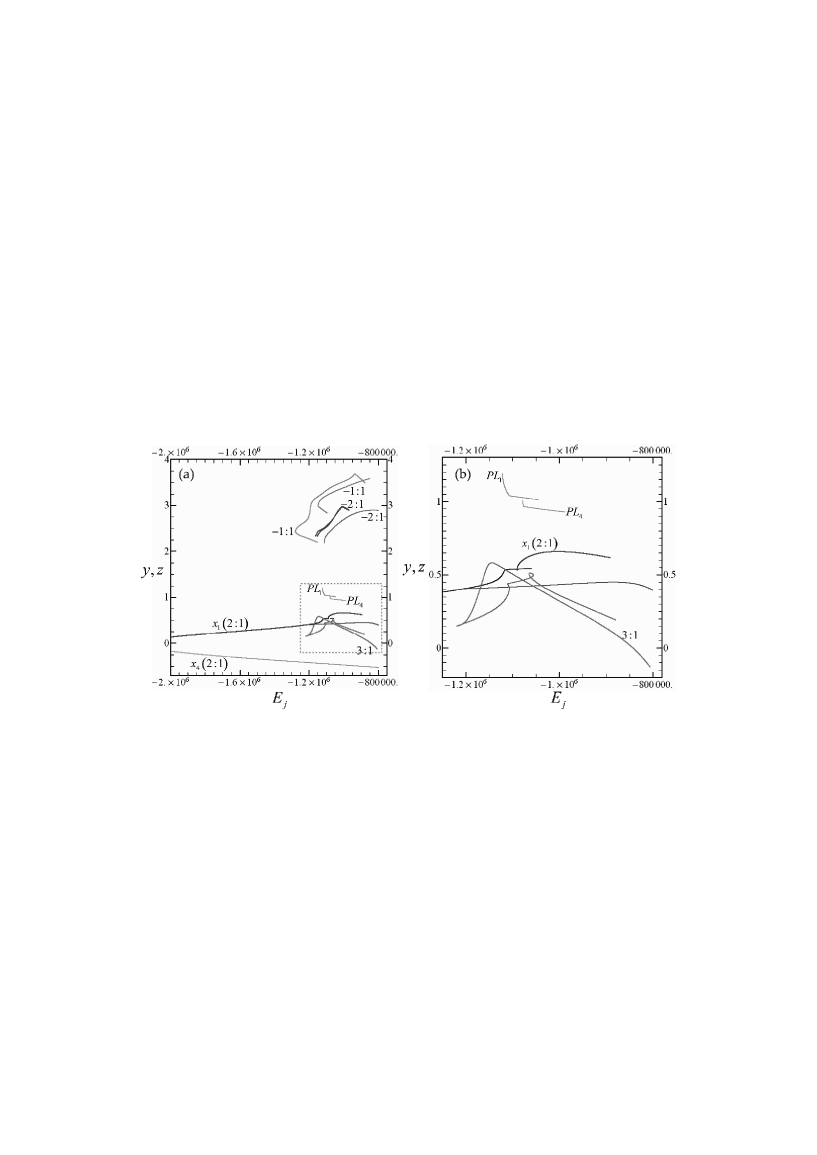
Figure 10: (a) The characteristics of the main 3D periodic orbits of the system. (b) A focusing in the inserted frame of (a).

Here we note that a density maximum in some area can be produced either by frequent (but not too short-lasting) transits or by long-lasting (but not too rare) transits of the particles through this area. For Jacobi constant values higher than $E_{j}(L_{4})$ the locus of the local velocity minima (red curve in Fig. 8) corresponds to velocity values that can be comparable to the mean velocity of the whole orbits. In Fig. 9 we have plotted the density distribution of the particles with Jacobi constant values $E_{j}>-977000>E_{j}(L_{4})$ corresponding to low and high values of the ratio $\lambda=<v_{\min}>/<v_{yz}>$ as indicated on the two panels of Fig. 9. We observe that the particles with low $\lambda$ values (Fig. 9a) form a ring-like density maximum area lying close to the locus of the maximum $V_{eff}$ (red curve). However the distribution is not uniform along the red curve, but it follows the distribution of the inner parts of the spiral arms. The maximum density area of the particles with high $\lambda$ values (Fig. 9b) is located inside the red curve corresponding to the velocity minima. In this case the density maxima are due to the more frequent transits of the orbits from this area.

4 Sticky Chaotic Orbits

In Figure 4 the frequency ratio $q$ of the chaotic population is plotted showing preferable concentrations around specific resonant periodic orbits. In order to study the behavior of sticky resonant orbits we find the characteristics of the most important periodic orbits in the 3D case. Figure 10 presents the characteristics of the main 3D periodic orbits, i.e. the $y$ ($z$ for the $PL_{4}$ family) component as a function of the Jacobi constant. We must point out that the periodic orbits $PL_{1}$ and $PL_{2}$ exist only above the value $E_{j}(L_{1})=-1120000$, while the periodic orbits $PL_{4}$ and $PL_{5}$ exist above the value $E_{j}(L_{4})=-1080000$. We will show below that all the important resonances, presented in the characteristic diagram (Fig. 10) and in the frequency analysis of the chaotic orbits (Fig. 4b), contribute to the formation of all the morphological features appearing in each Jacobi constant value.

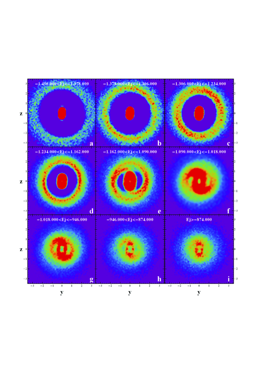
Figure 11: The density distribution on the $y-z$ plane of the particles belonging to nine different Jacobi constant bins. The corresponding values are marked on the top of each panel. The top left panel corresponds to the smallest values of Jacobi constants $E_{j}$ (close to the potential well) while the bottom right panel corresponds to the highest values of $E_{j}$’s. In this figure we reveal which structures are supported by the particles corresponding to the different Jacobi constant values.

Figure 11 presents, in color scale, the density distribution of particles on the rotation plane for nine different Jacobi constant levels. The top left panel corresponds to the lowest values of Jacobi constants $E_{j}$ (close to the potential well) while the bottom right panel corresponds to the highest values of $E_{j}$’s. The corresponding values of the Jacobi constant are marked on the top of each panel. Note that outside corotation (in energy levels with $E_{j}>E_{j}(L_{1})$) there exist practically only chaotic orbits (see Fig. 3). A general trend is that the space distribution of particles having lower values of Jacobi constants supports mostly the outer parts of the spiral arms as well as the shape of the bar, while particles having greater values of Jacobi constants support the inner parts of the spiral arms. This is obvious in Figs. 11 b-h, where we see a gradual shift of the maximum of the density distribution of particles outside corotation from the outer parts of the spiral arms to the inner parts and the innermost extensions of the bar (Figs. 11f,g). On the other hand there are levels of the Jacobi constant that do not support at all the spiral structure. This happens for the lowest values of the Jacobi constant near the potential well (Fig. 11a), where the distribution of particles outside corotation is quite uniform, and for the highest values of the Jacobi constant (Fig. 11i), where only chaotic orbits exist, which do not support the spiral structure but rather the outer parts of the bar.

Below we give some examples of the effect of stickiness (Contopoulos & Harsoula, 2008) of chaotic orbits around the unstable asymptotic manifolds of the unstable periodic orbits, in the phase space. We show that this stickiness supports the formation of the spiral structure, while the (slow) diffusion along the paths of the manifolds is responsible for the fadeout of this structure.

In the next subsections we give four examples of 3D chaotic orbits lying near and along some main unstable periodic orbits, having initial conditions inside corotation, near corotation and outside corotation.

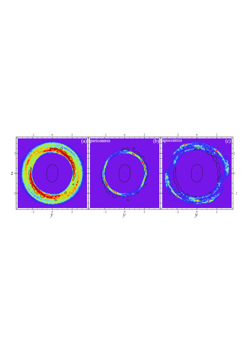
Figure 12: (a) The density distribution on the $y-z$ plane of 20000 3D orbits integrated for several $T_{hmct}$ having initial conditions close to and along the unstable periodic orbit $-1:1$ and Jacobi constant $E_{j}=-1252560$. Black curves indicate the high density contours of real particles corresponding to the same energy level. We note the coincidence of these density contours with the density maxima of the integrated orbits. (b) the density distribution of the pericentres superimposed with the high density contours of the corresponding energy level. (c) the same as in (b) but for the apocentres. We observe that the pericentres (apocentres) fit (do not fit) the density maxima of the real particles.

4.1 The -1:1 family

Figure 12 gives an example of the density distribution of orbits around an unstable periodic orbit of the $-1:1$ family with $E_{j}=-1252560$ (within the range of the top-right panel of Fig. 11) where the motion is limited outside corotation. We have taken 20000 initial conditions all along this 3D unstable periodic orbit (and its symmetric with respect to the origin), with small deviations from it, on the 6-dimensional space (${x,y,z,v_{x},v_{y},v_{z}}$). Then we integrated all these orbits for a time corresponding to many rotations of the bar. In Fig. 12a we plot the density distribution of these orbits on the rotation plane. In this figure we have considered a time interval within 5-6 bar rotations. In the same figure we have superimposed the high density contours of the corresponding Jacobi constant (black curves) and we see that the orbits close to the $-1:1$ periodic orbit reproduce well the density distribution giving the outer parts of the spiral structure. In Fig. 12b(12c) we plot the density distribution of the pericentres (apocentres) of the orbits of Fig. 12a together with the high density contours (black curves) corresponding to this $E_{j}$ value. On the one hand the pericentric density maxima seem to follow a part of the spiral structure but at a slightly smaller radius. On the other hand the apocentric distribution does not fit well the real density maxima. Finally we remark that the loci of the velocity minima practically coincide with the ones of the pericentres.

4.2 The 3:1 family

Figure 13 gives a similar information as Fig. 12, but for an unstable periodic orbit of the 3:1 family, which is located inside corotation for $E_{j}=-1090000$ (within the range of the middle-right panel of Fig. 11). This Jacobi constant value, is close to $E_{j}(L_{1})$, and the areas inside and outside corotation can communicate. We considered again 20000 initial conditions all along this 3D $(3:1)$ unstable periodic orbit (and its symmetric with respect to the origin), with small deviations from it, in the 6-dimensional space (${x,y,z,v_{x},v_{y},v_{z}}$). These orbits follow, in the phase space, the unstable directions of the asymptotic manifolds originating from the periodic orbit. For a short time (the shortness depends on how large is the initial divergence from the periodic orbit) these orbits stay very close to the periodic orbit, but later they start deviating considerably from it. In Fig. 13a we see the density distribution (in color scale) of these orbits after within a time interval of 3-4 bar rotations. The black curves indicate the high density contours of the real particles for the same Jacobi constant value. It is evident that these two distributions fit one another very well. A similar behavior has been found by Patsis (2006) for chaotic orbits near the 4:1 resonance. This type of orbits was considered responsible for the inner parts of the spiral arms in an analytical model representing the spiral galaxy NGC 4314.

In Fig. 13b we have plotted the positions of all the orbits for the time interval of Fig. 13a. The color of each point shows the corresponding velocity value on the rotation plane. The color scale is the same as for the densities (see Fig. 1) which means that blue color corresponds to the minima and red color to the maxima of the velocity values. We observe that the density maxima are well correlated with the areas of small velocity values (dark to light blue colors in Fig. 13b). Figures 13c,d are similar to Figs. 12b,c. We observe that the pericentres of the orbits (Fig. 13c) form a slightly more closed spiral structure than that of the real particles (black density contours). On the other hand the apocentres of the orbits (Fig. 13d) fit well only the density contours of the bar and the innermost parts of the spiral structure that originate from the end of the bar. In Fig. 13e we plot the density distribution of the loci of the local velocity minima. We notice that this distribution matches better the distribution of the apocentres in what concerns the bar and the distribution of the pericentres in what concerns the spiral structure.

4.3 The 2:1 ($x_{1}$) family

The 2:1 (or $x_{1}$ after the nomenclature of Contopoulos & Papayannopoulos, 1980) family is generally considered responsible for the formation and the robustness of the bar. This is due to its morphology, together with the fact that this family is usually stable for low values of the Jacobi constant. According to this point of view the bar should end not beyond the point where the $x_{1}$ family turns from stable to unstable. Here we point out the usefulness of the unstable part of this family which supports the spiral structure. Figure 14a,b is similar to Fig. 13a,b but for the $x_{1}$ family and for the same Jacobi constant value. We observe that the density of the orbits starting close to the $x_{1}$ periodic orbit is similar to the density of the orbits with initial conditions near the 3:1 periodic orbit. Their density maxima support the morphological structures (bar and spiral) of the real particles for the same Jacobi constant value (Fig. 14a). These maxima lie near the areas corresponding to low values of plane velocities $v_{yz}$ (Fig. 14b).

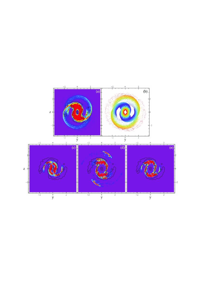
Figure 13: (a) The density distribution on the $y-z$ plane of 20000 3D orbits having initial conditions close to and along the unstable periodic orbit 3:1 (and its symmetric with respect to the origin) at $E_{j}=-1090000$. The plotted distribution corresponds to a time interval within 3-4 bar rotations. Black curves denote density contours of the real particles corresponding to the same Jacobi constant value. (b) The positions of all the orbits at the snapshot shown in (a). The color of each point indicates the corresponding velocity value on the rotation plane. The color scale is the same as for the densities (see Fig. 1). (c) The density distribution of the pericentres superimposed with the density contours of the corresponding Jacobi constant value. (d) The same as in (c) but for the apocentres. (e) The same as in (c) but for the local velocity minima $v_{min}$.

4.4 The $PL_{1,2}$ families

Figure 15 is similar to Fig. 14 but for the unstable periodic orbits $PL_{1,2}$ which are located near corotation and for the same Jacobi constant value. In this case we establish the same behavior (as for the cases 3:1 and $x_{1}$) for the orbits initiating close to the symmetric periodic orbits $PL_{1,2}$. The orbits starting near the periodic orbits 3:1, 2:1, $PL_{1,2}$ follow the unstable directions of the asymptotic manifolds originating from these periodic orbits. For the same Jacobi constant value these manifolds cannot intersect each other, and this means that these manifolds are parallel in the phase space. Thus, the orbits along the unstable directions of the various manifolds follow parallel paths and present a similar behavior in the configuration space. The major difference between the different sets of orbits starting near the different unstable periodic orbits (3:1, 2:1, $PL_{1,2}$) is the diffusion rate (see section 5), which increases towards higher resonance orders $(2:1\rightarrow 3:1\rightarrow\infty:1\equiv PL_{1,2})$.

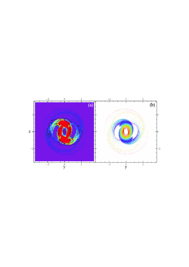
Figure 14: Similar to Figs. 13a,b but for the unstable periodic orbit 2:1 $(x_{1})$ and for the same Jacobi constant value.

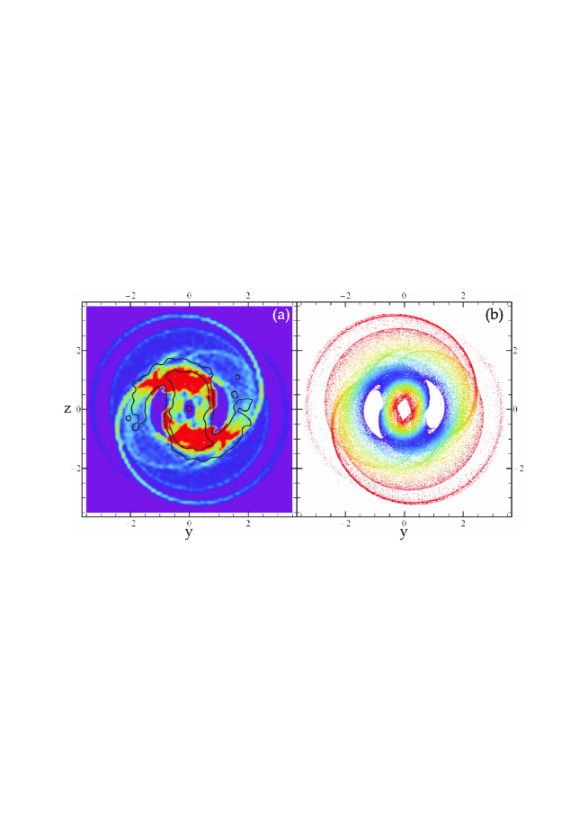
Figure 15: Similar to Figs. 13a,b but for the unstable periodic orbits $PL_{1,2}$ and for the same Jacobi constant value.

4.5 Other families

All the other families of periodic orbits have similar behavior to those studied in Figs.12-15. Thus, the behavior of the orbits with $-1300000\lesssim E_{j}<E_{L_{1}}$ lying outside corotation (e.g. $-2:1$) resembles that of the $-1:1$ family (Fig. 12) supporting the outer parts of the spiral structure. Families lying inside corotation with $E_{j}>E_{L_{1}}$ (e.g. 4:1, $PL_{4,5}$) behave similarly to the families 2:1, 3:1, $PL_{1,2}$ (Figs. 13-15) and support the bar and the inner parts of the spiral arms connected to the bar. Note that there are chaotic orbits associated with the 2:1, 3:1 and 4:1 families, located inside corotation for $E_{j}<E_{L_{1}}$ that support the envelope of the bar (Harsoula & Kalapotharakos, 2009). Some of the characteristics of these families are plotted in Fig. 10. Moreover, in Fig. 4b we see many real particles that stick around various resonances both inside and outside corotation (see the various spikes corresponding to different resonances).

4.6 Reconstruction of the galaxy by the superposition of the main families

The chaotic orbits close to the unstable periodic orbits corresponding to different Jacobi constant values may form different density distributions. However, the orbits at every Jacobi constant support the density distribution of the real particles at the same value of the Jacobi constant. Here we demonstrate what is the contribution of a family, all along its characteristic, to the global morphology of the galaxy. This is done in Fig. 16 for the 3:1 family. In Fig. 16a we plot 100 periodic orbits (black points) of the 3:1 family equally sampled along its whole characteristic together with the density contours of the galaxy (black lines). These orbits are located inside corotation. In Fig. 16b we plot the density distribution of 20000 orbits having initial conditions close and along the periodic orbits of Fig. 16a integrated for 3-4 bar rotations. Although the initial conditions are all inside corotation supporting the bar shape, after a short transient period of stickiness along the periodic orbits they are diffused outside corotation and form a spiral structure which is slightly more closed than that of the galaxy (Fig. 16b).

Figure 17 is similar to Fig. 16 but for the 2:1 (or $x1$) family. Note that the superposition of the periodic orbits do not cover the inner parts of the bar since we have chosen only the unstable periodic orbits along the characteristic of the 2:1 family. In Fig. 17b we see that the orbits starting close to the periodic orbits of Fig. 17a form a spiral structure fitting well the inner part of the spiral structure of the galaxy (black curves).

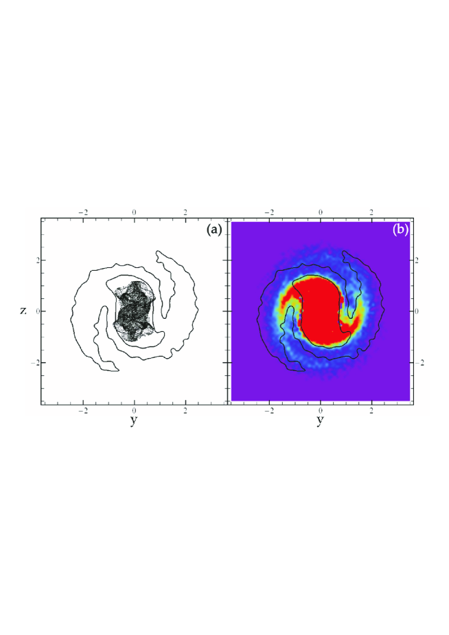
Figure 16: (a) The projection on the $y-z$ plane of 100 periodic orbits (black points) of the 3:1 family equally sampled along its whole characteristic together with the density contours of the galaxy (black lines). (b) the density distribution on the $y-z$ plane of 20000 orbits with initial conditions close and along the periodic orbits shown in (a) after integration for 3-4 bar rotations.

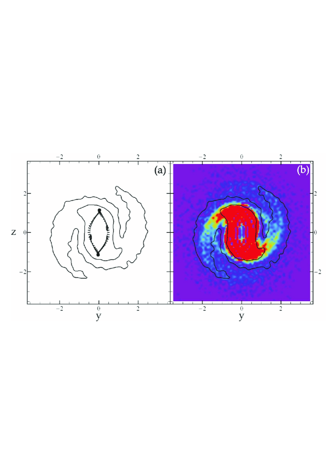
Figure 17: Similar to Fig. 16 but for the unstable part of the 2:1 family.

Finally, Fig. 18 provides the same information as Figs. 16,17 but for the $-1:1$ family. It is evident that the density maxima of the density distribution of these orbits support the outer parts of the spiral structure of the galaxy. The same picture is also true for the other families outside corotation that have $q<0$ (e.g. the -2:1 family).

In Fig. 19 we plot the superimposed density distributions of the orbits shown in Figs. 16b,17b,18b (color scale) together with the high density contours of the galaxy (black curves). We observe that the galaxy is well reconstructed by this set of orbits. This figure clearly underlines the importance of the unstable periodic orbits and of the chaotic orbits associated with them in forming the spiral structure.

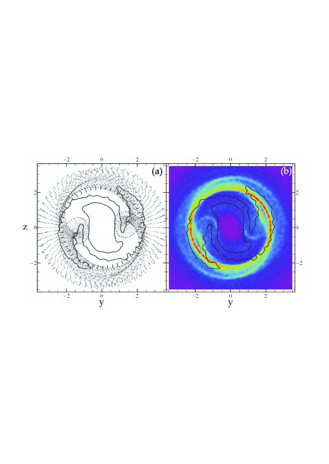
Figure 18: Similar to Fig. 16 but for the $-1:1$ family.

4.7 2D Asymptotic Orbits

The main results of the above study, for the 3D orbits along specific important resonances of the system can be also acquired if we study the space distribution of the pericentres or apocentres of the asymptotic orbits in a 2D approximation of the system ($x=0,\dot{x}=0$ in Eq. 2). Namely, if we consider 2D unstable periodic orbits (the most important for every energy level) and take initial conditions along their unstable asymptotic curves, the integration of these asymptotic orbits can also reveal the morphological features of every energy level.

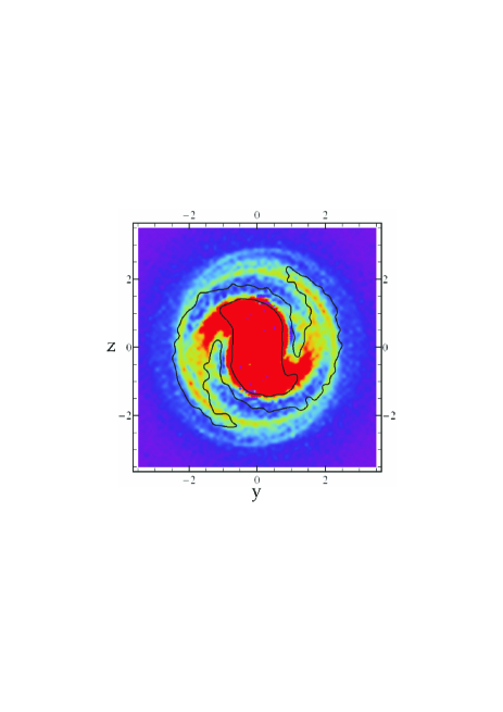
Figure 19: The superposition of all the distributions shown in Figs. 16b,17b,18b superimposed with the density contours of the galaxy (black curves). All the main morphological features of the galaxy are reconstructed by the superposition of these orbits.

In Fig. 20a, 20b we give an example of the projection on the configuration space of the apocentric and pericentric intersections (black points), respectively, of the 2D manifold of the $-2:1$ unstable periodic orbit corresponding to $E_{j}=-1135000<E_{j}(L_{1})$ where the areas inside and outside corotation cannot communicate. Note that the phase space in the area outside corotation, in the 2D approximation of the system, presents no tori or cantori with small holes, but only a chaotic sea with escapes to infinity. In each panel of Fig. 20 we have superimposed the density distribution (in color scale) of the real particles at the same Jacobi constant value. We observe that the apocentres do not coincide with the maxima of the density while the pericentres trace well the areas of the density maxima, but for slightly smaller radii. This is compatible to the information provided by Fig. 12 according to which for Jacobi constant values below $E_{j}(L_{1})$ and outside corotation the pericentres reveal the density maxima since they lie near low values of the plane velocity.

Figure 21 is similar to Fig. 20 but for a different Jacobi constant $E_{j}$=-1120000, which is just above $E_{j}(L_{1})$, and therefore the area inside corotation has just communicated with the area outside corotation. In this energy level and in the 2D approximation there exist unstable periodic orbits of the $PL_{1}$, $PL_{2}$ and $-1:1$ families. In Fig. 21a,b we plot the apocentres and the pericentres, respectively, of all the asymptotic orbits (having initial conditions on the unstable asymptotic curves) of all the periodic orbits mentioned above, superimposed on the density distribution of the real particles in the specific Jacobi constant value. In this case we see that the pericentres together with some parts of the apocentres (mostly of the $PL_{1}$, $PL_{2}$ families) trace well the density maxima of the density distribution. This is compatible to the information provided by Fig. 13 according to which the pericentres and the apocentres for Jacobi constant values above $E_{j}(L_{1})$ reveal the density maxima when they lie near low values of the plane velocity.

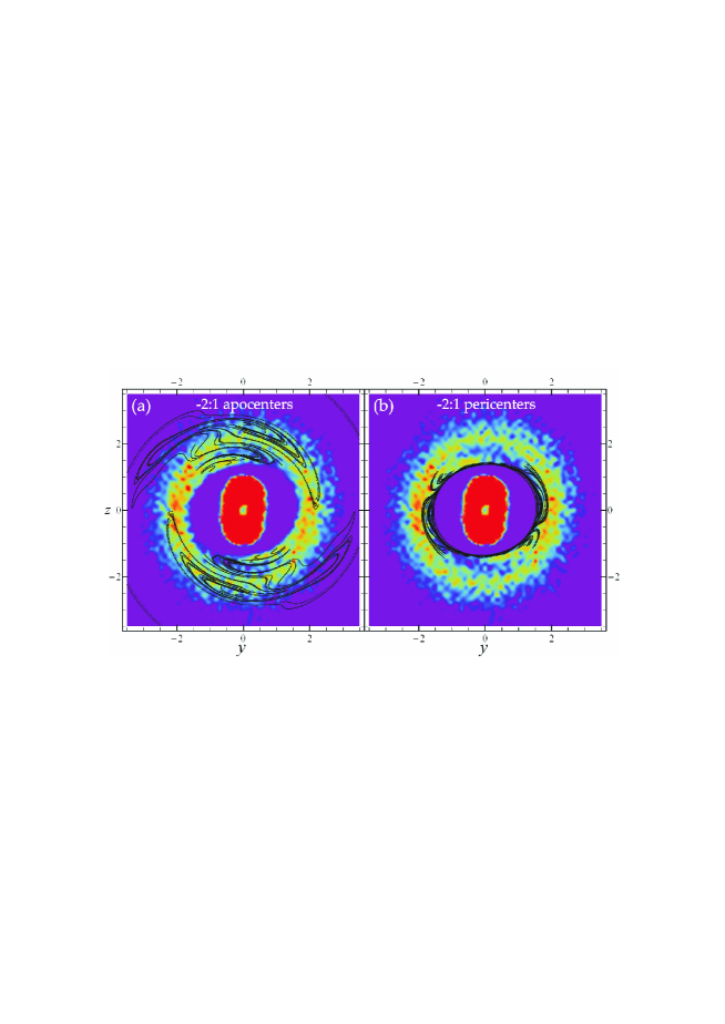
Figure 20: (a), (b) The projection on the configuration space of the apocentric and pericentric intersections (black points), respectively, of the 2D manifold of the $-2:1$ unstable periodic orbit corresponding to $E_{j}=-1135000<E_{j}(L_{1})$ where the areas inside and outside corotation cannot communicate superimposed on the density distribution of the real particles of this Jacobi constant value.

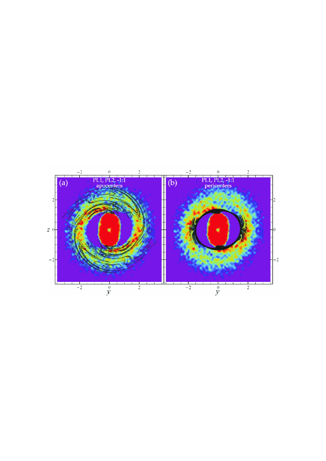
Figure 21: Similar to Fig. 20 but for the manifolds of the $PL_{1,2}$ and $-1:1$ families and for $E_{j}=-1120000$ just above $E_{j}(L_{1})$.

5 Rays, Bell-type curves and Escaping orbits

The stickiness effect along the asymptotic manifolds of the unstable periodic orbits can last for a number of dynamical times reinforcing the spiral structure, as it has been described in the previous sections, but then the chaotic orbits can escape to very large distances and finally they may escape to infinity. This diffusion is relatively slow and its time scale can be compared to the age of the Universe. In this section we study the way these chaotic orbits escape to infinity.

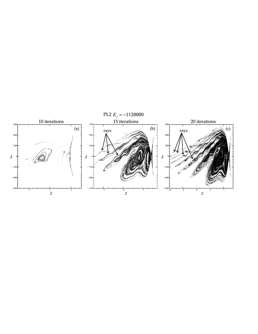
Figure 22: The asymptotic curves of the unstable periodic orbit $PL_{2}$ in the phase space ($z,\dot{z}$) (for $y=0$ and $\dot{y}>0$) for the 2D approximation of our model and for $E_{j}=-1120000$ close to $E_{j}(L_{1})$ after (a) 10 iterations (b) 15 iterations and (c) 20 iterations of a small initial segment along the unstable directions of the manifold.

Figure 22 presents the unstable asymptotic curve of the $PL_{2}$ orbit on a Poincar$\acute{e}$ surface of section $z,\dot{z}$ for $y=0$ and $\dot{y}>0$ of the 2D approximation of the system and a Jacobi constant close to $E_{j}(L_{1})$. We have taken a small initial segment of 50000 points and of length $10^{-6}$ from the unstable periodic orbit and along the direction of the unstable asymptotic curve, and we have integrated all these points for 10 iterations (Fig. 22a) 15 iterations (Fig. 22b) and 20 iterations (Fig. 22c). We observe the formation of characteristic rays along the asymptotic curves when integrated for a long time.

In Fig. 23 we see the picture of the same Poincar$\acute{e}$ surface of section after the integration of 100 initial conditions of test particles for 200 iterations in the 2D approximation of the system (black points). These points are concentrated close to the unstable asymptotic curves of the families $PL_{1}$, $PL_{2}$. In Fig. 23 we also plot the curves corresponding to zero inertial energy $E=0$ (thick black curves). The analytic relation $\dot{z}=f(z)$ (for $y=0$) describing these curves is found as follows: By subtracting Eqs. 2 and 6 for $E=0$ and $\dot{x}=x=y=0$ we find

$$\Omega_{p}\dot{y}z+\Omega^{2}_{p}z^{2}=-E_{j}$$ (8)

where

$$\dot{y}=\pm\sqrt{2E_{j}+\Omega^{2}_{p}z^{2}-2V(0,0,z)-\dot{z}^{2}}$$ (9)

Hence

$$\dot{z}^{2}=-2V(0,0,z)-\frac{E^{2}_{j}}{\Omega^{2}_{p}z^{2}}$$ (10)

This last equation gives two symmetric curves, one with $\dot{z}<0$ and the other with $\dot{z}>0$, shown by thick black curves in Fig. 23. Orbits starting below the lower thick black curve escape to infinity without intersecting the $E=0$ curve. An example is given by the blue dots, numbered 1,2,3,…, which correspond to the successive iterations of an initial condition near the point $1$, having $E>0$. These iterations are located along rays. The corresponding orbit escapes from the galaxy following a spiral path, in the rotating configuration space (see inserted orbit in Fig. 23). On the other hand, if an initial condition has $E<0$, then the successive iterations (red dots) lie on rays again, but between the two $E=0$ curves, and at the same time they form “bell-type” curves (Contopoulos and Patsis 2006). Different bell-type curves correspond to different values of the energy $E$. The value of $E$ along an orbit remains roughly constant far from the galaxy (left part of Fig. 23) forming a bell-type curve, but it changes abruptly whenever the orbit comes close to the main body of the galaxy (small absolute values of $z$) and then it follows a new bell-type curve. The changes of $E$ are irregular, due to the chaotic character of the orbit. After several changes of its value, $E$ becomes positive, and then the orbit escapes to infinity following a spiral-like path. Note that this path corresponds to an open hyperbolic curve in an inertial frame of reference.

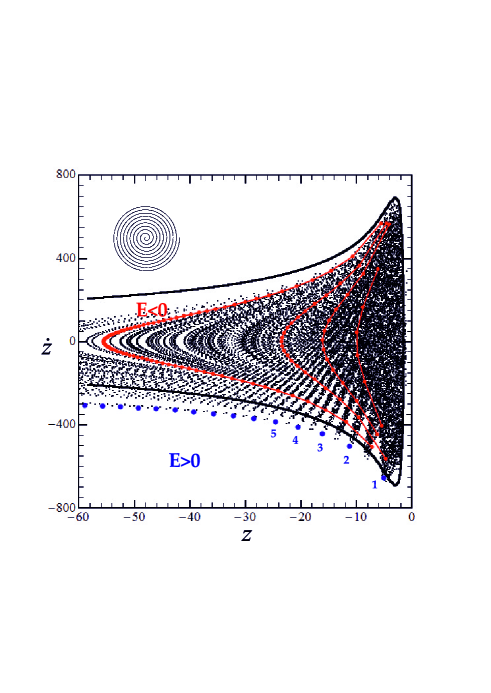
Figure 23: The phase space $z$, $\dot{z}$ (for $y=0$ and $\dot{y}>0$) of a 2-D approximation of our model for a Jacobi constant $E_{j}=-1120000>E_{j}(L_{1})$, where the area inside corotation can communicate with the area outside corotation. The thick black curves correspond to zero inertial energy. An initial condition near the point $1$ and inertial energy $E>0$ has successive iterations (blue dots) along rays and escape to infinity following a spiral like orbit (inserted orbit). On the other hand if we take initial conditions having $E<0$ the successive iterations (red dots) lie along rays and along bell type curves at the same time.

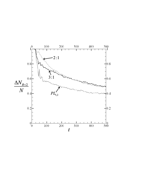
Figure 24: The percentage of the orbits starting close to the 3:1, 2:1, $PL_{1,2}$ unstable periodic orbits (see Figs. 13-15) that stay located inside $R=2r_{hm}$ as a function of time in $T_{hmct}$.

Finally, Fig. 24 presents the fraction of the particles starting close to the 3:1, 2:1, $PL_{1,2}$ periodic orbits (see Fig. 13-15) that stay located inside a radius of $2r_{hm}$ as a function of time in $T_{hmct}$. This figure testifies the phenomenon of stickiness along the manifolds originating from the unstable periodic orbits and gives a measure of the chaotic diffusion of the system. We observe two different rates of diffusion: (a) the first one lasts for 50 to 100 $T_{hmct}$ where about the 20%, 25% and 45% of the orbits around the 2:1, 3:1 and $PL_{1,2}$ periodic orbits respectively have been diffused outwards and (b) a quite slower diffusion starting after $\approx 100T_{hmct}$. In general, orbits with initial conditions closer to lower order $n$ of resonance $n:1$ present a slower diffusion rate. During the first diffusion period, the spiral structure is viable, because the flow of chaotic material coming from inside corotation stay confined close and along the asymptotic manifolds of the unstable periodic orbits and support the spiral structure of the galaxy. This time period corresponds to about 10 rotations of the bar. After that and during the second period of slow diffusion where chaotic orbits move outwards, spiral structure is not clearly observed in the system.

6 CONCLUSIONS

In this paper we study the main factors that affect the formation and the longevity of the stellar spiral arms of barred spiral galaxies. We examine the role of the apocentres, of the pericentres and of the velocity minima as regards the morphological features of a galaxy. We emphasize the role of the asymptotic orbits, emanating from the unstable periodic orbits, in forming different segments of the spiral arms corresponding to different values of the Jacobi constant inside and outside corotation. We show that there is stickiness along these asymptotic orbits which affects the longevity of the spiral arms, which finally fade away, but after more than 10 bar rotations. Below we present and discuss our main results.

(a)

An objective way to find the maxima of density is by finding the loci of the velocity minima on the rotation plane, since the particles spend most of their time there. These loci are:

1. The apocentres for the particles with Jacobi constants below $E_{L_{1}}$ that are allowed to move only inside corotation. These apocentres, of regular or chaotic orbits, support the shape of the bar. The regular orbits form the main body of the bar, while the chaotic orbits form an envelope of the bar.

2. The pericentres for the particles with Jacobi constants below $E_{L_{1}}$ that are allowed to move only outside corotation. These pericentres support the outer parts of the spiral structure of the galaxy.

3. An elliptical locus corresponding to the local maximum of the effective potential $V_{eff}$ for the particles with Jacobi constant $E_{j}>E_{j}(L_{4})$ that are allowed to move both inside and outside corotation. This locus is only partly realized in the distribution of the real $N$-body particles, because an important percentage of particles with $E_{j}>E_{j}(L_{4})$ have minimum velocities $v_{min}$ that do not differ significantly from the mean velocity $<v_{yz}>$ all along their orbits. Therefore, this locus is not reflected in the global configuration of the particles although it is reflected in the sub-population corresponding to low $v_{min}$ values compared to $<v_{yz}>$.

For Jacobi constants $E_{j}(L_{4})>E_{j}>E_{j}(L_{1})$ some of the loci of pericentres and apocentres that are close to low values of the velocity are correlated to the inner parts of the spiral structure.

(b)

For each value of the Jacobi constant there is a set of stable and unstable periodic orbits. It is well known that the domain of phase space associated with the stable periodic orbits supports features similar to the morphologies of these orbits.

On the other hand in the present study we emphasize the role of the unstable periodic orbits and the manifolds emanating from them. Although the unstable periodic orbits themselves do not support the spiral structure, the asymptotic orbits that start near the unstable periodic orbits support the spiral structure. As long as there is a particle population near the unstable periodic orbits of the main families of orbits (e.g. -1:1, -2:1, $PL_{1}$, $PL_{2}$, $PL_{4}$, $PL_{5}$, 4:1, 3:1 and 2:1) the spiral structure remains clearly visible. We show that the superposition of orbits with initial conditions close to the periodic orbits of only three main families (-1:1, 2:1, 3:1) all along their characteristics are able to reconstruct all the main morphological features of the galaxy.

(c)

For Jacobi constants above $E_{j}(L_{1})$ chaotic diffusion leads to escapes. The diffusion is fast (for all the families) for a time interval lasting for about 10 rotations. Afterwards, the diffusion rate slows down but the spiral structure is marginally discernible. For the families inside and close to corotation (e.g. 2:1, 3:1, 4:1, $PL_{1}$, $PL_{2}$) the diffusion rate is smaller for orbits closer to the center. On the other hand, chaotic orbits having initial conditions outside corotation present stickiness at the resonances $-1:1$ and $-2:1$ and support the outer parts of the spiral structure.

The stickiness of the chaotic orbits along the unstable asymptotic curves, is called “stickiness in chaos” (Contopoulos & Harsoula, 2008), as it is not due to islands of stability or cantori. The shape of these asymptotic curves in the phase space (”rays”) corresponds to the shape of the spiral structure in the configuration space.

In our model, the phase space outside corotation is not bounded. Therefore, chaotic orbits above and outside corotation will finally acquire positive energy and escape from the system, along spiral orbits (in the rotating frame of reference). The successive iterations of chaotic orbits with negative inertial energy, in the phase space, lie on bell-type curves, each corresponding to the same energy. However, the energy changes when a star approaches the main body of the galaxy. Once a chaotic orbit acquires positive energy it has successive iterations that lie on rays that extend to infinity. This escape will happen, in general, after times considerably longer than the age of the Universe.

Finally, we note that our model is an adiabatic approximation of a real $N$-body system. Such a study is capable of providing the main trends about the dynamical mechanisms of the formation and the longevity of the various structures. However, the dynamical behavior of the real system is definitely more complicated since it shows an evolution (decrease) of the pattern speed (although this decrease is rather small). Another issue has to do with the evolution of the density and consequently of the potential. In our “frozen” model the amplitude of the spiral perturbation in the density decreases with time. The change of these two parameters affects the phase space structure. This implies a different network of unstable periodic orbits and also different asymptotic orbits with different stickiness around them. An extended study of the real evolving system requires the use of dynamical methods that take into account the evolution of both the pattern speed and the potential. We have proceeded in this direction and we will present our results in a forthcoming paper.

References

- Athanassoula et al. (2009a) Athanassoula, E.M., Romero-Gomez, M., Masdemont, J.J.,2009a, MNRAS, 394, 67.
- Athanassoula et al. (2009b) Athanassoula E., Romero-Gomez M., Bosma A., Masdemont J.J., 2009b, MNRAS, 400, 1706.
- Binney & Tremaine (1987) Binney J., Tremaine S., 1987, ”Galactic Dynamics”, Princeton University Press.
- Contopoulos (1975) Contopoulos, G., 1975, ApJ, 201, 566.
- Contopoulos & Papayannopoulos (1980) Contopoulos G., Papayannopoulos T., 1980, A&A, 92, 33.
- Contopoulos (1981) Contopoulos, G., 1981, A&A, 102, 265.
- Contopoulos & Grosbol (1989) Contopoulos, G., Grosbol, P., 1989, A&A, 1, 261.
- Contopoulos & Patsis (2006) Contopoulos, G., Patsis, P.A., 2006, MNRAS, 369, 1039.
- Contopoulos & Harsoula (2008) Contopoulos, G. Harsoula, M., 2008, Int. J. Bif. Chaos 18, 2929.
- de Zeeuw (1985) de Zeeuw, T., 1985, MNRAS, 216, 273.
- Fathi et al. (2009) Fathi, K., Beckman, J. E., Pinol-Ferrer, N., Hernandez, O., Martinez-Valpuesta, I., Carignan, C., 2009, ApJ, 704, 1657.
- Grosbol et al. (2004) Grosbol,P., Patsis, P.A., Pompei, E., 2004, A&A, 423, 849.
- Harsoula & Kalapotharakos (2009) Harsoula, M. Kalapotharakos, C., 2009, MNRAS, 394, 1605.
- Kalnajs (1971) Kalnajs A.J., 1971, ApJ, 166, 275.
- Kaufmann & Contopoulos (1996) Kaufmann D.E., Contopoulos G., 1996, A&A, 309, 381.
- Lin & Shu (1964) Lin, C. C. and Shu, F. H., 1964, Astrophys. J. 140, 646.
- Lynden-Bell & Kalnajs (1972) Lynden-Bell D., Kalnajs A.J., 1972, MNRAS, 157, 1.
- Merritt (1996) Merritt, D., 1996, Science, 271, 337.
- Patsis et al. (2002) Patsis P.A., Skokos Ch., Athanassoula E., 2002, MNRAS, 337, 578.
- Patsis (2006) Patsis, P.A., 2006, MNRAS, 369, L56.
- Romero-Gomez et al. (2006) Romero-Gomez, M.,Masdemont, J.J., Athanassoula, E.M., Garcia-Gomez, C. 2006, A&A, 453, 39.
- Romero-Gomez et al. (2007) Romero-Gomez, M., Athanassoula, E.M.,Masdemont, J.J., Garcia-Gomez, C., 2007, A&A, 472,63.
- Shen & Sellwood (2004) Shen, J., Sellwood, J.A., 2004, 604, 614.
- Sparke & Sellwood (1987) Sparke L., Sellwood J.A., 1987, MNRAS, 225, 653.
- (25) Toomre, A., 1977, Ann. Rev. Astron. Astrophys., 15, 437.
- (26) Tsoutsis P., Efthymiopoulos C., Voglis N., 2008, MNRAS, 387, 1264.
- Voglis et al. (2006a) Voglis N., Tsoutsis P., Efthymiopoulos C., 2006a, MNRAS, 373, 280.
- Voglis et al. (2006b) Voglis N., Stavropoulos I., Kalapotharakos C., 2006b, MNRAS, 372, 901.